A Fast Distributed Approximation Algorithm for Minimum Spanning Trees Maleq Khan and Gopal Pandurangan Department of Computer Science, Purdue University, West Lafayette, IN 47907, USA {mmkhan, gopal}@cs.purdue.edu
Abstract. We present a distributed algorithm that constructs an O(log n)-approximate minimum spanning ˜ tree (MST) in any arbitrary network. This algorithm runs in time O(D(G) + L(G, w)) where L(G, w) is a parameter called the local shortest path diameter and D(G) is the (unweighted) diameter of the graph. Our algorithm is existentially optimal (up to polylogarithmic factors), i.e., there exists graphs which need Ω(D(G) + L(G, w)) time to compute an H-approximation to the MST for any H ∈ [1, Θ(log n)]. Our result also shows that there can be a significant time gap between exact and approximate MST computation: there exists graphs in which the running time of our approximation algorithm is exponentially faster than the time-optimal distributed algorithm that computes the MST. Finally, we show that our algorithm can be used to find an approximate MST in wireless networks and in random weighted networks in almost optimal ˜ O(D(G)) time.
Keywords: Minimum Spanning Tree, Distributed Approximation Algorithm, Randomized Algorithm.
1 1.1
Introduction Background and Previous Work
The distributed minimum spanning tree (MST) problem is one of the most important problems in the area of distributed computing. There has been a long line of research to develop efficient distributed algorithms for the MST problem starting with the seminal paper of Gallager et al [1] that constructs the MST in O(n log n) time and O(|E| + n log n) messages. The communication (message) complexity of the Gallager et al. algorithm is optimal, but its time complexity is not. Hence further research concentrated on improving the time complexity. The time complexity was first improved to O(n log log n) by Chin and Ting [2], further improved to O(n log∗ n) by Gafni [3], and then improved to existentially optimal running time of O(n) by Awerbuch [4]. The O(n) bound is existentially optimal in the sense that there exists graphs where no distributed MST algorithm can do better than Ω(n) time. This was the
2
state of the art till the mid-nineties when Garay, Kutten, and Peleg [5] raised the question of identifying graph parameters that can better capture the complexity (motivated by “universal” complexity) of distributed MST computation. For many existing networks G, their diameter D(G) (or D for short) is significantly smaller than the number of vertices n and therefore is a good candidate to design protocols whose running time is bounded in terms of D(G) rather than n. Garay, Kutten, and Peleg [5] gave the first such distributed algorithm for the MST problem with running time O(D(G) + n0.61 ), which was later improved by Kutten and Peleg [6] to O(D(G) +
√
n log∗ n). Elkin [7] refined this result further and argued that a pa-
rameter called “MST-radius” captures the complexity of distributed MST algorithms better. √ ˜ He devised a distributed protocol that constructs the MST in O(µ(G, w) + n) time, where µ(G, w) is the “MST-radius” of the graph [7] (is a function of the graph topology as well as the edge weights). The ratio between diameter and MST-radius can be as large as Θ(n), and consequently, on some inputs, this protocol is faster than the protocol of [6] by a factor of √ Ω( n). However, a drawback of this protocol (unlike the previous MST protocols [6, 5, 2, 3, 1]) is that it cannot detect the termination of the algorithm in this much time (unless µ(G, w) is given as part of the input). Finally, we note that the time-efficient algorithms of [6, 7, 5] are not message-optimal (i.e., they take asymptotically much more than O(|E| + n log n) messages, e.g., the protocol of [6] takes O(|E| + n1.5 ) messages).
The lack of progress in improving the result of [6], and in particular breaking the
√
n bar-
rier, led to work on lower bounds for the distributed MST problem. Peleg and Rabinovich [8] ˜ √n) time is required for constructing an MST even on graphs of small diameshowed that Ω( ter and showed that this result establishes the asymptotic near-tight (existential) optimality of the protocol of [6].
3
While the previous distributed protocols deal with computing the exact MST, the next important question addressed in the literature concerns the study of distributed approximation of the MST, i.e., constructing a spanning tree whose total weight is near-minimum. From a prac˜ √n) time, it is worth tical perspective, given that MST construction can take as much as Ω( investigating whether one can design distributed algorithms that run faster and output a nearminimum spanning tree. Peleg and Rabinovich [8] was one of the first to raise the question of devising faster algorithms that construct an approximation to the MST and left it open for further study. To quote their paper: “To the best of our knowledge, nothing nontrivial is known about this problem...”. Since then, the most important result known till date is the hardness results shown by Elkin [9]. This result showed that approximating the MST problem on graphs of small diameter (e.g., O(log n)) within a ratio H requires essentially Ω(
p
n/HB) time (assum-
ing B bits can be sent through each edge in one round), i.e., this gives a time-approximation p trade-off for the distributed MST problem: T 2 H = Ω( n/B). However, not much progress has been made on designing time-efficient distributed approximation algorithms for the MST problem. To quote Elkin’s survey paper [10]: “There is no satisfactory approximation algorithm known for the MST problem”. To the best of our knowledge, the only known distributed approximation algorithm for the MST problem is given by Elkin in [9]. This algorithm gives an H-approximation to the MST with running time O(D(G) +
ωmax H−1
· log∗ n), where ωmax
is the ratio between the maximum and minimum weights of the edges in the input graph G. Thus, this algorithm is not independent of the edge weights and its running time can be quite large.
4
1.2
Distributed Computing Model and Our Results
We present a fast distributed approximation algorithm for the MST problem. First, we briefly describe the distributed computing model that is used by our algorithm (as well as the previous MST algorithms [2, 1, 5, 6, 4, 3, 7] mentioned above) which is now standard in the distributed computing literature (see e.g., the book by Peleg [11]). Distributed computing model. We are given a network modeled as an undirected weighted graph G = (V, E, w) where V is the set of the nodes (vertices) and E is the set of the communication links between them and w(e) is the weight of the edge e ∈ E. Without loss of generality, we assume that G is connected. Each node hosts a processor with limited initial knowledge. Specifically, we make the common assumption that each node has unique identity numbers (this is not really essential, but simplifies presentation) and at the beginning of computation, each vertex v accepts as input its own identity number and the weights of the edges adjacent to v. Thus, a node has only local knowledge limited to itself and its neighbors. The vertices are allowed to communicate through the edges of the graph G. We assume that the communication is synchronous and occurs in discrete pulses (time steps). (This assumption is not essential for our time complexity analysis. One can use a synchronizer to obtain the same time bound in an asynchronous network at the cost of some increase in the message complexity [11].) In each time step, each node v can send an arbitrary message of size O(log n) through each edge e = (v, u) that is adjacent to v, and the message arrives at u by the end of this time step. (If unbounded-size messages are allowed, the MST problem can be trivially solved in O(D(G)) time[11].) The weights of the edges are at most polynomial in the number of vertices n, and therefore, the weight of a single edge can be communicated in one time step. This model of the distributed computation is called the CON GEST (log n) model
5
or simply the CON GEST model [11] (the previous results on the distributed MST problem cited in Section 1.1 are for this model). We note that more generally, CON GEST (B) model allows messages of size at most O(B) to be transmitted in a single time step across an edge. Our algorithm can straightforwardly be applied to this model also. We will assume B = log n throughout this paper. Overview of the results. Our main contribution is an almost existentially optimal (in both time and communication complexity) distributed approximation algorithm that constructs an O(log n)-approximate minimum spanning tree, i.e., whose cost is within an O(log n) factor ˜ of the MST. The running time1 of our algorithm is O(D(G) + L(G, w)), where L(G, w) is a parameter called the local shortest path diameter (we defer the definition of L(G, w) to Sect. 2.2). Like the MST-radius, L(G, w) depends both on the graph topology as well as on the edge weights. L(G, w) always lies between 1 and n. The parameter L(G, w) can be smaller or larger than the diameter and typically it can be much smaller than
√
n (recall that this is
essentially a lower bound on distributed (exact) MST computation). In fact, we show that there ˜ √n) exist some graphs for which any distributed algorithm for computing an MST will take Ω( ˜ time, while our algorithm will compute a near-optimal MST in O(1) time, since L(G, w) = ˜ ˜ O(1) and D = O(1) for these graphs. Thus there exists an exponential gap between exact MST and O(log n)-approximate MST computation. However, in some graphs L(G, w) can be asymptotically larger than both the diameter and
√
n. By combining the MST algorithm of
Kutten and Peleg [6] with our algorithm in an obvious way, we can obtain an algorithm with √ ˜ the same approximation guarantee but with running time O(D(G) + min(L(G, w), n)).
1
˜ (n)) and Ω(f ˜ (n)) to denote O(f (n) · polylog(f (n))) and Ω(f (n)/polylog(f (n))), respecWe use the notations O(f tively.
6
The parameter L(G, w) is not arbitrary. We show that it captures the hardness of distributed approximation quite precisely: there exists a family of n-vertex graphs where Ω(L(G, w)) time is needed by any distributed approximation algorithm to approximate the MST within an H-factor, 1 ≤ H ≤ O(log n) (cf. Theorem 5). This implies that our algorithm is existentially optimal (upto a polylogarithmic factor) and in general, no other algorithm can do better. We note that the existential optimality of our algorithm is with respect to L(G, w) instead of n as in the case of Awerbuch’s algorithm [4]. Our algorithm is also existentially optimal (upto a polylogarithmic factor) with respect to the communication (message) complexity — takes ˜ O(|E|) messages, since Ω(|E|) messages is clearly needed in some graphs to construct any spanning tree[12, 13]. One of the motivations for this work is to investigate whether a fast distributed algorithm that construct a (near-optimal) MST can be developed for some special classes of networks. An important consequence of our results is that the networks with low L(G, w) value (compared to ˜ O(D(G)) admit a O(D(G)) time O(log n)-approximation distributed algorithm. In particular, the unit disk graphs have L(G, w) = 1. The unit disk graph model is a commonly used model in the wireless networks. We also show that L(G, w) = O(log n) with high probability in any arbitrary network whose edge weights are chosen independently at random from any arbitrary distribution (cf. Theorem 8).
2 2.1
Distributed Approximate MST Algorithm Nearest Neighbor Tree Scheme
The main objective of our approach is to construct a spanning tree, called the Nearest Neighbor Tree (NNT), efficiently in a distributed fashion. In our previous work [14], we introduced
7
the Nearest Neighbor Tree and showed that its cost is within an O(log n) factor of the cost of the MST. The scheme is used to construct an NNT (henceforth called NNT scheme) as follows: (1) each node first chooses a unique rank from a totally-ordered set; a ranking of the nodes corresponds to a permutation of the nodes; (2) each node (except the one with the highest rank) connects (via the shortest path) to the nearest node of higher rank. We show that the NNT scheme constructs a spanning subgraph in any weighted graph whose cost is at most O(log n) times that of the MST, irrespective of how the ranks are selected (as long as they are distinct) [14, 15]. Note that some cycles can be introduced in step 2, and hence to get a spanning tree we need to remove some edges to break the cycles. Our NNT scheme is closely related to the approximation algorithm for the traveling salesman problem (coincidentally called Nearest Neighbor algorithm) analyzed in a classic paper of Rosenkrantz, Lewis, and Stearns [16]. Imase and Waxman [17] also used a scheme based on [16] (their algorithm can also be considered a variant of the NNT scheme) to show that it can maintain an O(log n)-approximate Steiner tree dynamically (assuming only node additions, but not deletions.) However, their algorithm will not work in a distributed setting (unlike our NNT scheme) because one cannot connect to the nearest node (they can do that since the nodes are added one by one) as this can introduce cycles. The approach needed for distributed implementation is very different (cf. Sect. 2.3).
The main advantage of the NNT scheme is that each node, individually, has the task of finding its nearest node of higher rank to connect to, and hence no explicit coordination is needed among the nodes. However, despite the simplicity of the NNT scheme, it is not clear how to efficiently implement the scheme in a general weighted graph. In our previous work [15, 18], we showed how the NNT scheme can be implemented in a complete metric graph
8
G (i.e., D(G) = 1). This algorithm takes only O(n log n) messages to construct an O(log n)approximate MST as opposed to the Ω(n2 ) lower bound (shown by Korach et al [19]) on the number messages needed by any distributed MST algorithm in this model. If the time complexity needs to be optimized, then NNT scheme can easily be implemented in O(1) time (using O(n2 ) messages), as opposed to the best known time bound of O(log log n) for the (exact) MST [20]. These results suggest that the NNT scheme can yield faster and communicationefficient algorithms compared to the algorithm that compute the exact MST. However, an efficient implementation in a general weighted graph is non-trivial and was left open in [18]. Thus, a main contribution of this paper is an efficient implementation of the scheme in a general network. The main difficulties are avoiding the congestions in finding the nearest node of higher rank efficiently in a distributed fashion (since many nodes are trying to search at the same time) and avoiding cycle formation. We use a technique of “incremental” neighborhood exploration that avoids congestion and cycle formation, and is explained in detail in Sect. 2.3.
2.2
Preliminaries
We use the following definitions and notations concerning an undirected weighted graph G = (V, E, w). We say that u and v are neighbors of each other if (u, v) ∈ E. Notations: |Q(u, v)| or simply |Q| — is the number of edges in path Q from u to v. We call |Q| the length of the path Q. w(Q(u, v)) or w(Q) — is the weight of the path Q, which is defined as the sum of the weights of the edges in path Q, i.e., w(Q) =
P (x,y)∈Q
w(x, y).
P (u, v) — is a shortest path (in the weighted sense) from u to v. d(u, v) — is the (weighted) distance between u and v, and defined by d(u, v) = w(P (u, v)).
9
Nρ (v) — is the set of all neighbors of v within the distance ρ, i.e.,
Nρ (v) = {u | (u, v) ∈ E ∧ w(u, v) ≤ ρ}.
W (v) — is the weight of the largest edge adjacent to v, e.g., W (v) = max(v,x)∈E w(v, x). l(u, v) — is the number of edges in the minimum-length shortest path from u to v. Note that there may be more than one shortest path from u to v. Thus, l(u, v) is the number of edges of the shortest path having the least number of edges, i.e,
l(u, v) = min{|P (u, v)| | P (u, v) is a shortest path from u to v}.
Definition 1. ρ-neighborhood. ρ-neighborhood of a node v, denoted by Γρ (v), is the set of the nodes that are within distance ρ from v. Γρ (v) = {u | d(u, v) ≤ ρ}.
Definition 2. (ρ, λ)-neighborhood. (ρ, λ)-neighborhood of a node v, denoted by Γρ,λ (v), is the set of all nodes u such that there is a path Q(v, u) such that w(Q) ≤ ρ and |Q| ≤ λ. Clearly, Γρ,λ (v) ⊆ Γρ (v).
Definition 3. Shortest Path Diameter (SPD). SPD is denoted by S(G, w) (or S for short) and defined by S = maxu,v∈V l(u, v).
Definition 4. Local Shortest Path Diameter (LSPD). LSPD is denoted by L(G, w) (or L for short) and defined by L = maxv∈V L(v), where L(v) = maxu∈ΓW (v) (v) l(u, v).
Notice that 1 ≤ L ≤ S ≤ n in any graph. However, there exists graphs, where L is significantly smaller than both S and the (unweighted) diameter of the graph, D. For example, in a chain of n nodes (all edges with weight 1), S = n, D = n, and L = 1.
10
2.3
Distributed NNT Algorithm
We recall the basic NNT scheme as follows. Each node v selects a unique rank r(v). Then each node finds the nearest node of higher rank and connects to it via the shortest path. Now we describe each of these steps in detail. Rank selection. The nodes select unique ranks as follows. First, a leader is elected by using a leader election algorithm. Let s be the leader node. The leader picks a number p(s) from the range [b − 1, b], where b is a number arbitrarily chosen by s, and sends this number p(s) along with its identity number ID(s) to all of its neighbors. A neighbor v of the leader s, after receiving p(s), picks a number p(v) from the open interval [p(s) − 1, p(s)), thus p(v) is less than p(s), and then transmits p(v) and ID(v) to all of its neighbors. This process is repeated by every node in the graph. Notice that at some point, every node in the graph will receive a message from at least one of its neighbors since the given graph is connected; some nodes may receive more than one message. As soon as a node u receives the first message from a neighbor v, it picks a number p(u) from [p(v) − 1, p(v)), so that it is smaller than p(v), and transmit p(u) and ID(u) to the neighbors. If u receives another message later from another neighbor v 0 , u simply stores p(v 0 ) and ID(v 0 ), and does nothing else. p(u) and ID(u) constitute u’s rank r(u) as follows. Definition 5. Rank. The rank of a node u is defined as r(u) = (p(u), ID(u)) and for any two nodes u and v, r(u) < r(v) iff p(u) < p(v) or [p(u) = p(v) and ID(u) < ID(v)].
At the end of execution of the above procedure of rank selection, it is easy to make the following observations.
11
Observation 1. Each node knows the ranks of all of its neighbors. Proof. Once a node receives the rank from one of its neighbors, it selects it own rank and sends it to all of its neighbors. Since the underlying graph G is connected, eventually (within time D, where D is the diameter of the graph), each node receives the messages containing the ranks from all of its neighbors. Observation 2. Each node u, except the leader s, has at least one neighbor v, i.e., (u, v) ∈ E, such that r(u) < r(v). Proof. Each node u 6= s, selects its own rank r(u) such that r(u) < r(v) only after receiving r(v) from some neighbor v. Observation 3. The leader s has the highest rank among all nodes in the graph. Proof. Since the leader s is the initiator of this rank selection process, we have r(s) > r(v) for any v ∈ V where v 6= s. Connecting to a higher-ranked node. Each node v (except the leader s) executes the following algorithm simultaneously to find the nearest node of higher rank and connect to it. By Observation 2, we can conclude that for any node v, exploring the nodes in ΓW (v) (v) is sufficient to find a node of higher rank. Each node v executes the algorithm in phases. In the first phase, v sets ρ = 1. In the subsequent phases, it doubles the value of ρ; that is, in the ith phase, ρ = 2i−1 . In a phase of the algorithm, v explores the nodes in Γρ (v) to find a node u (if any) such that r(u) > r(v). If such a node with higher rank is not found, v continues to the next phase with ρ doubled. By Observation 2, v needs to increase ρ to at most W (v). Each phase of the algorithm consists of one or more rounds. In the first round, v sets λ = 1. In the subsequent rounds, the values
12 u5
x5 9 9
u6
x6 9
u7
x7
9
9
9
u4
1 1
1
v1
1
9 9
1
1
u3
u1 9 u2
x4 9 x3
9 9 9
x2
x1
Fig. 1. A network with possible congestion in the edges adjacent to v. The weight of the edge (v, ui ) is 1 for every i, and 9 for the rest of the edges. Assume r(v) < r(ui ) for all i.
for λ are doubled, i.e., in the j th round, λ = 2j−1 . In a particular round, v explores all nodes in Γρ,λ (v). At the end of each round, v counts the number of the nodes it has explored. If the number of nodes remain the same in two successive rounds of the same phase (that is, v already explored all nodes in Γρ (v)), v doubles ρ and starts the next phase. If at any point of time v finds a node of higher rank, it then terminates its exploration. Since all of the nodes explore their neighborhoods simultaneously, many nodes may have overlapping ρ-neighborhoods. This might create congestion of the messages in some edges that may result in increased running time of the algorithm, in some cases by a factor of Θ(n). Consider the network given in Fig. 1. If r(v) < r(ui ) for all i, when ρ ≥ 2 and λ ≥ 2, an exploration message sent to v by any ui will be forwarded to all other ui s. Note that the values for ρ and λ for all ui s may not necessarily be the same at a particular time. Thus, the congestion at any edge (v, ui ) can be as much as the number of such nodes ui , which can be, in fact, Θ(n) in some graphs. However, to improve the running time of the algorithm, we keep congestions on all edges bounded by O(1) by sacrificing the quality of the NNT, but only by a constant factor. To do so, v decides that some lower ranked ui s can connect to some higher ranked ui s and informs them instead of forwarding their message to the other nodes (details are given below). Thus, v forwards messages from only one ui and this avoids the congestion.
13
As a result, a node may not connect to the nearest node of higher rank. However, our algorithm guarantees that the distance to the connecting node is not larger than four times the distance to the nearest node of higher rank. The detailed description is given below. 1. Exploration of ρ-neighborhood to find a node of higher rank: Initiating exploration. Initially, each node v sets the radius ρ ← 1 and λ ← 1. The node v explores the nodes in Γρ,λ (v) in a BFS-like manner to find if there is a node x ∈ Γρ,λ (v) such that r(v) < r(x). v sends explore messages < explore, v, r(v), ρ, λ, pd, l > to all u ∈ Nρ (v). In the message < explore, v, r(v), ρ, λ, pd, l >, v is the originator of the explore message; r(v) is its rank, ρ is its current phase value; λ is its current round number in this phase; pd is the weight of the path traveled by this message so far (from v to the current node), and l is the number of links that the message can travel further. Before v sends the message to its neighbor u, v sets pd ← w(v, u) and l ← λ − 1. Forwarding explore messages. Any node y may receive more than one explore message from the same originator v via different paths for the same round. Any subsequent message is forwarded only if the later message arrives through a shorter path than the previous one. Any node y, after receiving the message < explore, v, r(v), ρ, λ, pd, l > from one of its neighbors, say z, checks if it previously received another message < explore, v, r(v), ρ, λ, pd0 , l0 > from z 0 with the same originator v such that pd0 ≤ pd. If so, y sends back a count message to z with count = 0. The purpose of the count messages is to determine the number of nodes explored by v in this round. Otherwise, if r(v) < r(y), y sends back a found message to v containing y’s rank. Otherwise, If Nρ−pd (y) − {z} = φ or l = 0, y sends back a count message with count = 1 and sets a marker counted(v, ρ, λ) ← T RU E. The purpose of the marker counted(v, ρ, λ) is to make sure that y is counted only once for the same source v and in the same phase and
14
round of the algorithm. If r(v) > r(y), l > 0, and Nρ−pd (y) − {z} 6= φ, y forwards the explore message to all of its neighbors u ∈ Nρ−pd (y) − {z} after setting pd ← pd + w(y, u) and l ← l − 1.
Controlling Congestion. If at any time step, a node v receives more than one, say k > 1, explore messages from different originators ui , 1 ≤ i ≤ k, v forwards only one explore message and replies back to the other ui s as follows. Let < explore, ui , r(ui ), ρi , λi , pdi , li > be the explore message from originator ui . If there is a uj such that r(ui ) < r(uj ) and pdj ≤ ρi , v sends back a found message to ui telling that ui can connect to uj where the weight of the connecting path w(Q(ui , uj )) = pdi + pdj ≤ 2ρi . In this way, some of the ui s are replied back a found message and their explore messages will not be forwarded by v.
Now, there are at least one ui left, to which v did not send the found message back. If there is exactly one such ui , v forwards its explore message; otherwise, v takes the following actions. Let us be the node with lowest rank among the rest of the ui s (i.e., those ui s which were not sent a found message by v), and ut , with t 6= s, be an arbitrary node among the rest of ui s. Now, it must be the case that ρs is strictly smaller than ρt (otherwise, v would send a found message to us ), i.e., us is in an earlier phase than ut . This can happen if in some previous phase, ut exhausted its ρ-value with smaller λ-value leading to a smaller number of rounds in that phase and a quick transition to the next phase. In such a case, we keep ut waiting for at least one round without affecting the overall running time of the algorithm. To do this, v forwards explore message of us only and sends back wait messages to all ut .
Each explore message triggers exactly one reply (either found, wait, or count message). These reply-back messages move in similar fashion as of explore messages but in the reverse
15
direction and they are aggregated (convergecast) on the way back as described next. Thus those reply messages also do not create any congestion in any edge. Convergecast of the Replies of the explore Messages. If any node y forwards the explore message < explore, v, r(v), ρ, λ, pd, l > received from z for the originator v to its neighbors in Nρ−pd (y) − {z}, eventually, at some point later, y will receive replies to these explore messages, from the nodes in Nρ−pd (y) − {z}. Each of these replies is either a count message, a wait message, or a found message. Once y receives replies from all nodes in Nρ−pd (y) − {z}, it takes the following actions. If at least one of the replies is a found message, y ignores all wait and count messages, and sends the found message to z toward the originator v. If there are more than one found messages, select the one with the minimum path weight and ignore the rest. Now, if there is no found message and at least one wait message, y sends back only one wait message to z toward the originator v and ignore the count messages. If all of the replies are count messages, y adds the count values of these messages and sends a single count message to v with the aggregated count. Also, y adds itself to the count if the marker counted(v, ρ, λ) = F ALSE and sets counted(v, ρ, λ) ← T RU E. At the very beginning, y initializes counted(v, ρ, λ) ← F ALSE. The count messages (also the wait and found messages) travel in the opposite direction of the explore messages using the same paths toward v. Thus, these reply-back messages form a convergecast as opposed to the (controlled) broadcast of the explore messages. Actions of the Originator after Receiving the Replies of the explore messages. At some time step, v receives replies of the explore messages originated by itself from all nodes in Nρ (v). Each of these replies is either a count message, a wait message, or a found message. If at least one of the replies is a found message, v is done with the exploration and makes
16
the connection as described in Item 2 below. Otherwise, if there is a wait message, v again initiates exploration with the same ρ and λ. If all of them are count messages, v calculates the total count by adding the count values of these messages and does the following:
(a) if λ = 1, v initiates exploration with λ ← 2 and the same ρ (2nd round of the same phase); (b) if λ > 1 and the total count for this round is larger than that of the previous round, v initiates exploration with λ ← 2λ and the same ρ (next round of the same phase); (c) otherwise, v initiates exploration with λ ← 1 and ρ ← 2ρ (first round of the next phase).
2. Making Connection: Let u be a node with higher rank that v found by exploration. If v finds more than one node with rank higher than the rank of itself, then v selects the nearest one among them (break the ties arbitrarily). Let Q(v, u) be the path from v to u. The path Q(v, u) is discovered when u is found in the exploration process initiated by v. During the exploration process, the intermediate nodes in the path simply keep track of the predecessor and successor nodes in the path Q(v, u) for this originator v. The edges in Q(v, u) are added in the resulting spanning tree as follows. To add the edges in Q(v, u), v sends a connect message to u along this path. Let Q(v, u) =< v, . . . , x, y, . . . , u >. Note that by our choice of u, all of the intermediate nodes in this path have rank lower than r(v). When the connect message passes through the edge (x, y), node x uses (x, y) as its connecting edge regardless of the ranks of x and y. If x is still doing exploration to find a higher ranked node, x stops the exploration process as the edge (x, y) serves as x’s connection. If x is already connected using a path, say < x, x1 , x2 , . . . , xk >, the edge (x, x1 ) is removed from the tree, but the rest of the edges in this path still remains in the tree. Once u receives the connect message originated by v, u sends a rank-update message
17
back to v. All nodes in the path Q(v, u) including v upgrade their ranks to r(u); i.e., they assumes a new rank which is equal to the rank of u.
It might happen that in between exploration and connection, some node x in the path Q(v, u) changed its rank due to a connection by some originator other than v. In such a case, when the connect message originated by v travels through x, if x’s current rank is larger than r(v), x accepts the connection as the last node in the path and returns a rank-update message with r(x) toward v instead of forwarding the connect message to the next node (i.e., y) toward u. This is necessary to avoid cycle creation.
Each node has a unique rank and it can connect only to a node with higher rank. Thus if each node can connect to a node of higher rank using a direct edge (as in a complete graph), it is easy to see that there cannot be any cycle. However, in the above algorithm, a node u connects to a node of higher rank, v, r(u) < r(v), using a path Q(u, v), which may contain more than one edge and in such a path, ranks of the intermediate nodes are smaller than r(u). Thus the only possibility of creating a cycle is when some other connecting path goes though these intermediate nodes. For example, in Fig. 2, the paths P (u, v) and P (p, q) both go through a lower ranked node x.
In Fig. 2, if p connects to q using path < p, x, q > before u makes its connection, x gets a new rank which is equal to r(q). Thus u finds a higher ranked node, x, at a closer distance than v and connects to x instead of v. Note that if x is already connected to some node, it releases such connection and takes < x, q > as its new connection, i.e., q is x’s new parent. Now y2 uses either (y2 , x) or (y2 , v), but not both, for its connection. Thus there is no cycle in the resulting graph.
18 q 3 1 u
1 y1
1
1
x
y2
3
v
3
y3 3 p
Fig. 2. A possible scenario of creating cycle and avoiding it. Nodes are marked with letters. Edge weights are given in the figure. Let r(u) = 11, r(v) = 12, r(p) = 13, r(q) = 14, and ranks of the rest of the nodes are smaller than 11. u connects to v, v connects to p, and p connects to q.
Now, assume that u already made its connection to v, but p is not connected yet. At this moment, x’s rank is upgraded to r(v) which is still smaller than r(p). Thus p finds q as its nearest node of higher rank and connects using path < p, x, q >. In this connection process, x removes its old connecting edge (x, y2 ) and gets (x, q) as its new connecting edge. Again, there cannot be any cycle in the resulting graph. If x receives the connection request messages from both u (toward v) and p (toward q) at the same time, x only forwards the message for the destination with highest rank; here it is q. u’s connection only goes up to x. Note that x already knows the ranks of both q and v from previous exploration steps. In the next section, a formal and robust proof is given to show that there is no cycle in the resulting NNT (Lemma 4).
2.4
Analysis of Algorithm
In this section, we analyze the correctness and performance of the distributed NNT algorithm. The following lemmas and theorems show our results. Lemma 1. Let, during exploration, v found a higher ranked node u and the path Q(v, u). If v’s nearest node of higher rank is u0 , then w(Q) ≤ 4d(v, u0 ).
19
Proof. Assume that u is found when v explored the (ρ, λ)-neighborhood for some ρ and λ. Then d(v, u0 ) > ρ/2, otherwise, v would find u0 as a node of higher rank in the previous phase and would not explore the ρ-neighborhood. Now, u could be found by v in two ways. i) The explore message originated by v reaches u and u sends back a found message. In this case, w(Q) ≤ ρ. ii) Some node y receives two explore messages originated by v and u via the paths R(v, y) and S(u, y) respectively, where r(v) < r(u) and w(S) ≤ ρ; and y (on behalf of u) sent a found message to v (see “Controlling Congestion” in Item 1). In this case, w(Q) = w(R)+w(S) ≤ 2ρ, since w(R) ≤ ρ. Thus, in both cases, we have w(Q) ≤ 4d(v, u0 ). Lemma 2. The algorithm adds exactly n − 1 edges to the NNT. Proof. Let a node v connect to another node u using the path Q(v, u) = < v, . . ., x, y, z, . . ., u >. When a connect message goes through an edge, say (x, y) (from x to y), in this path, the edge (x, y) is added to the tree. We say the edge (x, y) is associated to node x (not to y) based on the direction of the flow of the connect message. If, previously, x was associated to some other edge, say (x, y 0 ), the edge (x, y 0 ) was removed from the tree. Thus each node is associated to at most one edge. Except the leader s, each node x must make a connection and thus at least one connect message must go through or from x. Then, each node, except s, is associated to some edge in the tree. Thus each node, except s, is associated to exactly one edge in the NNT; and s cannot be associated to any node since a connect message cannot be originated by or go through s; s can only be the destination (the last node in the path) since s has the highest rank. Now, to complete the proof, we need to show that no two nodes are associated to the same edge. To show this, we use the following lemma.
20
Lemma 3. Whenever x is associated to the edge (x, y), at that point of time, r(x) ≤ r(y). Proof. Node x become associated to the edge (x, y) only after a connect message passes through (x, y) from x to y. When the connect message went through (x, y) from x to y, r(x) and r(y) became equal. Later if another connect message increases r(x), then either r(y) is also increased to the same value or x become associated to some edge other than (x, y). Thus, while keeping (x, y) associated to x, it must be true that r(x) ≤ r(y). [The end of the proof of Lemma 3] Only the nodes x and y can be associated to the edge (x, y). Let x be associated to the edge (x, y). By Lemma 3, r(x) ≤ r(y). Then any new connect message that might make (x, y) associated to y, by passing the connect message from y to x, must pass through x toward some node with rank higher than r(y) (i.e., this connect message cannot terminate at x). This will make x associated to some edge other than (x, y). Therefore, no two nodes are associated to the same edge. Lemma 4. The edges in the NNT added by the given distributed algorithm does not create any cycle. Proof. Suppose to the contrary that < v0 , v1 , v3 . . . , vk , v0 > be a cycle created by the edges added to the NNT. Then either one of the following must be true. – vi is associated to (vi , vi+1 ) for 0 ≤ i ≤ k − 1, and vk is associated to (vk , v0 ). – vi is associated to (vi , vi−1 ) for 1 ≤ i ≤ k, and v0 is associated to (v0 , vk ). For both cases, by Lemma 3, we have r(v0 ) = r(v1 ) = . . . = r(vk ). Here, we have a contradiction. The ranks of all nodes in this cycle can never be the same. Initially, the ranks are distinct. Later, when a node u connects to the node v via the connecting path Q(u, v),
21
the ranks of the nodes in the path Q(u, v) are upgraded to r(v). Notice that the rank of a node cannot be decreases. It can only be increased. It is easy to see that a connecting path cannot contain any cycle. The above cycle must be created by at least two connecting paths. Let Q(u, v) be the last connecting path that completes this cycle, and vi and vj be the first and last node in the path Q(u, v) among the nodes that are common both in this path and the cycle. The path Q(u, v) goes beyond vi ; that means r(v) > r(vi ). Since r(vi ) = r(vj ), r(v) > r(vj ); this implies that v 6= vj and the path Q(u, v) goes beyond vj . As a result, this connecting path (u, v) will upgrade the ranks of vi and vj to r(v), which is higher than the ranks of the other nodes in the cycle. This leads to a contradiction. Thus, there cannot be any cycle in the NNT. From Lemmas 2 and 4 we have the following theorem. Theorem 1. The above algorithm produces a tree spanning all nodes in the graph. We next show that the spanning tree found by our algorithm is an O(log n)-approximation to the MST (Theorem 2). Theorem 2. Let the N N T be the spanning tree produced by the above algorithm. Then the cost of the tree c(N N T ) ≤ 4dlog nec(M ST ). Proof. Let H = (VH , EH ) be a complete graph constructed from G = (V, E) as follows. VH = V and weight of the edge (u, v) ∈ EH is the weight of the shortest path P (u, v) in G. Now, the weights of the edges in H satisfy the triangle inequality. Let N N TH be a nearest neighbor tree and M STH be a minimum spanning tree on H. We can show that c(N N TH ) ≤ dlog nec(M STH ) [15] (a proof is also given in the appendix). Let N N T 0 be a spanning tree on G, where each node connects to the nearest node of higher rank via a shortest path. By Lemma 1, we have c(N N T ) ≤ 4c(N N T 0 ). Further, it is easy to
22
show that c(N N T 0 ) ≤ c(N N TH ) and c(M STH ) ≤ c(M ST ). Thus, we have c(N N T ) ≤ 4c(N N TH ) ≤ 4dlog nec(M STH ) ≤ 4dlog nec(M ST ). ec(M ST ) Remark: With the help of Theorem 2.13 in [21], an alternative upper bound of 12dlog wwmax min for c(N N T ) can be achieved, where wmax and wmin are the maximum and minimum edge weights, respectively. This bound is independent of the number of nodes n, but depends on the weights of the edges. Theorem 3. The running time of the above algorithm is O(D + L log n). Proof. Time to elect leader is O(D). The rank choosing scheme takes also O(D) time. In the exploration process, ρ can increase to at most 2W ; because, within distance W , it is guaranteed that there is a node of higher rank (Observation 2). Thus, the number of phases in the algorithm is at most O(log W ) = O(log n). In each phase, λ can grow to at most 4L. When L ≤ λ < 2L and 2L ≤ λ < 4L, in both rounds, the count of the number of nodes explored will be the same. As a result, the node will move to the next phase. Now, in each round, a node takes at most O(λ) time; because the messages travel at most λ edges back and forth and at any time the congestion in any edge is O(1). Thus any round takes time at most log(4L)
X
O(λ) = O(L).
λ=1
Thus time for the exploration process is O(L log W ). Total time of the algorithm for leader election, rank selection, and exploration is O(D + D + L log n) = O(D + L log n). Theorem 4. The message complexity of the algorithm is O(|E| log L log n) = O(|E| log2 n).
23
Proof. The number of phases in the algorithm is at most O(log L). In each phase, each node executes at most O(log W ) = O(log n) rounds. In each round, each edge carries O(1) messages. That is, number of messages in each round is O(|E|). Thus total messages is O(|E| log L log n).
3
Exact Vs. Approximate MST and Near-Optimality of NNT Algorithm
Comparison with Distributed Algorithms for (Exact) MST. There can be a large gap be˜ √n), which is the lower bound for exact MST tween the local shortest path diameter L and Ω( computation. In particular, we can show that there exists a family of graphs where NNT al˜ gorithm takes O(1) time, but any distributed algorithm for computing (exact) MST will take ˜ √n) time. To show this we consider the parameterized (weighted) family of graphs called Ω( JmK defined in Peleg and Rabinovich [8] (see Section 4.1 and 5.3 in [8] for a description of how to construct JmK ). (One can also show a similar result using the family of graphs defined by Elkin in [9].) The size of JmK is n = Θ(m2K ) and its diameter Θ(Km) = Θ(Kn1/(2K) ). For every K ≥ 2, Peleg and Rabinovich show that any distributed algorithm for the MST √ problem will take Ω( n/BK) time on some graphs belonging to the family. The graphs of this family have L = Θ(mK ) =
√
n. We modify this construction as follows: the weights on
all the highway edges except the first highway (H 1 ) is changed to 0.5 (originally they were all zero); all other weights remain the same. This makes L = Θ(Km), i.e., same order as the diameter. One can check that the proof of Peleg and Rabinovich is still valid, i.e., the lower √ bound for MST will take Ω( n/BK) time on some graphs of this family, but NNT algorithm ˜ will take only Ω(L) time. Thus we can state:
24
Theorem 5. For every K ≥ 2, there exists a family of n−vertex graphs in which NNT algorithm takes O(Kn1/(2K) ) time while any distributed algorithm for computing the exact MST ˜ √n) time. In particular, for every n ≥ 2, there exists a family of graphs in which requires Ω( ˜ ˜ √n) time. NNT algorithm takes O(1) time whereas any distributed MST algorithm will take Ω(
Such a large gap between NNT and any distributed MST algorithm can be also shown for constant diameter graphs, using a similar modification of a lower bound construction given in Elkin [9] (which generalizes and improves the results of Lotker et al [22]). Near (existential) optimality of NNT algorithm. We show that there exists a family of graphs such that any distributed algorithm to find a H(≤ log n)-approximate MST takes Ω(L) time (where L is the local shortest path diameter) on some of these graphs. Since NNT algorithm ˜ takes O(D + L), this shows the near-tight optimality of NNT (i.e., tight up to a polylog(n) factor). This type of optimality is called existential optimality which shows that our algorithm cannot be improved in general. To show our lower bound we look closely at the hardness of distributed approximation of MST shown by Elkin [9]. Elkin constructed a family of weighted graphs G ω (Figure 1, Section 3.1 in [9]) to show a lower bound on the time complexity of any H−approximation distributed MST algorithm (whether deterministic or randomized). We briefly describe this result and show that this lower bound is precisely the local shortest path diameter L of the graph. The graph family G ω (τ, m, p) is parameterized by 3 integers τ, m, and p, where p ≤ log n. The size of the graph n = Θ(τ m), the diameter is D = Θ(p) and the local shortest path diameter can be easily checked to be L = Θ(m). Note that graphs of different size, diameter, and LSP D can be obtained by varying the parameters τ, m, and p. (We refer to [9] for the detailed description of the graph family and the assignment of weights.) We now slightly restate the results of [9] (assuming the CON GEST (B) model):
25
Theorem 6 ([9]). 1. There exists graphs belonging to the family G ω (τ, m, p) having diameter at most D for D ∈ 4, 6, 8, . . . and LPSD L = Θ(m) such that any randomized Hn )1/2−1/(2(D−1)) approximation algorithm for the MST problem on these graphs takes T = Θ(L) = Ω(( H·D·B
distributed time. q n 2. If D = O(log n) then the lower bound can be strengthened to Θ(L) = Ω( H·B·log ). n Using a slightly different weighted family G˜ω (τ, m) parameterized by two parameters τ and m, where size n = τ m2 , diameter D = Ω(m) and LSPD L = Θ(m2 ), one can strengthen the lower bound of the above theorem by a factor of
√
log n for graphs of diameter Ω(nδ ).
The above results show the following two important facts: 1. There are graphs having diameter D << L where any H-approximation algorithm requires Ω(L) time. 2. More importantly, for graphs with very different diameters — varying from a constant (including 1, i.e., exact MST) to logarithmic to polynomial in the size of n — the lower bound of distributed approximate-MST is captured by the local shortest path parameter. In conjunc˜ tion with our upper bound given by the NNT algorithm which takes O(D + L) time, this implies that the LPSD L captures in a better fashion the complexity of distributed O(log n)approximate-MST computation.
4
Special Classes of Graphs
We show that in unit disk graphs (a commonly used model for wireless networks) L = 1, and in random weighted graphs, L = O((log n)) with high probability. Thus our algorithm will ˜ run in near-optimal time of O(D(G)) on these graphs.
26
Unit Disk Graph (UDG). Unit disk graph is an euclidian graph where there is an edge between two nodes u and v if and only if general dist(u, v) ≤ R for some R (R is typically taken to be 1). Here dist(u, v) is the euclidian distance between u and v; that is the weight of the edge (u, v). Theorem 7 shows that for any UDG, L = 1. For a 2-dimensional UDG, the p diameter D can be as large as Θ( (n)).
Theorem 7. In any UDG, the local shortest path diameter L is 1.
Proof. For any node v, W (v) ≤ R by definition of UDG. Now if there is node u such that d(u, v) ≤ R, then dist(u, v) ≤ R by the triangle inequality. Thus, (v, u) is in E and the edge (v, u) is the shortest path from v to u; as a result, l(v, u) = 1. Therefore, for any v, L(v) = maxu∈ΓW (v) (v) l(v, u) = 1, and L = maxv∈V L(v) = 1. Graph with Random Edge Weights. Consider any graph G (topology can be arbitrary) with edge weights chosen randomly from [0, 1] following any arbitrary distribution (i.e., each edge weight is chosen i.i.d from the distribution). The following theorem shows that L and S is small compared to the diameter for such a graph.
Theorem 8. Consider a graph G where the edge weights are chosen randomly from [0, 1] following any (arbitrary) distribution with a constant (independent of n) mean. Then: (1) L = O(log n) with high probability (whp), i.e., probability at least 1 − 1/nΩ(1) ; and (2) the shortest path diameter S = O(log n) if D < log n and S = O(D) if D ≥ log n whp.
Proof. Let the edge weights are randomly drawn from [0, 1] with mean µ. For any node v, W (v) ≤ 1. Consider any path with m = k log n edges, for some constant k. Let the weights of the edges in this path be w1 , w2 , · · · , wm . For any i, E[wi ] = µ. Since 21 µk log n ≥ 1 for
27
sufficiently large k, we have m m m X X 1 1 X 1 Pr{ wi ≤ 1} ≤ Pr{ wi ≤ µk log n} = Pr{µ − wi ≥ µ}. 2 m i=1 2 i=1 i=1
Using Hoeffding bound [23] and putting k =
6 , µ2
m
1 X 1 1 2 Pr{µ − wi ≥ µ} ≤ e−mµ /2 = 3 . m i=1 2 n Thus if it is given that the weight of a path is at most 1, then the probability that the number of edges ≤
6 µ2
log n is at most
1 . n3
Now consider all nodes u such that d(v, u) ≤ W (v). There
are at most n − 1 such nodes and thus there are at most n − 1 shortest paths leading to those nodes from v. Thus using union bound, Pr{L(v) ≥
6 µ2
log n} ≤ n ×
Using L = max{L(v)} and union bound, Pr{L ≥
6 µ2
1 n3
=
1 . n2
log n} ≤ n ×
1 n2
Therefore, with probability at least 1 − n1 , L is smaller than or equal to
= n1 . 6 µ2
log n.
Proof of part 2 is similar.
5
Conclusion and Future Work
We presented and analyzed a simple approximation algorithm for constructing a low-weight spanning tree. We also presented its efficient implementation in an arbitrary network of processors. The local nature of the NNT-scheme seems to be suitable for designing an efficient distributed dynamic algorithm, where the goal is to maintain an NNT of good quality, as nodes are added or deleted. Moreover, it is interesting to see whether the ideas in this paper can be extended to design an efficient distributed algorithm for the more challenging problem of finding a k-connected subgraph. These look promising for future work.
28
References 1. Gallager, R., Humblet, P., Spira, P.: A distributed algorithm for minimum-weight spanning trees. ACM Transactions on Programming Languages and Systems 5(1) (1983) 66–77 2. Chin, F., Ting, H.: An almost linear time and O(n log n + e) messages distributed algorithm for minimum-weight spanning trees. In: Proc. 26th IEEE Symp. Foundations of Computer Science. (1985) 257–266 3. Gafni, E.: Improvements in the time complexity of two message-optimal election algorithms. In: Proc. of the 4th Symp. on Principles of Distributed Computing. (1985) 175–185 4. Awerbuch, B.: Optimal distributed algorithms for minimum weight spanning tree, counting, leader election, and related problems. In: Proc. 19th ACM Symp. on Theory of Computing. (1987) 230–240 5. Garay, J., Kutten, S., Peleg, D.: A sublinear time distributed algorithm for minimum-weight spanning trees. SIAM J. Comput. 27 (1998) 302–316 6. Kutten, S., Peleg, D.: Fast distributed construction of k-dominating sets and applications. J. Algorithms 28 (1998) 40–66 7. Elkin, M.: A faster distributed protocol for constructing minimum spanning tree. In: Proc. of the ACM-SIAM Symp. on Discrete Algorithms. (2004) 352–361 8. Peleg, D., Rabinovich, V.: A near-tight lower bound on the time complexity of distributed mst construction. In: Proc. of the 40th IEEE Symp. on Foundations of Computer Science. (1999) 253–261 9. Elkin, M.: Unconditional lower bounds on the time-approximation tradeoffs for the distributed minimum spanning tree problem. In: Proc. of the ACM Symposium on Theory of Computing. (2004) 331 – 340 10. Elkin, M.: An overview of distributed approximation. ACM SIGACT News Distributed Computing Column 35(4) (2004) 40–57 11. Peleg, D.: Distributed Computing: A Locality Sensitive Approach. SIAM (2000) 12. Korach, E., Moran, S., Zaks, S.: Optimal lower bounds for some distributed algorithms for a complete network of processors. Theoretical Computer Science 64 (1989) 125–132 13. Tel, G.: Introduction to Distributed Algorithms. Cambridge University Press (1994) 14. Khan, M., Pandurangan, G., Kumar, V.: Distributed algorithms for constructing approximate minimum spanning trees with applications to wireless sensor networks. (2006) Submitted to the IEEE Transactions on Parallel and Distributed Systems (TPDS). http://www.cs.purdue.edu/homes/mmkhan/papers/tpds.pdf. 15. Khan, M., Pandurangan, G., Kumar, V.A.: A simple randomized scheme for constructing low-cost spanning subgraphs with applications to distributed algorithms. In: Technical Report, Dept. of Computer Science, Purdue University. (2005. http://www.cs.purdue.edu/homes/gopal/localmst.pdf) 16. Rosenkrantz, D., Stearns, R., Lewis, P.: An analysis of several heuristics for the traveling salesman problem. SIAM J. Comput. 6(3) (1977) 563–581 17. Imase, M., Waxman, B.: Dynamic steiner tree problem. Siam J. Discrete Math 4(3) (1991) 369–384 18. Khan, M., Pandurangan, G., Kumar, V.: A simple randomized scheme for constructing low-weight k-connected spanning subgraphs with applications to distributed algorithms. (2006) Submitted to the Journal of Theoretical Computer Science (TCS). http://www.cs.purdue.edu/homes/mmkhan/papers/tcs.pdf. 19. Korach, E., Moran, S., Zaks, S.: The optimality of distributive constructions of minimum weight and degree restricted spanning trees in a complete network of processors. SIAM Journal of Computing 16(2) (1987) 231–236 20. Lotker, Z., Patt-Shamir, B., Pavlov, E., Peleg, D.: Minimum-weight spanning tree construction in O(log log n) communication rounds. SIAM J. Comput. 35(1) (2005) 120–131 21. Kuhn, F., Wattenhofer, R.: Dynamic analysis of the arrow distributed protocol. In: Proceedings of the sixteenth annual ACM symposium on Parallelism in algorithms and architectures (SPAA). (2004) 294–301 22. Lotker, Z., Patt-Shamir, B., Peleg, D.: Distributed mst for constant diameter graphs. In: Proc. of the 20th ACM Symp. on Principles of Distributed Computing. (2001) 63–72 23. Hoeffding, W.: Probability for sums of bounded random variables. J. of the American Statistical Association 58 (1963) 13–30 24. Cormen, T., Leiserson, C., Rivest, R.: Introduction to Algorithms. The MIT Press (1990)
29
Appendix Cost of an NNT in a Complete Metric Graph For a complete metric graph H, Lemma 6 shows an upper bound on the cost of the nearest neighbor tree N N TH with respect to the cost of a minimum spanning tree M STH on H. To prove Lemma 6, we use the following lemma concerning the traveling salesman problem (TSP) that appears in Rosenkrantz, Stearns, and Lewis [16, Lemma 1]. Lemma 5. [16] Let G = (V, E) be a weighted metric (complete) graph on n nodes. Let d(p, q) be the weight of the edge between nodes p and q. Suppose there is a mapping l assigning each node p a number lp such that the following two conditions hold: (a) d(p, q) ≥ min(lp , lq ) for all nodes p and q. (b) lp ≤
1 c(T SP ) 2
for all nodes p, where c(T SP ) is the cost of a optimal (shortest)
traveling salesman tour in G. Then
P
p∈V lp
≤ 12 (dlog ne + 1)c(T SP ).
Lemma 6. For a complete metric graph H, c(N N TH ) ≤ dlog nec(M STH ). Proof. It can be shown that (e.g., see [24]) c(T SPH ) ≤ 2c(M STH ).
(1)
To apply Lemma 5, based on the NNT scheme, we define a mapping l as follows: lp = d(p, nnt(p)) if nnt(p) (the node that p connects to) exists; otherwise (if p is the highest-ranked node), lp = 12 c(T SPH ). l satisfies condition (a): Let p and q be any two nodes, and without loss of generality, assume rank(p) < rank(q). Then by definition of nnt(), d(p, q) ≥ d(p, nnt(p)) = lp (note that p cannot be the highest-ranked node).
30
l satisfies also condition (b): It is trivially true for the highest-ranked node. For any other node p, lp = d(p, nnt(p)). There are exactly two disjoint paths between p and nnt(p) in the TSP route. Let S1 and S2 be these two paths. Then c(S1 ) + c(S2 ) = c(T SPH ), and by triangle inequality, d(p, nnt(p)) ≤ c(S1 ) and also d(p, nnt(p)) ≤ c(S2 ). Thus d(p, nnt(p)) ≤ 1 c(T SPH ). 2
Let p0 be the highest-ranked node. By the construction of NNT and applying Lemma 5, we have c(N N TH ) =
X p∈V
1 lp − lp0 ≤ dlog nec(T SPH ). 2
(2)
The lemma follows from Inequality 1 and 2. Remark: Lemma 6 can also alternatively be derived by a reduction of Theorem 2 in Imase and Waxman [17] (which also uses Lemma 1 of [16]). Imase and Waxman gave an O(log n)approximation algorithm that maintains a Steiner tree dynamically under node additions only (not deletions). Theorem 2 in [17] can be used to show our Lemma 6 if we make the following observation: add the nodes one by one in decreasing order of their ranks.