A Kernel View on Manifold Sub-sampling Based on Karcher Variance Optimization Nicolas Courty1 and Thomas Burger2 1
2
IRISA, Université de Bretagne Sud, Vannes, France iRTSV (FR3425) / BGE (U1038), CNRS/CEA/UJF/INSERM, Grenoble, France
Abstract. In the Hilbert space reproducing the Gaussian kernel, projected data points are located on an hypersphere. Following some recent works on geodesic analysis on that particular manifold, we propose a method which purpose is to select a subset of input data by sampling the corresponding hypersphere. The selected data should represent correctly the input data, while also maximizing the diversity. We show how these two opposite objectives can be characterized in terms of Karcher variance optimization. The corresponding algorithms are defined and results are reported on toy datasets. This shows the interest of working on the kernelized festure space instead of the input space. Keywords: Manifold learning, manifold sampling, Riemannian geometry, rank-revealing factorization.
1
Introduction
Applying machine learning algorithms to datasets of important size (often referred to as “Big data machine learning”) can be extremely difficult, even for classical algorithms, for it may require intractable needs in terms of storage and computations. Among the various options to face this issue, one solution is to build size-reduced versions of the original datasets, which approximate them in the best way by capturing their selves-characteristics. In the literature, this sub-sampling problem is also referred to as precis definition [1] or, as coarse graining [2]. Several criteria can be defined to evaluate the quality of this approximation: Minimization of the eigenvector distortion [3], label propagation [2], spectrum perturbation [4], maximization of the data coverage and diversity [5,1], etc. Sometimes, these methods make the assumption that the dataset lives in a manifold1 , the structure of which should be preserved through the sub-sampling process. Among others, it is possible to characterize the manifold thanks to the LaplaceBeltrami operator [6], which is a generalization of the Laplace operator to Riemannian manifolds. In [7], the Laplace-Beltrami operator is shown to be fairly well approximated by the Gaussian kernel, exhibiting a strong link between the 1
This manifold is assumed to be of reduced dimensionality, and to be embedded in an Euclidean space spans by the variables which are used to describe the dataset.
F. Nielsen and F. Barbaresco (Eds.): GSI 2013, LNCS 8085, pp. 751–758, 2013. c Springer-Verlag Berlin Heidelberg 2013 �
752
N. Courty and T. Burger
manifold study and kernel methods in machine learning (with RBF kernels), which as been successfully exploit in [8,9] for classification or clustering. For shorts, it is equivalent to study the manifold in the input space, or its image in the feature space. Of course, it is sometimes difficult to deal with the image of the manifold in the feature space, as the coordinates of the samples are unknown; it has nonetheless a major advantage: Whatever the datasets, i.e. whatever the geometry of the manifold in the input space, its image is a hypersphere in the feature space. As a consequence, it is possible to turn any manifold with a complex structure into a hypersphere, which is a well-known and well-studied manifold. The objective of this paper is to take advantage of the regularity of the hyperspherical manifold to tackle the manifold sub-sampling problem in the Gaussian reproducing kernel Hilbert space (or Gaussian RKHS). The paper is structured as follow: In Section 2, we present notations, basics notions on Riemaniann geometry as well as results from previous work of ours. In Section 3, we provide our main contribution: we adapt the ideas of [1] to a kernelized space where data are embedded onto a hypersphere. This particular geometry is taken into account as two different selection methods for the representative samples are expressed in terms of Karcher variance optimization. Finally, Section 4 is devoted to illustrations of the benefit of the methods.
2
Previous Work on the Gaussian RKHS Hypersphere
Let X = {x1 , . . . , xp }(xi ∈Rn ) be a set of p separated training samples described with n variables, and living in a space isomorphic to Rn and referred to as the input space. It is endowed with the Euclidean inner product denoted < ., . >Rn in the following. Let k(., .) be a symmetric form measuring the similarity among pairs of X, also called kernel. Let H be the associated RKHS, or feature space, also equipped with a dedicated inner product noted < ., . >H , such that for any pair (xi , xj ) ∈ X 2 , we have: < φ(xi ), φ(xj ) >H = k(xi , xj ) where φ(.) is an implicit mapping from Rn onto H. We use the shorthand notation φ(X) for the set {φ(x1 ), . . . , φ(xp )}(φ(xi )∈H) . K is the Gram matrix of φ(X), and as such Kij = k(xi , xj ). We use the generic notation x for any vector of Rn . Similarly, any vector of H is noted φ(x) (if its pre-image is assumed to be x) or simply y (if there is no assumption on its pre-image). � � The Gaussian kernel is defined as k(xi , xj ) = exp −||xi − xj ||2 /(2σ 2 ) with the variance parameter σ 2 ∈ R∗+ . Remark that (1) the norm of any φ(xi ) ∈ H is the unity, i.e. < φ(xi ), φ(xi ) >H = 1, (2) the Gaussian RKHS is of infinite dimension. As a consequence, whatever X, φ(X) spans a subspace of dimension exactly p, and as such φ(X) lies on the unit hypersphere Sp−1 ⊂ H. A Riemannian manifold M in a vector space V with inner product < ., . >V is a real differentiable manifold such that the tangent space Tx∗ associated to each vector x∗ is endowed with an inner product < ., . >Tx∗ . In this work, < ., . >Tx∗ reduces to < ., . >V on Tx∗ , so for simplicity we assimilate < ., . >Tx∗ to < ., . >V . Let us consider the unit hypersphere Sp−1 ∈ H, the surface of which is the Riemannian manifold which embeds φ(X): As the inner product of two unit vectors corresponds to the cosine of their angle, and as ∀(xi , xj ), k(xi , xj ) ∈
Kernel View on Manifold Sampling
753
[0, 1], whatever X, φ(X) lies in a restriction R of Sp−1 which is embedded in a sphere quadrant (its maximum angle is smaller than or equal to π/2). Naturally, as k(xi , xj ) varies according to the value of the σ parameter, the surface of R varies accordingly: When σ increases, k(xi , xj ) increases, (i.e. the cosine between xi and xj increases), and thus the surface of R decreases. Conversely, when σ → 0, R tends to a sphere quadrant. Definition 1 (Geodesic Distance). The geodesic distance (or the Riemannian distance) between φ(xi ) and φ(xj ) on Sp−1 corresponds to the length of the portion of the great circle embedding φ(xi ) and φ(xj ). It is simply given by: d(φ(xi ), φ(xj )) = arccos(< φ(xi ), φ(xj ) >H ).
(1)
Definition 2 (Karcher Mean). The Karcher mean is the point of the manifold M ∈ H which minimizes the sum of squared geodesic distances to every input data. It reads: p � arccos(< φ(xi ), y >H )2 . (2) μ = arg min y∈H
i=1
The Karcher mean of X exists and is uniquely defined as long as X belongs to a Riemannian ball of radius π/4 [10,11] which is the case since two points can be at maximum distant from π/2. As such, it can be considered as a Fréchet mean. Since we do not have access to the coordinates of φ(X), it is impossible to find the coordinates for μ. Instead, an efficient search of the pre-image x ˜ ∈ Rn of μ ∈ H (such that μ is a good approximation in the least square sense of φ(˜ x)) was proposed in [9]. Once the Karcher mean μ is found, it makes sense to consider Tμ , the tangent space in μ, as it is the linear approximation of M which minimizes the distortion of the geodesic distances. This projection onto Tμ (the logarithmic map) is easy to define in the particular case of hypersperical manifolds: Definition 3 (Logarithmic Map). The logarithmic map at location μ which projects any point φ(xi ) ∈ R ⊂ Sp−1 onto Tμ reads : Logμ : R \ μ → Tμ y �→
(3)
θ (y − cos(θ) · μ) sin(θ)
where θ is the angle between μ and y i.e. θ = arccos(< μ, y >H ). When θ = 0, it is natural to consider that y = μ. When using the kernel notation, and for φ(xi ) �= μ Equation 3 becomes: ˜)) arccos(k(xi , x Logφ(˜x) (φ(xi )) = � (φ(xi ) − k(xi , x ˜)φ(˜ x)). 1 − k(xi , x ˜)2
(4)
So far, the exact computation of this projection cannot be conducted, as φ is only implicitly defined. However, it has been shown in [9] how to derive Kx˜ the Gram ˜ matrix of Logφ(˜x) (φ(X)), with Kxij =< Logφ(˜x) (φ(xi )), Logφ(˜x) (φ(xj )) >H . This naturally leads to the definition of a new kernel:
754
N. Courty and T. Burger
Definition 4 (Log-map Kernel). The Log-map kernel in x ˜, noted k x˜ reads: ˜)) arccos(k(xj , x ˜)) arccos(k(xi , x � · (k(xi , xj ) − k(xi , x ˜)k(xj , x ˜)). (5) k x˜ (xi , xj ) = � 2 1 − k(xi , x ˜) 1 − k(xj , x ˜)2 for all xi and xj �= x˜. Otherwise, k x˜ (xi , xj ) = arccos k(xi , xj ).
3
Sub-sampling on the Gaussian RKHS Hypersphere
When addressing the problem of sub-sampling a dataset, one has to define a criterion to judge which samples are “good” representatives. The most classical and natural one is the representation criterion: One expects to select a restricted number of points which represent well the whole manifold. In [12], the formal link between PCA and k-means is given, as the principal directions can be relaxed into indicator functions of the clusters, leading to the intuition that the centroids are an interesting “summary” of the samples. Moreover, it generalizes well to the RKHS. Further on that same line, [3] provides an explicit semantic to the distances minimized in the coarse-graining process, and establishes that the kernel k-medoids provides a solution to the coarse-graining problem, the reconstruction error of which is bounded. Finally, in [1], the authors defines the representational error as the sum of the distance to the nearest representative sample, which is the optimization criteria of the k-medoids. Interestingly, they consider an approximation of the geodesic distance on the manifold after a projection onto the tangent space. Alternatively, another criteria is also considered in [1], as the authors also propose to select the samples which preserve the diversity of the manifold, by maximizing the Karcher variance [10] of the representative samples over the manifold. The two criteria (the representation error and the diveristy) have different yet somewhat related objectives: The first one minimizes the mean of the squared value of the representational errors over the whole dataset, which as a variance interpretation, and which we refer to as the variance residuals in the sequel of this article. As the representational errors are measured through geodesic distance, the variance residuals is indeed a Karcher variance residuals. On the other hand, the second criteria simply maximizes the Karcher variance of the representative samples. Hence, both of the criteria can be interpreted in terms of a Karcher variance optimization. Interestingly enough, they can be combined in a single algorithm [1]. Here, we consider the same two criteria, however, instead of approximating the geodesic distances in the input space for arbitrary manifolds (by projecting in the tangent space), one considers their hyperspherical image in the Gaussian RKHS, and we provide means to kernelize the sub-sampling algorithms. 3.1
Minimizing Karcher Variance Residuals
As explained above, minizing the representational error amounts to iteratively k cardinality k which minimizes the following criteria find � the subset SX of X with 2 min dg (φ(zi ), φ(xi )) in a k-medoids like algorithm. xi ∈X
k zi ∈SX
Kernel View on Manifold Sampling
755
Algorithm 1. k-GC algorithm Input: dataset X, size of the sub-sampling k, Gaussian kernel variance σ 2 Output: k samples p = |X|; Randomly initialize the {m1 , . . . , mk } repeat for j = 1 to p do for i = 1 to k do 2 2 Compute dgeod (φ(xj ), φ(mi )) = arccos(e||xj −mi || /(2σ ) ) end for cj = arg mini d2geod (φ(xj ), φ(mi )); dj = mini dgeod (φ(xj ), φ(mi )) end for for i = 1 to k do � ψi = {x� ∈ X/ c� = i}; mi = arg minx� ∈ψi x� ∈ψi d2� end for until no more changes in {m1 , . . . , mk }
In our setting, the manifold being Sp−1 ∈ H, it is possible to exactly compute the geodesic distances, and thus, to derive without approximation, the k “best” medoids. These latter span in the RKHS the great circle Sk of Sp−1 which best approximate ∈ Sp−1 in terms of Karcher variance residuals, in a way similar to a discrete relaxation [12] of the Principal Geodesic Analysis [13,14]. This is why we call this algorithm k-Greatest Circles, or k-GC (see Alg. 1). 3.2
Maximizing the Karcher Variance of the Selection � 2 k k k reads V (SX ) = k1 xi ∈S k dg (μ(SX ), φ(xi )) , The Karcher variance over SX X k k ) is the Karcher variance of φ(SX ). According to [1], it is possible where μ(SX k k a rank-revealing QR decomposito find SX which maximizes �V (SX ) through � tion [15] of the matrix Pμ = Logμ (φ(X)) , with μ the Karcher mean of φ(X). The use of the kernel trick along with a QR-decomposition is already known [16], however, to conduct it, the direct expression of Pμ in the RKHS is necessary, while it is not available in our case, since we do not know explicitly φ(X). This is why, we remark that PμT Pμ = Kμ , where μ is the pre-image approximation of the Karcher mean of φ(X), computed according to the algorithm provided in [9], and where Kμ is the corresponding Log-map kernel (Def. 4). It is then possible to rely on another decomposition: the rank-revealing Cholesky decomposition [17]. The Cholesky decomposition C of Kμ allows to find one upper-triangular matrix U ∈ Rn×n and one diagonal matrix D ∈ Rn×n such that C(Kμ ) = U T DU . U can be written as
Ak Bk I 0 U= and D = k 0 In−k 0 Cn−k I� being the identity matrix of rank �. In the case of a rank-revealing Cholesky decomposition, it is also possible to find a permutation matrix Π such that ˆU ˆ under the constraint that det(Aˆk ) is maximized, i.e. the ˆT D C(ΠKμ Π T ) = U
756
N. Courty and T. Burger
Algorithm 2. Kernel rank-revealing Cholesky decomposition for Karcher variance maximization Input: size of the sub-sampling k, Kμ Output: k samples Π = In , (U, D) = C(Kμ ) repeat T 2 2 βij = max (A−T k Bk )ij + (Ck )jj (wi (Ak )) Π = ΠΠi↔k+j (U, D) = C(ΠKμ Π T ) until βij <= 1 the k first columns of Π indicate the k chosen samples
first k lines and columns of ΠKμ Π T contain the dot product of the most independent vectors of {φ(xi )}i=1,...,n . The permutations of Π can be found iteratively by examining independently the possible permutations and choose among them if det(Aˆk ) increase (the complete procedure can be found here [17]). Finally, it leads to the Alg. 2 where wi (Ak ) is the 2-norm of the ith line of Ak , and Πi↔j denotes the permutation in Π between the ith and j th columns.
4
Experimental Results
Here we compare on three different toy examples (Fig. 1), how the kernlization of the manifold can enhance the sub-sampling result. We sample k=30 elements over a dataset of 600 realizations, with our two algorithms, and we compare them to their counterpart with Euclidean distances. On the first line of Fig. 1, there is a combination of two unbalanced Gaussian distributions, and one uses the k-medoids algorithms and k-GC (Alg. 1) to sub-sample according to the Karcher variance residual minimization principle. One observes that with k-medoids, the distribution of samples is rather homogeneous, while k-GC privileges areas with high density of samples. Hence, the distribution of samples better correspond to the true distribution. The same principles are also illustrated on a S-shaped distribution, where it is possible to draw similar conclusion (third line), as the wider regions of greatest curvature are more sampled. Note that using this “representation criterion”, the samples are on the skeleton of the S-shape. The second example presents a square-shaped distribution and illustrates the diversity maximization principle, i.e. the maximization of the selection Karcher variance, through the kernel rank-revealing Choleski decomposition. One observes that this geometry is somehow preserved with the second algorithm which uses geodesic distances on the hypersphere (i.e. φ corresponds to the Log-map kernel), since both inner and outer contours are sampled, which is not the case if one only considers the Euclidean distances in the input space (linear kernel). The last three images display the same result on the S-shape dataset: The linear kernel (left) provides poor results, while with Alg. 2 (with a varying variance parameter of the Gaussian kernel), the contour of the shape is captured.
Kernel View on Manifold Sampling
757
a
b
c
d
e
f
g
h
i
j
k
l
Fig. 1. First row is a combination of two unbalanced Gaussian distributions where one minimizes Karcher variance residuals: (a) original distribution; (b) Euclidean distances; (c) geodesic distances. Second row presents a square-shaped distribution on which one maximizes the Karcher variance of the selection: (d) original distribution; (e) linear kernel; (f) Log-map kernel (we added a 4-NN graph to enhance the geometry of the samples). The two last rows present an S-shaped dataset, with the same algorithms, i.e. representational errors (h-i) and diversity maximization (j-k-l). Both images k and l are obtained with the same Log-map kernel but with different values of σ = {0.6, 0.1}.
758
5
N. Courty and T. Burger
Conclusion
We have presented an operational strategy for the manifold sub-sampling problem, which idea is to transform the manifold onto a hypersphere in the Gaussian RKHS. This latter is easier to characterize and prevents from tedious numerical approximations of the geodesic distances and of the Logarithmic map (to the price of the loss of the explicit coordinates). In this setting, we have considered two criteria based on the Karcher variance to conduct the sub-sampling, and we have compared them to their linear counterparts.
References 1. Shroff, N., Turaga, P., Chellappa, R.: Manifold precis: An annealing technique for diverse sampling of manifolds. In: NIPS, pp. 154–162 (2011) 2. Farajtabar, M., Shaban, A., Rabiee, H.R., Rohban, M.H.: Manifold coarse graining for online semi-supervised learning. In: Gunopulos, D., Hofmann, T., Malerba, D., Vazirgiannis, M. (eds.) ECML PKDD 2011, Part I. LNCS, vol. 6911, pp. 391–406. Springer, Heidelberg (2011) 3. Lafon, S., Lee, A.B.: Diffusion maps and coarse-graining: A unified framework for dimensionality reduction, graph partitioning, and data set parameterization. PAMI 28(9), 1393–1403 (2006) 4. Öztireli, C., Alexa, M., Gross, M.: Spectral sampling of manifolds. ACM Transaction on Graphics (Siggraph Asia) (December 2010) 5. Shroff, N., Turaga, P., Chellappa, R.: Video précis: Highlighting diverse aspects of videos. IEEE Transactions on Multimedia 12(8), 853–868 (2010) 6. Schiffer, M., Spencer, D.C.: Functionals of finite Riemann surfaces. Princeton mathematical series. Princeton University Press (1954) 7. Coifman, R.R., Lafon, S.: Diffusion maps. Applied & Computational Harmonic Analysis 21(1), 5–30 (2006) 8. Courty, N., Burger, T., Laurent, J.: perTurbo: A new classification algorithm based on the spectrum perturbations of the laplace-beltrami operator. In: Gunopulos, D., Hofmann, T., Malerba, D., Vazirgiannis, M. (eds.) ECML PKDD 2011, Part I. LNCS, vol. 6911, pp. 359–374. Springer, Heidelberg (2011) 9. Courty, N., Burger, T., Marteau, P.-F.: Geodesic analysis on the gaussian RKHS hypersphere. In: Flach, P.A., De Bie, T., Cristianini, N. (eds.) ECML PKDD 2012, Part I. LNCS, vol. 7523, pp. 299–313. Springer, Heidelberg (2012) 10. Karcher, H.: Riemannian center of mass and mollifier smoothing. Communications on Pure and Applied Mathematics 30(5), 509–541 (1977) 11. Kendall, W.S.: Convexity and the hemisphere. J. of the London Math. Soc. 2(3), 567 (1991) 12. Ding, C., He, X.: K-means clustering via principal component analysis. In: Proceedings of the Twenty-first ICML, p. 29. ACM (2004) 13. Fletcher, T., Lu, C., Pizer, S., Joshi, S.: Principal geodesic analysis for the study of nonlinear statistics of shape. IEEE Trans. Med. Imaging 23(8), 995–1005 (2004) 14. Said, S., Courty, N., LeBihan, N., Sangwine, S.J.: Exact principal geodesic analysis for data on so(3). In: Proceedings of EUSIPCO 2007, Poland (2007) 15. Gu, M., Eisenstat, S.: Efficient algorithms for computing a strong rank-revealing qr factorization. SIAM Journal on Scientific Computing 17(4), 848–869 (1996) 16. Xiong, T., Ye, J., Li, Q., Janardan, R., Cherkassky, V.: Efficient kernel discriminant analysis via qr decomposition. In: NIPS (2004) 17. Gu, M., Miranian, L.: Strong rank revealing cholesky factorization. ETNA. Electronic Transactions on Numerical Analysis 17, 76–92 (2004)