Accepted Manuscript A synthesis of the environmental response of the North and South Atlantic SubTropical Gyres during two decades of AMT Jim Aiken, Robert J.W. Brewin, Francois Dufois, Luca Polimene, Nick Hardman-Mountford, Thomas Jackson, Ben Loveday, Silvana Mallor Hoya, Giorgio Dall’Olmo, John Stephens, Takafumi Hirata PII: DOI: Reference:

S0079-6611(16)30017-9 http://dx.doi.org/10.1016/j.pocean.2016.08.004 PROOCE 1729

To appear in:

Progress in Oceanography

Received Date: Revised Date: Accepted Date:

28 January 2016 22 August 2016 31 August 2016

Please cite this article as: Aiken, J., Brewin, R.J.W., Dufois, F., Polimene, L., Hardman-Mountford, N., Jackson, T., Loveday, B., Mallor Hoya, S., Dall’Olmo, G., Stephens, J., Hirata, T., A synthesis of the environmental response of the North and South Atlantic Sub-Tropical Gyres during two decades of AMT, Progress in Oceanography (2016), doi: http://dx.doi.org/10.1016/j.pocean.2016.08.004

This is a PDF file of an unedited manuscript that has been accepted for publication. As a service to our customers we are providing this early version of the manuscript. The manuscript will undergo copyediting, typesetting, and review of the resulting proof before it is published in its final form. Please note that during the production process errors may be discovered which could affect the content, and all legal disclaimers that apply to the journal pertain.

1

A synthesis of the environmental response of the North and South

2

Atlantic Sub-Tropical Gyres during two decades of AMT

3

Jim Aiken1, Robert J. W. Brewin1,2,*, Francois Dufois3, Luca Polimene1, Nick Hardman-

4

Mountford3 , Thomas Jackson1, Ben Loveday1, Silvana Mallor Hoya 1,4, Giorgio

5

Dall’Olmo1,2, John Stephens1 & Takafumi Hirata5 1

6 7

2

Plymouth Marine Laboratory (PML), Prospect Place, the Hoe, PL1 3DH, Plymouth, UK

National Centre for Earth Observation, PML, Prospect Place, the Hoe, PL1 3DH, Plymouth, UK

8 3

9 10

4

CSIRO Oceans and Atmosphere Flagship, Wembley, Western Australia, Australia

NERC Earth Observation Data Acquisition and Analysis Service, PML, Prospect Place, the Hoe, PL1 3DH, Plymouth, UK

11 12

5

Faculty of Environmental Earth Science, Hokkaido University, N10W5 Sapporo,

13

Hokkaido 060-0810, Japan

14

*E-mail: [email protected]

15

Abstract

16

Anthropogenically-induced global warming is expected to decrease primary productivity in

17

the subtropical oceans by strengthening stratification of the water column and reducing the

18

flux of nutrients from deep-waters to the sunlit surface layers. Identification of such changes

19

is hindered by a paucity of long-term, spatially-resolved, biological time-series data at the

20

basin scale. This paper exploits Atlantic Meridional Transect (AMT) data on physical and

21

biogeochemical properties (1995-2014) in synergy with a wide range of remote-sensing (RS)

22

observations from ocean colour, Sea Surface Temperature (SST), Sea Surface Salinity (SSS)

23

and altimetry (surface currents), combined with different modelling approaches (both

24

empirical and a coupled 1-D Ecosystem model), to produce a synthesis of the seasonal

25

functioning of the North and South Atlantic Sub-Tropical Gyres (STGs), and assess their

26

response to longer-term changes in climate. We explore definitive characteristics of the STGs

27

using data of physical (SST, SSS and peripheral current systems) and biogeochemical

28

variables (chlorophyll and nitrate), with inherent criteria (permanent thermal stratification

29

and oligotrophy), and define the gyre boundary from a sharp gradient in these physical and

30

biogeochemical properties. From RS data, the seasonal cycles for the period 1998-2012 show

31

significant relationships between physical properties (SST and PAR) and gyre area. In

32

contrast to expectations, the surface layer chlorophyll concentration from RS data (CHL)

33

shows an upward trend for the mean values in both subtropical gyres. Furthermore, trends in

34

physical properties (SST, PAR, gyre area) differ between the North and South STGs,

35

suggesting the processes responsible for an upward trend in CHL may vary between gyres.

36

There are significant anomalies in CHL and SST that are associated with El Niño events.

37

These conclusions are drawn cautiously considering the short length of the time-series (1998-

38

2012), emphasising the need to sustain spatially-extensive surveys such as AMT and

39

integrate such observations with models, autonomous observations and RS data, to help

40

address fundamental questions about how our planet is responding to climate change. A small

41

number of dedicated AMT cruises in the keystone months of January and July would

42

complement our understanding of seasonal cycles in the STGs.

43 44

Key words: Atlantic Meridional Transect, oligotrophic, subtropical gyres, in situ, remote-

45

sensing, modelling, chlorophyll, phytoplankton

46 47

1. Introduction

48

1.1 Global warming

49

The ocean and atmosphere are tightly coupled in the Earth’s climate system. The oceans

50

absorb anthropogenically produced CO2 (Le Quéré et al. 2014) and heat produced by global

51

warming (Bindoff et al. 2007). Data from the International Panel on Climate Change (IPCC)

52

report and International Geosphere-Biosphere Programme (IGBP) show a steady rise in the

53

Earth’s temperature from the 1880s to present, in line with increases in atmospheric CO2

54

concentration, with considerable inter-annual to decadal variability and recently (1996-2014),

55

periods of little or no warming (Pörtner et al. 2014; Table 1 lists Acronyms and

56

Abbreviations). Ocean biogeochemistry has been impacted by climate change with rising sea

57

surface temperature (SST) and acidification (Pörtner et al. 2014; Kitidis et al. Submitted this

58

issue). Changing climate patterns, such as increased hurricane intensity and longevity, are

59

linked to high SST (>25°C) in the tropical oceans (Goldenberg et al. 2001); increased

60

evaporation leads to higher energy and turbulence in the atmosphere and increased frequency

61

of tropical storms. There is evidence that, in a warmer world with warmer oceans, events

62

such as El Niño (an irregular large-scale ocean-atmosphere climate interaction linked with

63

periodic ocean warming) are more frequent (Wara et al. 2005).

64

The oceans are ~72% of the Earth’s surface and the Sub-Tropical Gyres (STGs) and

65

tropical equatorial regions (TER) consist of ~50% of the Earth surface. The ocean heat

66

capacity (OHC) for the upper 700 m (and 300m) approximately tracks the rise in the Earth’s

67

temperature 1948-2008, for the World Ocean, Atlantic, Pacific and Indian Oceans and their

68

sub-basins (Levitus et al, 2000, 2001, 2005). In recent decades (1995-present) a hiatus in

69

rising OHC for the upper 700 m has been observed despite increased atmospheric warming,

70

which has been attributed to the deep ocean (>700m) taking up a greater proportion of the

71

OHC (Meehl et al. 2011; Tollefson 2014). Figure 1 highlights global temperature

72

observations and atmospheric CO2 concentration from 1978 to present, coincident with the

73

era of remote sensing (RS) observations of ocean colour and SST, and the concurrent period

74

of Atlantic Meridional Transect (AMT) cruises.

75 76

1.2 The Atlantic Meridional Transect (AMT)

77

The Atlantic Meridional Transect (AMT) programme consists of a time-series of

78

oceanographic stations along a 13,500km north-south transect (50°N-50°S) in the Atlantic

79

Ocean (Aiken et al. 2000; Robinson et al. 2006). The AMT was created from two NERC

80

‘PRIME’ projects, ‘Holistic Biological Oceanography’ (Aiken, Holligan & Watson) and

81

‘Optical characterisation of Zooplankton’ (Robins, Harris & Pilgrim). Together they

82

exploited the passage of the RRS James Clark Ross (JCR) from the United Kingdom to the

83

Falkland Islands (Phase 1 1995-2000), southward in September, returning northward the

84

following April or May after the Antarctic summer. Project objectives were to integrate

85

shipboard measurements of physical and biogeochemical variables (e.g. SST, salinity (SAL),

86

Chlorophyll (Chla), and nitrate (NO3)), and air-sea exchange of bio-gases (e.g. CO2), with RS

87

data (e.g. surface chlorophyll from RS (CHL) and SST) and modelling, to test and refine

88

hypotheses on the impact of anthropogenically-forced environmental change on ocean

89

ecosystems and air-sea interactions in the Earth Climate System (Aiken et al. 2000).

90

Subsequent phases of the AMT cruises followed Phase 1, but with only one cruise per

91

year (September-November), including: Phase 2 from 2002-2005; and Phase 3 and 4, from

92

2008-present. Figure 2 shows the annual and seasonal coverage of AMT-1 through to AMT-

93

25 (1995-2015). Cruises lack detailed seasonal coverage, but have depth resolution captured

94

in >1500 CTD casts (typically to 300m, some 1000 to 5000m); >1000 bio-optical profiles;

95

and data for co-related biogeochemical variables and process rates (productivity, zooplankton

96

biomass, air-sea exchange of CO2 and other biogenic gases), as described in detail in the

97

online cruise reports (http://www.amt-uk.org/Cruises).

98

extensive surveys acquiring multiple datasets of oceanographic variables over two decades

99

using state of the art instrumentations and methodologies.

AMT is one of a few spatially-

100 101

1.3 Remote sensing (RS)

102

The first AMT cruise (AMT-1) was scheduled to coincide with the delayed launch of

103

the SeaWiFS (NASA) ocean-colour sensor in September 1995. However, the launch was

104

delayed to September 1997, coinciding with the start of AMT-5. In the interim the OCTS

105

ocean-colour sensor (NASDA, Japan) provided partial coverage for AMT-3 and good

106

coverage for AMT-4 before mal-functioning. SeaWiFS provided coverage from 1997 until

107

2010, when the instrument sensitivity diminished but ocean-colour remote-sensing coverage

108

was maintained with MODIS (2002-present) and MERIS (2002-2012) sensors, and more

109

recently VIIRS (2012-present). Ocean-colour sensors CZCS (1978-86), OCTS (1996-97),

110

SeaWiFS, MERIS and MODIS-Aqua, have provided time-series CHL, monitoring changes of

111

ocean biogeochemistry that have led to significant advances in our understanding of marine

112

ecosystems (McClain et al. 2009). The merging of ocean-colour data sets within the Ocean

113

Colour Climate Change Initiative (OC-CCI) project (Müller et al. 2015a; 2015b; Brewin et al.

114

2015) is a key attribute utilised here, and provides enhanced coverage of ocean colour data in

115

the Atlantic Ocean.

116

Successive satellites carrying AVHRR sensors for SST (NOAA; since 1981) have

117

been supplemented by ATSR and AATSR (ESA since 1991) to produce a long-term

118

integrated data set of SST that continues to the present. Satellite data shows rising SST to the

119

mid 90’s with a noticeable hiatus over recent two decades (Merchant et al. 2012).

120

Additionally, RS altimetry products such as sea-surface height (SSH) have been available

121

since 1993, allowing the calculation of geostrophic velocities that offer a synoptic picture of

122

the stronger geostrophic currents that constrain the boundaries of the STGs, and the lower-

123

velocity currents within (McClain et al. 2004). Sea Surface Salinity (SSS) from SMOS have

124

provided novel insight into surface salinity patterns, but only for brief periods (Font et al.

125

2010).

126

Satellite RS observations of several ocean and atmosphere variables (including: SST,

127

CHL, photosynthetically available radiation (PAR), SSS and geostrophic currents) provide

128

data at daily, annual and decadal time periods. Though lacking information on vertical

129

structure, RS data provides detailed seasonal coverage not available on AMT cruises.

130 131

1.4 Ecosystem Modelling

132

Ecosystem modelling techniques have been used to understanding sub-surface

133

properties not observable from RS data. This has included establishing empirical links

134

between surface-layer and sub-surface properties (Morel & Berthon 1989; Uitz et al. 2006)

135

and developing coupled physical-biogeochemcial ecosystem models (Holt et al. 2014).

136

Hardman-Mountford et al. (2013) used the 1D European Regional Sea Ecosystem Model

137

(ERSEM) to simulate coupled physical-ecosystem processes at the centre of the South

138

Atlantic Gyre (SAG), capturing all the main features of this oligotrophic gyre, including a

139

surface chlorophyll maximum in mid-winter.

140

column chlorophyll (vertically integrated Chla) is relatively quasi-constant over a season, but

141

can change with inter-annual fluctuations of PAR, which may respond to anthropogenic

142

changes of atmospheric transparency, and effects of global warming, such as increased

143

evaporation, water vapour and cloudiness. Ecosystem models have the capability to integrate

144

and extrapolate in situ data and RS observations to decadal scales, pre-AMT and into the

145

future.

Their results suggest that the total water

146 147

1.5 Sub-Tropical Gyres (STGs)

148

The oligotrophic Sub-Tropical Gyres (STGs), and the Tropical Equatorial Region

149

(TER), also oligotrophic, cover approximately 50% of the Earth’s surface. The North Atlantic

150

Gyre (NAG) and South Atlantic Gyre (SAG) are each ~5% of the Earth’s surface area. The

151

unique biogeochemistry of the STGs results from permanent thermal stratification (all year,

152

every year) and a quasi-isothermal surface mixed layer (SML, 50m to >150m, nutrient

153

depleted and oligotrophic). Below the SML there is a thermocline that supports a deep

154

chlorophyll maximum (DCM) fertilised by nutrients from deeper waters; both SML and

155

DCM have variable seasonal characteristics (McClain et al. 2004). The physical structure

156

leads to light driven biological production in the DCM, which controls nutrient fluxes, with

157

maximum production and Chla in the DCM occurring at mid-summer when solar insolation

158

(SI) is greatest and least when light is lowest in mid-winter (Hardman-Mountford et al. 2013).

159

Conversely production and Chla in the surface layer (CHL) are least when SI is greatest at

160

mid-summer and greatest at mid-winter when SI is least (McClain et al. 2004). Thus, surface

161

Chla and SI are approximately six months out of phase. The winter surface Chla maximum

162

partly results from lower SI (less stratification), less production in the DCM and less usage of

163

nutrients therein, allowing upward nutrient diffusion to fertilise the mixed layer (this has been

164

termed the ‘Light Effect’, see Taylor, Harris & Aiken, 1986). A deepening of the mixed layer

165

by convectional cooling in winter may also erode the thermocline, nutracline and DCM,

166

releasing nutrients to fertilise the surface layer (Signorini et al. 2015). Contraction of the

167

gyres in winter may also add nutrients at the gyre edges, impacting seasonal cycles in Chla.

168

The spatial area of the STG has been quantified previously using surface chlorophyll

169

concentrations (CHL). Research by McClain et al (2004), Polovina et al (2008), and Signorini

170

et al (2015) have chosen a concentration of 0.07 mg m-3 Chla, to define the gyre edge. This

171

value encompasses only the core of the gyres. Aiken et al. (2000, 2009) suggested values of

172

0.15 to 0.2 mg m-3 (see data on CHL and accessory pigments in Figs. 34 and 35 of Aiken et

173

al. (2000), and a comparison of CHL by HPLC and from SeaWiFS in Fig 36 of Aiken et al.

174

(2000) and in Fig. 2 of Aiken et al (2009)). Hirata et al, (2008) and Brewin et al. (2010) show

175

the switch from pico-plankton dominance (pro-chlorophytes and pico-eukaryotes) occurs at

176

around >0.15-0.2 g m-3, this could indicate that pico-eukaryotes still dominate at higher

177

nutrient concentrations at the gyre edge. It is important to construct a robust definition of the

178

gyres, to facilitate our understanding of how the gyres may be changing with climate change.

179

In this paper, we combine in situ data from AMT with RS datasets and ecosystem

180

modelling, to develop a holistic understanding of NAG and SAG processes, and their spatial

181

(both horizontal and vertical), seasonal and inter-annual variability. We develop a robust

182

definition of the gyre area, based on their distinct physical and biological properties. Finally,

183

we explore changes in the physics and biogeochemistry of the gyres over the past two

184

decades.

185 186

2. Methods

187

2.1 AMT sampling strategy

188

AMT cruises transect the North and South Atlantic from nominally 50°N to 50°S (~13,500

189

km). Cruises have been either: south-bound from the UK (September, October and

190

November) sampling the NAG during the boreal fall and transecting the SAG during the

191

austral spring (denoted BFAS cruises); or north bound from either the Falkland Islands or

192

Cape Town (typically April and May), sampling the South Atlantic in the austral fall and the

193

North Atlantic in spring (denoted AFBS cruises). In general, seasonal coverage is poor (see

194

Fig 2). There have been no AMT cruises in mid-winter or mid-summer (December, January,

195

February, March, July and August), with partial sampling in April (5 cruises), May (7

196

cruises) and June (4 cruises), and most frequent sampling in September and October (15

197

cruises) and November (8 cruises). BFAS cruises have coincided with the maximum SST in

198

the NAG (September) and the minimum SST in the SAG (September and October). AFBS

199

cruises have occurred a few weeks after maximum SST in the SAG and minimum SST in the

200

NAG (April and May). Between AMT phases there have also been gaps in sampling (e.g.

201

2001, 2002, 2006 and 2007, see Fig. 2). With only 12.5% of days sampled between 1995 and

202

2014, synergistically combining AMT data with other datasets capable of sampling at finer

203

temporal scales (such as RS data and modelling) is crucial to understanding the Atlantic

204

ecosystem.

205

Figure 3 shows tracks for six AMT cruises (two from each phase) overlaid on CHL

206

composites from contemporary RS data processed by the National Earth Observation Data

207

Acquisition and Analysis Service (NEODAAS), with AMT-4 CHL data from the OCTS

208

sensor and other cruises using OC-CCI CHL data (see section 2.3 below for details on the RS

209

data). In phase 1 (Fig. 3a and 3b, AMT-4 and AMT-5) there was limited sampling in the

210

NAG, with cruise tracks avoiding the centre of the gyres to sample the high CHL zone of the

211

NW African Upwelling (~20°N to ~10°N). The SAG was transected from ~8°S to ~30°S in

212

Phase 1, exiting at the western edge of the gyre close to Brazil. The north-bound cruise tracks

213

in Phase 1 were similar but in reverse, except for AMT-6 which departed from Cape Town

214

with a course through the Benguela Upwelling. In general, Phase 1 only partially sampled the

215

NAG and SAG. In Phases 2 and 3, the cruise tracks transected the centres of both gyres (Fig.

216

3c-3f, AMT-14 through to AMT-22): along 35°W or 40°W in the NAG, crossing the pole-

217

ward edge at ~40°N and the equatorial edge at ~15°N; along the 25°W meridian in the SAG,

218

crossing the equatorial edge at ~5°S and the pole-ward at ~33°S. For further information on

219

the AMT sampling strategy, refer to cruise reports on the AMT website (http://www.amt-

220

uk.org/Cruises). Many cruise reports contain along track and in situ data from station casts.

221

Quality assured data are held by the British Oceanographic Data Centre (BODC: see

222

http://www.bodc.ac.uk/).

223 224

2.1 AMT data

225

To illustrate changes in surface biological and physical properties along a typical

226

AMT transect, AMT-22 along-track in situ data for SST, SSS and CHL were utilised,

227

measured from pumped surface-layer water at a nominal depth of 5 m, using conductivity and

228

temperature sensors, and a fluorometer calibrated with discrete water samples following

229

Welschmeyer (1994). The surface CHL data from a fluorometer is often ‘noisy’ due to air

230

bubbles in the water stream when the vessel is at high speed between stations, or erratic due

231

to bio-fouling of the flow-through cell. Therefore, in addition, discrete water samples (2-4

232

litres) were collected along the AMT-22 transect from the underway flow-through system.

233

The water samples were filtered onto Whatman GF/F filters (∼0.7µm) and stored in liquid

234

nitrogen. Phytoplankton pigments were determined after the cruise in the laboratory using

235

High Performance Liquid Chromatography (HPLC) analysis. CHL was determined by

236

summing the contributions of monovinyl chlorophyll-a, divinyl chlorophyll-a and

237

chlorophyllide-a. For AMT-22, CHL was also estimated from an ACS attached to the ship’s

238

flow-through system, following the methods of Slade et al. (2010), as described in Dall’Olmo

239

et al. (2012) and Brewin et al. (2016), with ACS CHL estimates averaged over a 20 minute

240

period centred on the time of the discrete HPLC water samples.

241

To illustrate vertical sections in biological, chemical and physical properties along a

242

typical AMT transect, we made use of plots of vertical sections of nitrate, Chla, temperature

243

and salinity for AMT-14 and AMT-17, extracted from AMT cruise reports. These were based

244

on bottle and CTD data from the pre-dawn, late morning and dusk stations, measuring

245

temperature, salinity, density, Chla and nitrate. Uncertainties can arise from the contouring

246

(gridding) of station data. The transit time between pre-dawn and mid-day stations was

247

typically ~4 h (~80 km), with the pre-dawn station next day ~18h later (~320 km); though

248

occasionally there was a mid-afternoon station ~2 h after mid-day (~40 km). On both cruises

249

concentrations of nitrate were determined using the Bran+Luebbe Autoanalyser and Liquid

250

Waveguide Capillary Cell methods, and concentrations of Chla were determined from the

251

CTD fluorometer, calibrated against discrete measurements for water bottle samples

252

following Welschmeyer (1994). For further details on methods used for in situ data

253

collection, the reader is referred to AMT-14, AMT-17 and AMT-22 cruise reports, available

254

through the Atlantic Meridional Transect website (http://www.amt-uk.org/Cruises).

255 256

2.3 Remote Sensing Data (RS)

257

In this study we use several methods for oceanographic satellite remote sensing (RS),

258

each occupying different wavelengths of the electromagnetic spectrum, including both

259

passive and active sensors, and covering: visible radiometry (ocean-colour); infra-red

260

radiometry (SST); microwave radiometry (SSS); and altimetry (geostrophic currents).

261

For ocean-colour, we mainly use CHL derived from the OC-CCI project (v1.0

262

dataset). The OC-CCI focuses on creating a consistent, error-characterised time-series of

263

ocean-colour products, for use in climate-change studies (Muller et al. 2015a; 2015b; Brewin

264

et al. 2015). The dataset consists of a time-series (1997-2012) of merged and bias-corrected

265

MERIS, MODIS-Aqua and SeaWiFS data, at 4km-by-4km resolution. Satellite data from

266

these three sensors show good temporal consistency in monthly products at seasonal and

267

inter-annual scales (Brewin et al., 2014). Monthly CHL composites from the period 1997-

268

2012 were used (available at http://www.oceancolour.org/), together with monthly

269

climatology CHL data, derived from averaging each month in the time-series. For further

270

information on OC-CCI processing, extensive documentation can be found on the ESA OC-

271

CCI website http://www.esa-oceancolour-cci.org/. We also made use of monthly ocean-

272

colour CHL data pre-1997, derived from the Japanese OCTS sensor and processed by

273

NEODAAS, and monthly PAR products from SeaWiFS (9km-by-9km resolution)

274

downloaded from the NASA ocean-colour website (http://oceancolor.gsfc.nasa.gov/).

275

For infra-red radiometry, we used global monthly SST data from NOAA OISST V2

276

(http://www.esrl.noaa.gov/psd/data/gridded/data.noaa.oisst.v2.html).

For

microwave

277

radiometry, we used SSS data derived from the ESA Soil Moisture Ocean Salinity (SMOS)

278

Earth Explorer mission. SMOS works at microwave wavebands and is capable of picking up

279

faint microwave emissions from ocean salinity. Monthly climatology data on SSS from

280

SMOS were obtained via http://www.smos-bec.icm.csic.es for the period 2010 to 2013. For

281

altimetry, we analysed version5 of the SSALTO/DUACS merged, delayed-time, mean

282

absolute dynamic topography (MADT) and geostrophic velocity products, sourced from the

283

Archiving, Validation and Interpretation of Satellite Oceanographic Data (AVISO) website

284

http://www.aviso.oceanobs.com/.

285 286

2.4 Ecosystem modelling

287

To aid our interpretation of seasonal and vertical variability in the NAG and SAG we

288

used two different modelling approaches. Brewin et al. (Submitted this issue) developed an

289

algorithm, adapted from the work of Platt and Sathyendranath (1988) and Uitz et al (2006) to

290

estimate the vertical profile of chlorophyll biomass using a shifted Gaussian curve model.

291

The approach estimates the vertical chlorophyll profile as a function of CHL estimated from

292

RS, and was parameterised using HPLC pigment data collected on AMT transect cruises (see

293

Brewin et al. Submitted, for further details). We used the model to illustrate seasonal changes

294

in the ratio of chlorophyll at the DCM relative to that at the surface, and how this ratio

295

changes with variations in PAR and mixed-layer depth (extracted from monthly

296

climatological data; see de Boyer Montégut et al. 2004).

297

In addition to the empirical approach, we used recent simulations of seasonal cycles in

298

chlorophyll and physical variables from a mechanistic 1D coupled ERSEM–GOTM model

299

(where GOTM refers to the General Ocean Turbulence Model) designed to simulate

300

biogeochemical processes at the centre of the SAG (Hardman-Mountford et al. 2013).

301

ERSEM is a biomass and functional group-based biogeochemical and ecosystem model

302

describing nutrient and carbon cycling within the lower trophic levels of the marine

303

ecosystem (up to mesozooplankton, see Blackford et al. 2004 and Polimene et al. 2012).

304

GOTM is a one-dimensional water column model which dynamically simulates the evolution

305

of temperature, density and vertical mixing (Burchard et al. 1999). Hardman-Mountford et al.

306

(2013) forced the 1D coupled ERSEM–GOTM models with physical data at the centre of the

307

SAG (18.53°S and 25.1°W) using local environmental variables (ECWMF) and assimilating

308

the vertical temperature structure. The resulting simulations are used here to understand

309

seasonal cycles in chlorophyll at the surface and DCM, which are not available from AMT or

310

RS data. For further details on the model description and set-up used, the reader is referred to

311

Hardman-Mountford et al. (2013).

312 313

3. Results and Discussion

314

3.1 Properties, seasonal characteristics and definition of the gyres.

315

The gyres constitute a large fraction of the global ocean, yet many of their characteristic

316

properties are not well known. The boundaries of the STGs are ill-defined, constrained by

317

variable surface currents that enclose large relatively static water masses (Tomczak &

318

Godfrey, 1994; see also Fig. 1 of Aiken et al, 2000). These regions are permanently thermally

319

stratified, with low inorganic nutrients and low biomass in the surface layer, i.e. oligotrophic.

320

The RS CHL data (Fig. 3) show the STGs are quasi-ellipsoid, major axis roughly east to west

321

and minor axis roughly north to south. The gyres appear as inclusive blue to blue-green

322

regions (CHL > 0.15 mg m-3), ill-defined because of eddy-shedding by the boundary currents.

323

The NAG combines three biogeochemical provinces (as defined by Longhurst et al. 1998),

324

the NATL, NAST (E) and (W); the SAG consists of the SATL alone. These zones are

325

consistent with the oligotrophic biomes identified by Hardman-Mountford et al. (2008).

326 327

3.1.1 Physical properties

328

The NAG is bounded on the pole-ward edge by the strong, easterly-flowing Gulf

329

Stream (GS) and North Atlantic Current (NAC), on the eastern edge by the moderate,

330

southerly Canary Current (CC), on the equatorial edge by the strong and low-salinity North

331

Equatorial Current (NEC) and to the western edge by the weak Antilles Current (AntC). In

332

the TER, between the NEC and the equator, is the west-to-east flowing Equatorial Counter-

333

Current (ECC), an important retro flow to the NEC. It has no influence on the gyre equatorial

334

edge. The SAG is bounded on the equatorial edge by the moderate, westerly, low-salinity

335

South Equatorial Current (SEC), to the western edge by the weak Brazil current (BC), at the

336

pole-ward edge by the strong easterly South Atlantic Current (SAC) and to the eastern edge

337

by the moderate Benguela Current (BenC). Monthly composites of surface geostrophic

338

currents, derived from altimetry are shown in Fig. 4, for January, July, March, September,

339

May and November. Away from the periphery, the images show that the core of the gyres

340

are largely static, with geostrophic current speeds mostly <0.025 m s-1, though there are

341

internal features such as the Azores current in the NAG (at ~33°N) that have speeds of ~0.1

342

m s-1. The GS and NAC at the pole-ward edge of the NAG have geostrophic current speeds

343

of 0.5 to >0.7 m s-1, which have quasi-consistent locations for all months, but vary in strength

344

seasonally. The same is true of the SAC at the pole-ward edge of the SAG. On its southern

345

edge, the SAC merges with the strong easterly Antarctic Circumpolar Current (ACC).

346

Figure 5 shows monthly composites of Sea Surface Salinity (SSS) derived from

347

SMOS data (2010-2012), for January, July, March, September, May and October. Both the

348

NEC and SEC are low salinity currents. The NEC has lowest salinity in mid-winter (January)

349

and highest in September (July to October, SSS drops to < 35 PSU), consistent with the

350

maximum intensity of rainfall and location of the intertropical convergence zone (ITCZ)

351

which is predominantly north of the equator. The SEC is much lowest salinity by comparison

352

(rarely < 36 PSU). These observations are consistent with comparisons of AMT in situ

353

measurements of SSS and SST on southbound (September to November) and northbound

354

cruises (April to May).

355

Figure 6 shows the SST climatology (OISST) of the NAG and SAG for the months of

356

March and September (the warmest and coldest months in each gyre), and for the mid-winter

357

and mid-summer months of January (minimum SI in the NAG, and maximum SI in the SAG)

358

and July (maximum SI in the NAG, and minimum SI in the SAG), with the boundary currents

359

overlain. January and July are also key months for CHL (highest in the winter and lowest in

360

the summer, Fig. 7). SST increases in summer and the gyre area (GA) expands, driven by the

361

heat budget (McClain et al. 2004). SST rises by 4°C to 5°C from the pole-ward edge to

362

equatorial edge, in both the NAG and SAG. SST and GA are maximum close to the

363

autumnal equinox (September in the NAG and March in the SAG), lagging the solar

364

maximum by ~2 to 3 months, with minimum SST and GA close to the vernal equinox.

365

North of 40°N (NAG poleward edge) the isotherms show an east to west alignment

366

for January and March, consistent with deeply-mixed water in winter which stratifies in

367

spring. South of the SAG poleward edge, the isotherms are predominantly east to west and

368

tightly bunched for all seasons, indicative of the strength of the SAC all year long and its

369

impact on the physical oceanography of the region.

370 371

3.1.2 Biological properties

372

Viewed from space (Fig. 3), the STGs (both NAG and SAG) are quasi-ellipsoid but

373

their size and shape changes with season and with inter-annual variability. Figure 7 shows the

374

monthly climatology of CHL (OC-CCI data) for: a) January; b) March; c) May; d) July; e)

375

September; and f) October, with the oligotrophic gyres (low CHL waters) highlighted in blue.

376

Minimum and maximum SST and CHL occur in the months of January, March, July and

377

September, opposite for each gyre (NAG and SAG), while May and October are the months

378

(with September) most frequently sampled by AMT. These monthly climatologies conceal

379

year-to-year variability.

380

The pole-ward edges of both gyres (Fig. 7) are tightly constrained by the strong

381

boundary currents, as discussed in the previous section. At each boundary, RS CHL changes

382

sharply (<0.15 mg m-3 in gyre and >0.15 out of gyre), in support of in situ measurements of

383

fluorescence and HPLC from AMT cruises (see Fig. 8). The Tropical Equatorial Region

384

(TER, ~15°N to ~8°S) between the NAG and SAG is generally oligotrophic (CHL generally

385

~0.15 to 0.2 mg m-3), but shows elevated CHL (Longhurst, 1993, Aiken et al. 2000)

386

consistent with seasonal (and inter-annual) changes in equatorial currents (NEC and SEC, see

387

previous section), and fluctuations in the Mauritanian upwelling (Pradhan et al. 2006), the

388

Amazon and Orinoco outflow (Signorini et al. 1999) and the Congo River (Hardman-

389

Mountford et al. 2003; Hopkins et al. 2013). The boundary currents to the east (CanC in the

390

NAG and BenC in the SAG) constrain the gyres tightly. Western currents (AntC in the NAG

391

and BraC in the SAG) are weaker and offer less constraint, such that oligotrophy extends to

392

the western edge of the Caribbean in the NAG and close to the coast of Brazil in the SAG. In

393

both these regions, the water depth is >1000m so it is possible these areas are permanently

394

thermally stratified. The sharp gradients of CHL at the polar edges in both the NAG and

395

SAG, dropping from >0.2 mg m-3 (out) to <0.15 mg m-3 (in), constrained by the strong

396

boundary currents (GS in the NAG and SAC in the SAG), indicate that the gyre edges are

397

within this CHL range.

398

Given the focus on biogeochemistry and carbon cycling, it is appropriate to define the

399

areal extent of the STG by their inherent biological property, oligotrophy (low surface CHL),

400

as a result of low macro-nutrient concentrations. AMT surface and station in situ data (to

401

300m) have been analysed for most AMT cruises, along with contemporary RS composite

402

data of SST and CHL for all cruises, to locate the gyre boundaries. Additionally, we have

403

analysed monthly climatology data (RS) of SST and CHL along a meridional section mid-

404

gyre (40°W in NAG, 25°W in SAG) which show sharp gradients of change at the locations of

405

the gyre edge. Collectively these data are used to define the gyre periphery in the next

406

section.

407 408

3.1.3 Definition of Gyre periphery

409

AMT surface and sub-surface data of temperature, salinity, Chla, and NO3 (among

410

other variables) are useful for defining the edges of the gyres. The poleward edge of the NAG

411

and SAG shows a sharp rise in SST, salinity and a reduction in CHL (Figs. 8, 9 and 10), with

412

this edge shifting with season (Fig. 9 AMT-17 BFAS and Fig. 10 AMT-14 AFBS). Surface

413

nutrients, principally nitrate, fall sharply to <1 µM at these boundaries, below the limit for

414

photometric analysers (Figs. 9 and 10). The step change of surface CHL generally occurs at

415

around 0.15 mg m-3, consistent with Aiken et al. (2009, see their Figs. 2 and 5), and seen in

416

both in situ AMT and RS data (Figs. 7 and 8). The equatorial edges of the NAG and SAG are

417

less distinct when compared with the pole-ward edges. In the TER the surface CHL is

418

typically 0.15 to 0.25 mg m-3 (Figs. 7, 8, 9 and 10). The equatorial edges of the two gyres are

419

characterised by sharp gradients in salinity (Figs. 8, 9 and 10, see also Fig. 5).

420

Vertical sections of temperature, salinity, Chla, and NO3 (Figs. 9 and 10) show abrupt

421

changes of all the main variables with depth as a result of the changes in water masses at both

422

polar and equatorial edges of the NAG and SAG. Figure 9 and 10 show the 0.1 to 0.15 mg m-

423

3

Chla band (azure-blue) outcrops at the surface, co-located with sharp changes in

424

temperature, salinity, and nitrate through the water column. The azure-blue band also defines

425

the depth of the oligotrophic layer; from ~40m at the pole-ward edges to ~80m to ~100m in

426

the centre of the NAG and SAG, depending on season (Figs. 9 and 10). Vertical sections of

427

AMT-17 and AMT-14 data (Figs. 9 and 10, also seen in other cruise data sets), show

428

variations in the depth of the oligotrophic layer (the chloro-cline), and the depth of the DCM.

429

Both these depths have significant empirical relationships with CHL (from RS data, see

430

Brewin et al. (Submitted this issue)). These relationships are exploited in the modelling

431

section below.

432

At the pole-ward edge of the gyre, the water masses are not permanently thermally

433

stratified but stratified seasonally (spring to fall). Once the surface integrated daily heat flux

434

becomes persistently negative the surface layer cools and induces convection.

435

convection erodes the seasonal thermocline along with wind driven mixing. When the heat

This

436

budget goes positive in the spring, thermal stratification is re-established with a warm surface

437

layer that deepens through the spring-summer.

438

In the TER, two low salinity currents (the NEC and SEC, north and south of the

439

equator) define the edges of the gyres. The TER is salinity-stratified and mostly oligotrophic

440

(Chla < 0.2) but fails to satisfy the STG criteria of thermal stratification. At the equator the

441

EEC and SEC induce a divergent upwelling of nutrient rich water, supporting a CHL peak at

442

the surface (Aiken et al. 2000), varying seasonally and annually (typically > 0.15 to < 1.0 mg

443

m-3), as illustrated in Fig. 8. In situ analysis along AMT cruise tracks (Figs. 8, 9 and 10) is

444

consist with analysis of RS data of SST, SSS and CHL along a meridional section mid-gyre

445

(40°W in NAG, 25°W in SAG).

446

Consolidating all the analyses, we set the criterion that the gyre edge is the ‘zone’

447

where the gradient of change is greatest. This ‘zone’ is arbitrary but with a quantifiable

448

uncertainty. This gradient appears greatest at the boundary of 0.15 mg m-3 CHL, though we

449

also use a 0.10 mg m-3 CHL boundary for comparison in some analysis.

450 451

3.1.4 Seasonal changes in vertical properties of the NAG and SAG

452

Figure 11a shows RS climatological monthly averages of surface Chla (CHL) and

453

PAR, and average mixed-layer depth derived from de Boyer Montégut et al. 2004, all

454

averaged within each gyre (using a 0.15 mg m-3 boundary in CHL). Figure 11b shows

455

seasonal cycles in estimates of the ratio of Chla at the DCM to that at the surface together

456

with climatological monthly averages of PAR, and Figure 11c shows seasonal cycles in

457

integrated Chla (vertically integrated within 1.5 times the euphotic depth) and depth of DCM.

458

The ratios of Chla at the DCM to that at the surface, integrated Chla and depth of DCM in

459

Fig. 11 were estimated by forcing the empirical model of Brewin et al. (Submitted, this issue)

460

with climatological monthly averages of CHL within each gyre (Fig. 11a). Over the seasonal

461

cycle, the ratio of Chla at the DCM to that at the surface varies from about 3 to 5 (Fig. 11b,

462

note that it can be < 3 close to the gyre edge and > 5 towards the centre of the gyre), and the

463

average depth of the DCM (Fig. 11c) is shown to vary between 80 to 100m (< 80m at the

464

gyre periphery and > 100m toward the centre of the gyre). Seasonal variations in the ratio of

465

Chla at the DCM to that at the surface, and the depth of the DCM, are positively correlated

466

with PAR and inversely correlated with CHL and mixed-layer depth. The empirical model

467

predicts a ~5% change in integrated Chla in the SAG and NAG (Fig. 11c), in contrast to a

468

~25% change in surface Chla (CHL, see Fig. 11a).

469

Figure 12 shows simulations of SST (Fig. 12a), depth of the DCM (Fig. 12b), surface

470

Chla (averages in the top 40m, Fig. 12c) and DCM Chla (Fig. 12d) from the coupled

471

ERSEM-GOTM model simulations at the centre of the SAG over the period 1997 to 2004.

472

The ERSEM-GOTM simulations (Fig. 12) are generally consistent with the empirical model

473

results in Fig. 11, and show consistent seasonal cycles in SST when compared with RS data

474

(see Fig. 14). The depth of the DCM is deeper in the summer months (Fig. 12b) and

475

shallower in the winter, consistent with the empirical model (Fig. 11), and varies between

476

about 85m in the winter to about 115m in the summer. The model produces a seasonal cycle

477

in CHL (Fig. 12c) that is in agreement with RS estimates for the SAG (Fig. 11a), reproducing

478

the characteristic seasonal cycles in CHL in the SAG (Fig. 12c), with surface concentrations

479

higher in the winter (July) and lower in the summer (January). However, the ERSEM-GOTM

480

simulations predict lower surface Chla (Fig. 12c) than RS (Fig. 11a), likely due to the fact the

481

ERSEM-GOTM was implemented at the centre of the gyre where Hardman-Mountford et al.

482

(2013) observed a small bias (~0.02 mg m-3) between modelled surface Chla and RS.

483

Averaged integrated Chla concentrations from ERSEM-GOTM simulations agree with the

484

empirical model (Fig. 11c) averaging ~20 mg m-2 over the year, and are relatively stable

485

(standard deviation 0.8 mg m-2). Chla at the DCM is maximum during the summer

486

(December) and minimum in the winter (May, see Fig. 12d), and is inversely correlated with

487

surface chlorophyll (Fig. 12c).

488

Simulations from the two contrasting modelling approaches (Fig. 11 and 12) indicate

489

enhanced stratification (shallow mixed-layer), lower surface attenuation (lower surface CHL)

490

and increased solar insolation (increased PAR) in summer months (November to February).

491

In this period, light penetrates deeper into the water column, anallowing the phytoplankton at

492

the DCM to produce more Chla relative to that at the surface, and photosynthesize at deeper

493

depths where nutrient concentrations are higher. Furthermore, the modelling results suggest

494

that in the STGs, seasonal changes in physical forcing (e.g. PAR and mixed-layer) principally

495

act to re-distributed Chla in the water column (Fig. 11b, 12c and 12d), with only a relatively

496

small influence on integrated Chla, despite large relative changes in surface Chla (Hardman-

497

Mountford et al. 2013). These two modelling approaches emphasise the importance of

498

considering changes in Chla throughout the water column, for a more holistic understanding

499

the impact of environmental change on marine ecosystems. Future work incorporating bio-

500

Argo data together with RS and modelling (Mignot et al. 2014) should shed further light on

501

seasonal changes in the vertical properties of the NAG and SAG.

502

503

3.2 Seasonal and inter-annual changes in gyre area, SST, CHL and PAR

504

3.2.1 Seasonal changes between 1998 and 2012

505

Figures 13 and 14 show the seasonal cycles of SST, gyre area (GA), CHL and PAR

506

(PAR data incomplete after 2008) in NAG and SAG over the period 1998 to 2012,

507

determined from RS using gyre boundary limits of 0.10 and 0.15 mg m-3. Mean values of

508

SST and PAR are comparable for both boundaries (e.g. SST minimum 23.1°C, mean 25.4°C,

509

and max 27.5°C). This implies mean values of SST and PAR are representative of those close

510

to the gyre centres. SST, driven by the heat budget, lags PAR by 2-3 months. SST is warmest

511

in September (NAG) and coldest in March (NAG), three months after the winter solstice

512

(vice versa in the SAG, Fig. 13 and 14). The GA changes considerably for each boundary

513

(boundary limit of 0.10 mg m-3 and 0.15 mg m-3), with a minimum of 4.5 x 10 km2 to 9.2 x

514

10 km2, mean 10.7 x 10 km2 to 15.0 x 10 km2, and maximum 15.8 x 10 km2 to 19.4 x 10 km2.

515

The gyres expand only slightly at the poleward edge and equatorial edge in summer, but there

516

is a large expansion on the east-west axis. The GA is directly correlated with SST and PAR

517

(Fig. 13 and 14). Typically, SST lags GA by a month as a result of the decline of CHL from

518

mid-winter high, before the SST minimum. CHL is max in January (NAG) and July (SAG),

519

inversely correlated with PAR, and out of phase with SST. The sharp peak of CHL in mid-

520

winter results from the dependence on the flux of nutrients out of the nutracline zone,

521

controlled by declining productivity in the DCM.

522 523

3.2.1 Inter-annual variations and trends

524

Figures 15 and 16 show monthly anomalies of GA, CHL, SST and PAR, for the NAG

525

and SAG, with the Multivariate ENSO Index (MEI) for the same period. In the NAG there is

526

an upward trend for CHL and SST (both significant at the 99% percent level), slight

527

downward trend for PAR (significant at the 83% percent level) and upward trend for GA

528

(significant at the 81% percent level). Increasing CHL with decreasing PAR could be a

529

manifestation of the ‘Light Effect’ (Taylor, Harris and Aiken 1986), or possibly changes in

530

photoacclimation (Behrenfeld et al. 2015). It is possible that increased aerosols (water

531

vapour, dust input and clouds) from anthropogenic and natural sources in the northern

532

hemisphere over this period (Tan et al. 2011), may have impacted PAR and CHL.

533

In the SAG, CHL shows an upward trend (significant at the 99% percent level) with

534

slight upward trend for PAR (significant at the 87% percent level), and no significant trend in

535

GA and SST. For both NAG and SAG, the anomalies for CHL and SST show traits that

536

reflect the El Niño and La Niña (MEI) episodes. Considering the relatively short length of

537

satellite time-series data used in this study (1998-2012), one need to be cautious when

538

relating changes to longer term global warming trends, considering one requires >40 year of

539

CHL data to distinguish a global warming trend from natural variability, depending on region

540

(Henson et al. 2010). Increases in CHL in both the NAG and SAG over the 1998-2012 period

541

are consistent with other trend analysis methods (Vantrepotte and Mélin, 2011) conducted

542

using OC-CCI data over the same time period and in the regions of the NAG and SAG

543

(Sathyendranath & Krasmann et al. 2014, see their Fig 5-9).

544 545

4. Summary

546

The prime objectives of AMT were to exploit in situ measurements, RS observations of key

547

physical and biogeochemical variables, combined with modelling, to address issues of the

548

impact of global warming and climate change on the ecosystems of the Atlantic Ocean 50°N

549

to 50°S. A supplementary goal was to acquire high quality bio-optical and biological data to

550

assist the calibration and validation of RS ocean-colour products in a wide range of ocean

551

ecosystems. To this goal the AMT activities have played a substantive role and enhanced RS

552

data validation by exploiting precision in-water optical systems and new techniques for

553

validation (e.g. Dall’Olmo et al. 2012; Brewin et al. Submitted), and will likely continue this

554

role in the future as new ocean-colour missions are launched (e.g. ESA Sentinel-3).

555

In this study, we provide a synthesis of the key physical and biogeochemical

556

properties on the North and South Atlantic sub-tropical gyres (NAG, SAG), providing insight

557

for other studies of process rates and air-sea exchange of biogenic gases. Surface and sub-

558

surface data of physical variables (temperature and salinity) and biogeochemical variables

559

(Chla, Nitrate) to >300m, coupled with RS data of SST, SSS, CHL, PAR and surface

560

geostrophic currents (from altimetry), and two modelling approaches (Brewin et al.

561

Submitted this issue; Hardman-Mountford et al. 2013), are used to describe the basic physical

562

and biological characteristics of the NAG and SAG.

563

At the surface of the gyres, the limited seasonal coverage by AMT cruises are

564

augmented by RS data for weekly, monthly and annual composites and decadal time series.

565

The AMT in situ data have helped define gyre boundaries. These data have been

566

complemented by RS for observations of SST and CHL that provide data for the whole gyre

567

area. Surface geostrophic currents show the very low velocity flow (<0.03 m s-1) for the

568

internal gyre entity and highlight the high velocity flow at the gyre edges (NAC, NEC, SEC,

569

SAC, velocity >0.7 m/s) that constrain the gyre zones. SSS measurements show the location

570

and velocity of the equatorial boundary currents (NEC, SEC) and the low salinity zone of the

571

ITCZ that feed these systems. The defining inherent characteristics of the STGs are their

572

permanent thermal stratification and oligotrophy (low macro-nutrient concentration, and low

573

surface Chla biomass). The analyses of AMT data provide strong evidence that the gyre

574

boundaries occur at a value close to 0.15 mg m-3 Chla with some uncertainty, coinciding with

575

the sharpest gradient of the main variables. AMT in situ data show abrupt changes of all the

576

main variables with depth as a result of changes in water masses at both polar and equatorial

577

edges of the NAG and SAG (Figs. 9 and 10). RS surface data of SST, SSS and distinctively

578

CHL, also provide robust location of the gyre edges, agreeing with in situ data estimates.

579

Meridional sections of SST, CHL and geostrophic currents along pseudo-transects through

580

the centres of the gyres at 40°W (NAG) and 25°W (SAG) further support our definition of

581

gyre boundaries (available as supplementary data on request). RS data highlight significant

582

increases in CHL within the gyre over the duration of the AMT transect.

583

Two modelling approaches are described that provide means for extrapolating RS

584

observations to greater depths using AMT observations and empirical relationships. From

585

RS CHL we can determine Chla in the DCM and throughout the water column and other

586

properties (e.g. the chloro-cline, which aligns with the nutrient depleted surface layer). The

587

coupled ecosystem/physical model can provide simulated seasonal cycles at all locations and

588

aid deficiencies in AMT sampling from temporal coverage and spatial aliasing of similar

589

cruise tracks. Modelling results illustrate that seasonal changes in physical forcing (e.g. PAR

590

and mixed-layer) act to re-distributed Chla in the water column over the season.

591

The synthesis of AMT data, RS observations and modelling provides a

592

comprehensive insight into the coupled physical and bio-optical processes controlling the

593

seasonal dynamics of productivity and biomass in the STGs. In essence the STGs are two-

594

layer systems: the surface layer (quasi-mixed) is nutrient depleted (N-limited) but in light

595

luxury; the DCM is relatively nutrient replete, but light limited. Both change seasonally and

596

counter intuitively the highest surface Chla in both gyres is in mid-winter when SI is least.

597

This is a manifestation of the Light Effect (Taylor, et al, 1986), where SI regulates the

598

vertical distribution of productivity, nutrient supply and Chla in a stratified ecosystem.

599

Productivity and Chla in the DCM are maximum in mid-summer but decline thereafter as SI

600

diminishes, releasing nutrients to the surface layer and enhancing surface production and

601

Chla. The effect is amplified by positive feedback; increased Chla in the surface layer

602

absorbs light, diminishing DCM production and nutrient consumption. After the winter

603

solstice, SI increases, production in the DCM increases, reducing the flux of nutrients to the

604

surface layer, surface productivity and Chl.

605

Despite similarities in the general functioning of the NAG and SAG (e.g. changes in

606

chlorophyll in response to seasonal forcing), the two gyres are recognised as having distinct

607

differences in some biogeochemical characteristics not investigated here. For example, the

608

NAG has significant dust input which is thought to encourage nitrogen-fixation and the draw-

609

down of phosphate to lower levels than seen in the SAG (Reynolds et al. 2007, Mather et al.

610

2008). Furthermore, despite both gyres showing significant increases in CHL during the

611

study period, differences in trends for physical properties were not always consistent (Figs.

612

15 and 16). For instance, the NAG shows an upward trend for SST (> 99% level), a slight

613

upward trend for GA (p = 0.19), and a slight downward trend in PAR (p = 0.17, Fig. 15). This

614

is likely indicative of global warming leading to gyre expansion, and increased atmospheric

615

attenuation (e.g. from increases in either: evaporation; water vapour (a greenhouse gas);

616

cloudiness due to global warming; anthropogenic aerosols (fossil fuel burning); or natural

617

aerosols (e.g. Saharan dust)). Alternatively, in the SAG no significant trends were seen in

618

SST and GA (Fig. 16), though ocean heat content is known to increase in the SAG (Levitus et

619

al. 2012). These results suggest the physical processes responsible for an increase in CHL

620

may

621

autotrophic/heterotrophic status of the surface layer the gyres. Such research might benefit

622

from reference to monthly, seasonal and decadal time series data sets exploited in this study.

623

Synergistically combining AMT data, RS observations and modelling allow for 3D

624

visualizations of gyre basins, that in the future, may be complimented by the ever expanding

625

Argo and bio-Argo network. Nonetheless, caution needs to be taken when extrapolating in

626

situ empirical relationships derived at specific times of the year on an AMT cruise (Spring /

627

Autumn) to the whole year. For a truly robust basis, in situ data are also required for the

628

keystone months of January and July, and a small number of dedicated cruises targeting the

629

NAG and SAG during these months could help solve this issue.

differ

between

gyres,

which

may

further

inform

the

debate

on

the

630 631

ACKNOWLEDGEMENTS

632

Data

633

(NER/0/5/2001/00680), provided by the British Oceanographic Data Centre (BODC) and

634

supported by the Natural Environment Research Council National Capability funding to

635

Plymouth Marine Laboratory and the National Oceanography Centre, Southampton. We

636

sincerely thank officers and crew of the RRS James Clark Ross, RRS James Cook and RRS

637

Discovery, for their help during the AMT cruises and all those involved in data collection and

638

analysis. We also thank NERC, BAS, PML, CCMS, SOC, NOC, NASA and MOD

was

used

from

the

Atlantic

Meridional

Transect

(AMT)

Consortium

639

(Hydrographic Office) for AMT support. We thank the founder partners of AMT, Holligan,

640

Watson, Robins, Harris, Bale, N. Rees, Hooker and interim and current leaders and PSOs,

641

Woodward, Robinson, A. Rees, Smyth, Zubkov and Tarran.

642

The authors would like to thank all space agencies for remote-sensing data, without

643

which this work would not have been feasible. We thank NEODAAS for support. We thank

644

the ESA for data from the OC-CCI, and SMOS, NASA for the processing and distribution of

645

the SeaWiFS and AVHRR data. The altimeter products were produced by Ssalto/Duacs and

646

distributed by AVISO, with support from CNES (http://www.aviso.oceanobs.com/duacs/).

647

We also thank NOAA for OISST products. This work is supported by the UK National

648

Centre for Earth Observation and is a contribution to the Ocean Colour Climate Change

649

Initiative of ESA. This is also contribution number xxx of the AMT programme.

650 651

REFERENCES

652

Aiken, J., Rees, N., Hooker, S., Holligan, P., Bale, A., Robins, D., Moore, G., Harris, R.,

653

Pilgrim, D. (2000). The Atlantic Meridional Transect: overview and synthesis of data.

654

Progress in Oceanography 45 (3-4), 257-312.

655

Aiken, J., Pradhan, Y., Barlow, R., Lavender, S., Poulton, A., Holligan, P., Hardman-

656

Mountford, N. (2009). Phytoplankton pigments and functional types in the Atlantic

657

Ocean: A decadal assessment, 1995-2005. Deep-Sea Research Part II-Topical Studies in

658

Oceanography 56 (15), 899-917.

659

Behrenfeld, M.J., O’Malley, R.T., Boss, E.S., Westberry, T.K., Graff, J.R., Halsey, K.H.,

660

Milligan, A.J., Siegel, D.A., & Brown, M.B. (2015) Revaluating ocean warming impacts

661

on global phytoplankton. Nature Climate Change. doi: 10.1038/NCLIMATE2838

662

Bindoff, N.L., Willebrand, J., Artale, V., Cazenave, A., Gregory, J.M., Gulev, S., Hanawa,

663

K., Le Quéré, C., Levitus, S., Nojiri, Y., Shum, C.K., Talley, L.D. and Unnikrishnan, A.S.

664

(2007) Observations: Oceanic Climate Change and Sea Level. In: Climate Change 2007:

665

The Physical Science Basis. Cambridge University Press, pp. 385-432. ISBN 0521705967

666

Blackford JC, Allen JI, Gilbert FJ. 2004 Ecosystem dynamics at six contrasting sites: a

667

generic modelling study. J. Mar. Syst. 52, 191–215, doi:10.1016/j.jmarsys.2004.02.004

668

Brewin, R.J.W., Dall’Olmo, G., Pardo, S. van Dongen-Vogel, V., Boss, E. S. (2016)

669

Underway spectrophotometry along the Atlantic Meridional Transect reveals high

670

performance in satellite chlorophyll retrievals. Remote Sensing of Environment, 183. 82-

671

97. 10.1016/j.rse.2016.05.005

672

Brewin, R. J. W., Mélin, F., Sathyendranath, S., Steinmetz, F., Chuprin, A., Grant, M.,

673

(2014). On the temporal consistency of chlorophyll products derived from three ocean-

674

colour sensors. ISPRS Journal of Photogrammetry and Remote Sensing 97, 171–184.

675

Brewin, R. J. W., Sathyendranath, S., Hirata, T., Lavender, S., Barciela, R. M., & Hardman-

676

Mountford, N. J. (2010). A three-component model of phytoplankton size class for the

677

Atlantic Ocean. Ecological Modelling, 221, 1472−1483.

678

Brewin, R. J. W., Sathyendranath, S., Müller, D., Brockmann, C., Deschamps, P-Y., Devred,

679

E., Doerffer, R., Fomferra, N., Franz, B., Grant, M., Groom, S., Horseman, A., Hu, C.,

680

Krasemann, H., Lee, Z., Maritorena, S., Mélin, F., Peters, M., Platt, T., Regner, R.,

681

Smyth, T., Steinmetz, F., Swinton, J., Werdell, J. & White, G.N. (2015) The Ocean

682

Colour Climate Change Initiative: III. A round-robin comparison on in-water bio-optical

683

algorithms. Remote Sensing of Environment, 162, 271-294. doi:10.1016/j.rse.2013.09.016

684

Brewin, R.J.W., Tilstone, G., Cain, T., Miller, P., Lange, P., Misra, A. Airs, R. & Jackson, T.

685

(Submitted to this issue) Modelling size-fractionated primary production in the Atlantic

686

Ocean

687

Oceanography

from

remote-sensing:

a

filtration-based

parameterisation.

Progress

in

688

Burchard, H., Bolding, K., Villareal, M. (1999) GOTM: a general ocean turbulence model.

689

Theory, applications and test cases. Technical Report EUR 18745 EN. European

690

Commission, Brussels, Belgium.

691

Dall’Olmo, G., Boss, E., Behrenfeld, M. & Westberry, T. K. (2012). Particulate optical

692

scattering coefficients along an Atlantic Meridional Transect. Optics Express 20, 21532–

693

21551.

694

de Boyer Montégut, C., Madec, G., Fisher, A.S., Lazar, A., Iudicone, D. (2004). Mixed layer

695

depth over the global ocean: an examination of profile data and a profile based

696

climatology. Journal of Geophysical Research 109, C12003.

697

Font, J., Camps, A., Borges, A., Martín-Neira, M., Boutin, J., Reul, N., Kerr, Y. H. Hahne, A.

698

& Mecklenburg, S. (2010). SMOS: The challenging sea surface salinity measurement

699

from space. Proceedings of the IEEE, 98(5), 649-665.

700

Goldenberg, S.B., Landsea, C.W., Mestas-Nuñez, A.M. & Gray, W. M. (2001) The Recent

701

Increase in Atlantic Hurricane Activity: Causes and Implications. Science, 293, 474-479,

702

doi:10.1126/science.1060040

703

Hardman-Mountford, N.J., Agenbag, J.J., Hagen, E., Nykjaer, L., Richardson, A.J.,

704

Shillington, F. & Villacastin, C. (2003). Ocean climate of the South East Atlantic

705

observed from satellite data and wind models. Progress in Oceanography 59 (2-3): 181-

706

222.

707

Hardman-Mountford, N.J., Hirata, T., Richardson, K.A. & Aiken, J. (2008). An objective

708

methodology for the classification of ecological pattern into biomes and provinces for the

709

pelagic

710

doi:10.1016/j.rse.2008.02.016

ocean.

Remote

Sensing

of

Environment

112,

3341-3352.

711

Hardman-Mountford, N.J., Polimene, L., Hirata, T., Brewin, R.J.W. & Aiken, J. (2013)

712

Impacts of light shading and nutrient enrichment geo-engineering approaches on the

713

productivity of a stratified, oligotrophic ocean ecosystem. J R Soc Interface 10:

714

20130701. doi:10. 1098/rsif.2013.0701

715

Henson, S.A., Sarmiento, J.L., Dunne, J.P., Bopp, L., Lima, I., Doney, A.C., John, J.,

716

Beaulieu, C. (2010). Detection of anthropogenic climate change in satellite records of

717

ocean chlorophyll and productivity. Biogeosciences 7, 621–640, doi:10.5194/bg-7-621-

718

2010.

719

Hirata, T., Aiken, J., Hardman-Mountford, N. J., Smyth, T. J., & Barlow, R. G. (2008). An

720

absorption model to derive phytoplankton size classes from satellite ocean colour. Remote

721

Sensing of Environment, 112(6), 3153−3159.

722

Holt, J., Allen, J. I., Anderson, T. R., Brewin, R. J. W., Butenschön, M., Harle, J., Huse, G.,

723

Lindemann, C., Memery, L., Salihoglu, B., Senina, I., & Yool, A. (2014) Challenges in

724

integrative approaches to modelling the marine ecosystems of the North Atlantic: Physics

725

to fish and coasts to ocean, Progress in Oceanography, 129, 285-313. doi:

726

10.1016/j.pocean.2014.04.024

727

Hopkins, J., Lucas, M., Dufau, C., Sutton, M., Stum, J., Lauret, O., & Channelliere, C.

728

(2013). Detection and variability of the Congo River plume from satellite derived sea

729

surface temperature, salinity, ocean colour and sea level. Remote Sensing of Environment,

730

139, 365-385, doi:10.1016/j.rse.2013.08.015

731

Kitidis, V., Brown, I., Hardman-Mountford, N. J., Lefèvre, N. (Submitted this issue) Surface

732

ocean carbon dioxide during the Atlantic Meridional Transect (1995-2013); evidence of

733

ocean acidification. Progress in Oceanography

734

Le Quéré, C., Moriarty, R., Andrew, R. M., Peters, G. P., Ciais, P., Friedlingstein, P., Arneth,

735

A. (2014). Global carbon budget 2014. Earth Syst. Sci. Data Discuss., 7(2), 521–610.

736

doi:10.5194/essdd-7-521-2014.

737 738

Levitus, S., Antonov, J., Boyer, T. P., and Stephens, C. (2000) Warming of the world ocean, Science, 287, 2225-2229, doi:10.1126/science.287.5461.2225

739

Levitus, S., Antonov, J. L., Wang, J., Delworth, T. L., Dixon, K. W. and Broccoli, A. J.

740

(2001), Anthropogenic warming of Earth's climate system, Science, 292, 267-270,

741

doi:10.1126/science.1058154

742 743

Levitus, S., Antonov, J. L., and Boyer T.P. (2005), Warming of the world ocean, 1955-2003, Geophys. Res. Lett., 32, L02604, doi:10.1029/2004GL021592

744

Levitus, S., Antonov, J.I., Boyer, T.P., Baranova, O.K., Garcia, H.E., Locarnini, R.A.,

745

Mishonov, A.V., Reagan, J.R., Seidov, D., Yarosh, E.S. and Zweng, M.M. (2012). World

746

ocean heat content and thermosteric sea level change (0-2000m), 1955–2010.

747

Geophysical Research Letters, 39(10).

748 749

Longhurst, A. (1993), Seasonal cooling and blooming in the tropical oceans, Deep Sea Res., Part I, 40, 2145–2165.

750

Longhurst, A., (1998). Ecological geography of the sea. San Diego: Academic Press.

751

Mather, R.L., Reynolds, S.E., Wolff, G.A., Williams, R.G., Torres-Valdes, S., Woodward,

752

E.M.S., Landolfi, A., Pan, X., Sanders, R. & Achterberg, E.P. (2008). Phosphorus cycling

753

in the North and South Atlantic Ocean subtropical gyres. Nature Geoscience, 1(7), 439-

754

443.

755

Meehl, G. A., Arblaster, J. M., Fasullo, J. T., Hu, A., & Trenberth, K. E. (2011). Model-based

756

evidence of deep-ocean heat uptake during surface-temperature hiatus periods. Nature

757

Climate Change, 1(7), 360-364.

758 759

McClain, C.R. (2009) A Decade of Satellite Ocean Color Observations. Annual Review of Marine Science, 1, 19-42, doi: 10.1146/annurev.marine.010908.163650.

760

McClain, C. R., Signorini, S. R. and Christian, J. R. (2004) Subtropical gyre variability

761

observed by ocean-color satellites, Deep Sea Research Part II: Topical Studies in

762

Oceanography, 51, 281-301, doi:10.1016/j.dsr2.2003.08.002

763

Merchant, C. J., Embury, O., Rayner, N. A. , Berry, D. I., Corlett, G., Lean, K., Veal, K. L.,

764

Kent, E. C., Llewellyn-Jones, D., Remedios, J. J. and Saunders, R. (2012) A twenty-year

765

independent record of sea surface temperature for climate from Along-track Scanning

766

Radiometers. Journal of Geophysical Research, 117. C12013. ISSN 0148-0227 doi:

767

10.1029/2012JC00840

768

Mignot, A., Claustre, H., Uitz, J., Poteau, A., D'Ortenzio, F. and X. Xing (2014)

769

Understanding the seasonal dynamics of phytoplankton biomass and DCM in oligotrophic

770

environments: a Bio-Argo float investigation. Global Biogeochemical Cycles, 28, doi:

771

10.1002/2013GB004781

772

Morel, A. & Berthon, J.F. (1989). Surface pigments, algal biomass profiles, and potential

773

production of the euphotic layer: relationships reinvestigated in view of remote sensing

774

applications. Limnology and Oceanography 34 (8), 1545–1562.

775

Müller, D., Krasemann, H., Brewin, R. J. W., Brockmann, C., Deschamps, P-Y., Doerffer,

776

R., Fomferra, N., Franz, B.A., Grant, G., Groom, S., Mélin, F., Platt, T., Regner, P.,

777

Sathyendranath, S., Steinmetz, F. & Swinton, J., (2015a) The Ocean Colour Climate

778

Change Initiative: I An Assessment of Atmospheric Correction Processors based on in-

779

situ

780

doi:10.1016/j.rse.2013.11.026

measurements.

Remote

Sensing

of

Environment

162,

242-256.

781

Müller, D., Krasemann, H., Brewin, R. J. W., Brockmann, C., Deschamps, P-Y., Doerffer,

782

R., Fomferra, N., Franz, B.A., Grant, G., Groom, S., Mélin, F., Platt, T., Regner, P.,

783

Sathyendranath, S., Steinmetz, F. & Swinton, J., (2015b) The Ocean Colour Climate

784

Change Initiative: II Spatial and Seasonal Homogeneity of Atmospheric Correction

785

Algorithms. Remote Sensing of Environment 162, 257-270. doi:10.1016/j.rse.2015.01.033

786

Platt, T., Sathyendranath, S. (1988). Oceanic primary production: Estimation by remote

787

sensing at local and regional scales. Science 241, 1613–1620.

788

Polimene, L., Archer, S.D., Butenschon, M. & Allen, J.I. (2012) A mechanistic explanation

789

of the Sargasso Sea DMS ‘summer paradox’. Biogeochemistry, 110, 243–255.

790

doi:10.1007/s10533-011-9674-z.

791 792

Polovina, J.J., Howell, E.A. and Abecassis M. (2008) Ocean’s least productive waters are expanding, Geophys. Res. Lett., 35, L03618, doi:10.1029/2007GL031745.

793

Pörtner, H.-O., Karl, D., Boyd, P.W., Cheung, W., Lluch-Cota, S.E., Nojiri, Y., Schmidt,

794

D.N. and Zavialov P. (2014): Ocean systems. In: Climate Change 2014: Impacts,

795

Adaptation, and Vulnerability. Part A: Global and Sectoral Aspects. Contribution of

796

Working Group II to the Fifth Assessment Report of the Intergovernmental Panel on

797

Climate Change [Field, C.B., Barros, V.R., Dokken, D.J., Mach, K.J., Mastrandrea, M.D.,

798

Bilir, T.E., Chatterjee, M., Ebi, K.L., Estrada, Y.O., Genova, R.C., Girma, B., Kissel,

799

E.S., Levy, A.N., MacCracken, S., Mastrandrea, P.R. and White L.L. (eds.)]. Cambridge

800

University Press, Cambridge, United Kingdom and New York, NY, USA, pp. 411-484.

801

Pradhan, Y.,
Lavender, S.J., Hardman-Mountford, N.J. and Aiken, J. (2006) Seasonal and

802

inter-annual variability of chlorophyll-a concentration in the Mauritanian upwelling:

803

Observation of an anomalous event during 1998–1999. Deep-Sea Research II 53, 1548–

804

1559, doi:10.1016/j.dsr2.2006.05.016.

805

Reynolds, S.E., Mather, R.L., Wolff, G.A., Williams, R.G., Landolfi, A., Sanders, R. and

806

Woodward, E.M.S. (2007) How widespread and important is N2 fixation in the North

807

Atlantic Ocean? Global Biogeochemical Cycles, 21(4).

808

Robinson, C., Poulton, A. J., Holligan, P. M., Baker, A. R., Forster, G., Gist, N., Jickells, T.

809

D., Malin, G., Upstill-Goddardd, R., Williams, R. G., Woodward, E. M. S., Zubkov, M.

810

V., 2006. The Atlantic Meridional Transect (AMT) Programme: A contextual view 1995-

811

2005. Deep Sea Research II 53, 1485–1515.

812

Sathyendranath, S., & Krasemann, H. (2014). Climate assessment report: Ocean Colour

813

Climate Change Initiative (OC-CCI) — Phase one. http://www.esa-oceancolour-

814

cci.org/?q=documents

815

Signorini, S. R, Franz, B. A. & McClain, C. R. (2015) Chlorophyll Variability in the

816

Oligotrophic Gyres: Mechanisms, Seasonality and Trends. Frontiers in Marine Science,

817

2, 1. doi: 10.3389/fmars.2015.00001

818

Signorini, S.R., Murtugudde, R.G., McClain, C.R., Christian, J.R., Picaut, J. and Busalacchi,

819

A.J. (1999) Biologcal and physical signatures in the tropical and subtropical Atlantic.

820

Journal

821

10.1029/1999JC900134

of

Geophysical

Research:

Oceans,

104,

18,367-18,382,

doi:

822

Slade, W. H., Boss, E., Dall’Olmo, G., Langner, M. R., Loftin, J., Behrenfeld, M. J., Roesler,

823

C. & Westberry, T. K. (2010). Underway and moored methods for improving accuracy in

824

measurement of spectral particulate absorption and attenuation. Journal of Atmospheric

825

and Oceanic Technology 933 27, 1733–1746.

826

Tan, S-C., Shi, G-Y., Shi, J.H., Gao, H-W., Yao, X. (2011) Correlation of Asian dust with

827

chlorophyll and primary productivity in the coastal seas of China during the period from

828

1998 to 2008. Journal of Geophysical Research: Biogeosciences. 116, G02029,

829

doi:10.1029/2010JG001456.

830

Taylor A.H., Harris, J.R.W., Aiken J. (1986) The interaction of physical and biological

831

processes in a model of the vertical distribution of phytoplankton under stratification. In

832

Marine interfaces echohydrodynamics (ed. JCJ Nihoul), pp. 313–330. Amsterdam, The

833

Netherlands: Elsevier Science.

834 835 836 837

Tollefson, J. (2014). Climate change: The case of the missing heat. Nature, 505(7483), 276278. Tomczak, M. & Godfrey, J. S. (1994) Regional oceanography: An introduction. Pergamon (Oxford), 1994. pp 422

838

Uitz, J., Claustre, H., Morel, A., Hooker, S.B. (2006). Vertical distribution of phytoplankton

839

communities in open ocean: an assessment based on surface chlorophyll. Journal of

840

Geophysical Research 111, CO8005.

841

Vantrepotte, V., Mélin, F. (2011). Inter-annual variations in the SeaWiFS global chlorophyll

842

a

843

Dio:10.1016/j.dsr.2011.02.003.

844 845 846 847 848 849

concentration

(1997-2007),

Deep

Sea

Res.

II

58,

429–441.

Wara, M. W., Ravelo, A. C. & DeLaney, M. L. (2005). Permanent El Niño-like conditions during the Pliocene warm period. Science 309, 758–761. Welschmeyer N.A., 1994. Fluorometric analysis of chlorophyll-a in the presence of chlorophyll-b and phaeopigments. Limnology and Oceanography, 39:1985-1992

850 851 852 853 854 855 856 857 858 859 860 861 862 863 864 865 866 867 868 869 870 871 872 873 874 875 876 877 878 879 880 881 882 883 884 885 886 887 888 889 890 891 892 893 894 895 896 897 898

Table 1 Glossary of abbreviations and acronyms.

AMT NERC PRIME IPCC IGBP NASA NOAA ESA NASDA ECWMF NEODAAS RS AVHRR ATSR AATSR CZCS OCTS SeaWiFS MODIS MERIS SMOS OC-CCI OISST ERSEM JCR JC Disco

T Temp C D Sal SST SSS OHC GA Chla

Agencies, Missions, Ships, Satellites Atlantic Meridional Transect; NERC (UK) Oceanographic research programme covering the Atlantic Ocean from 50N to 50S Natural Environment Research Council, UK Plankton Reactivity in the Marine Environment (NERC Special Topic research theme) International panel on Climate Change (Intergovernmental) International Geosphere-Biosphere Programme National Atmospheric and Space Administration (USA) National Oceanic and Atmospheric Administration (USA) European Space Agency (EU) National Space Development Agency (Japan) European Centre for Medium-Range Weather Forecasts NERC Earth Observation Data Acquisition and Analysis Service Remote Sensing (sensors in space or data from satellite sensors) Advanced Very High Resolution Radiometer Along Track Scanning Radiometers Advanced Along-Track Scanning Radiometer Coastal Zone Color Scanner Ocean Color and Temperature Sensor on Advanced Earth Observing Sensor (Japan) Sea-Viewing Wide Field-of-View Sensor Moderate Resolution Imaging Spectroradiometer MEdium Resolution Imaging Spectrometer Soil Moisture and Ocean Salinity Ocean Colour Climate Change Initiative NOAA Optimum Interpolation (OI) SST V2 data European Regional Seas Ecosystem Model RRS James Clark Ross (NERC, BAS Research Vessel) RRS James Cook (NERC Research Vessel) RRS Discovery (NERC Research Vessel) Physical and biogeochemical variables (and units) Temperature (°C or K) Temperature (°C or K) Conductivity, used to calculate Salinity with Temp Depth as in CTD profiling instrument assemblage (m or db) Salinity (PSU) Sea Surface Temperature (measured on research vessel or from RS) (°C or K) Sea Surface Salinity (derived from RS radiometry) (PSU) Ocean Heat Content (Joules) Gyre Area (Km2) Chlorophyll-a photosynthetic pigment in phytoplankton, measured by filtering plankton water sample (surface or selected depths) extracted in solvent (acetone or methanol) and measured in vitro by fluorometer (calibrated with standard sample) or High Performance Liquid Chromatograph (HPLC, calibrated with standard sample) (mg m-3)

899 900 901 902 903 904 905 906 907 908 909 910 911 912 913 914 915 916 917 918 919 920 921 922 923 924 925 926 927 928 929 930 931 932 933 934 935 936 937 938 939

Chlf

CHL

ACS PAR SI DCM SML SL MLD MADT

STG NAG SAG TER GS NAC SAC NEC SEC EUC CC BC BenC AntC AC BFAS

AFBS

Chla measured by flow throw fluorometer, in vitro (on board vessel) or in vivo (profiled or towed instrument) and vicariously calibrated with discrete samples of Chla (mg.m-3) Surface Chla determined either in situ (HPLC or extracted in solvent) or by vicariously calibrated algorithm from RS radiometer in space measuring Ocean Colour in several visible bands (mg.m-3) Absorption and Attenuation Coefficients sensor Photosynthetically Active Radiation, calculated from RS data (or measured) (uE m-2 s-1) Solar Insolation (total UV, visible. Near IR and far IR) (W.m-2) Deep Chlorophyll Maximum (depth of) (m) Surface Mixed Layer (m) Surface Layer, above thermocline when layer not totally homogeneously mixed (m) Mixed Layer Depth (m) Mean absolute dynamic topography (m)

General abbreviations Sub-Tropical Gyre North Atlantic STG South Atlantic STG Tropical Equatorial Region Gulf Stream North Atlantic Current, NW extension of the GS South Atlantic Current North Equatorial Current South Equatorial Current Equatorial Under Current Canaries Current Brazil Current Benguela Current Antilles Current Azores Current South-bound AMT cruises from the UK (September, October and November) sampling the NAG during the boreal fall and transecting the SAG during the austral spring. North bound AMT cruises from either the Falkland Islands or Cape Town (typically April and May), sampling the South Atlantic in the austral fall and the North Atlantic in spring (hereafter denoted AFBS cruises

940

Figure 1. Global temperatures and atmospheric CO2 concentrations from 1978 – 2010 at

941

Mona Loa, Hawaii (Northern hemisphere); time spans of Remote Sensing (RS) data sets

942

and AMT cruises. GISS refers to the analysis by NASA’s Goddard Institute for Space

943

Studies; HadCRUT3 refers to the third revision of analysis by the UK Met Office Hadley

944

Centre and Climate Research Unit of the University of East Anglia; and NCDC refers to

945

analysis by NOAA’s National Climatic Data Centre. The plot was adapted from

946

https://ourchangingclimate.wordpress.com/2010/04/11/recent-changes-in-the-sun-co2-

947

and-global-average-temperature-little-ice-age-onwards/ (accessed 05/05/15)

948 949

Figure 2. Annual and seasonal coverage of AMT cruises from AMT-1 through to AMT-25

950

(1995-2015). Green indicates cruise sector in the northern hemisphere (mostly

951

NAG) and blue indicates cruise sector in the southern hemisphere (mostly SAG).

952 953

Figure 3. Atlantic CHL composites from OCTS (AMT-4) and OC-CCI (AMT-5 to AMT22)

954

with AMT cruise tracks overlain. Including: AMT-4

(AFBS, 21/04/97 to

955

27/05/97); AMT-5 (BFAS, 14/09/97 to 17/10/97); AMT-14 (AFBS, 26/04/04 to

956

2/06/04); AMT-17 (BFAS, 15/10/05 to 28/11/05); AMT-19 (BFAS, 13/10/09 to

957

1/12/09); and AMT-22 (BFAS, 10/10/12 to 24/11/12).

958 959

Figure 4. Monthly climatology of sea-surface height (SSH) and surface-geostrophic-current

960

derived from AVISO altimetry data for the Atlantic Ocean for: a) January; b)

961

March; c) May; d) July; e) September; and f) November. The magnitude speed

962

(background shading on a log scale) is overlaid with SSH contours at 0.2 m

963

intervals. Grey (blue) contours show regions of positive (negative) SSH, with the

964

zero SSH line shown in black. Current direction is shown in the green, arrow-

965

annotated, streamlines.

966 967

Figure 5. The monthly composites of Sea Surface Salinity (SSS) derived from SMOS in the

968

Atlantic Ocean for: a) January; b) March; c) May; d) July; e) September; and f)

969

October.

970 971

Figure 6. Monthly climatology of Sea Surface Temperature, derived from OISST data, for

972

January, July, March and September, with a schematic of main current systems

973

overlain, including: 1 = North Atlantic Current (NAC); 2 = Canaries Current

974

(CC); 3 = North Equatorial Current (NEC); 4 = Antilles Current (AntC); 5 =

975

South Equatorial Current (SEC); 6 = Brazil Current (BC); 7 = South Atlantic

976

Current (SAC); and 8 = Benguela Current (BenC). Breadth of arrows represents

977

strength of flow with purple infill for low salinity currents.

978 979 980

Figure 7. Monthly climatology of CHL (OC-CCI data 14 year composite) in the Atlantic Ocean for: a) January; b) March; c) May; d) July; e) September; and f) October.

981 982

Figure 8. Along-track AMT-22 data on: surface temperature (SST, denoted Temp in the

983

figure); Salinity (SSS); surface Chla fluorescence (CHL); and surface Chla (CHL)

984

derived from HPLC from discrete surface water samples taken along-track, and

985

from measurements from an ACS. Measurements are from pumped surface-layer

986

water (nominally 5 m depth) measured continuously by shipboard instruments,

987

illustrating the sharp change of all variables at the gyre edges. Dashed lines show

988

the approximate locations of the gyres edges (North Atlantic Gyre (NAG) and

989

South Atlantic Gyre (SAG)), the South Atlantic Current (SAC), South Equatorial

990

Current (SEC), North Equatorial Current (NEC) and North Atlantic Current

991

(NAC). Black horizontal line on the bottom plot shows the 0.15 mg m-3 CHL

992

boundary.

993 994

Figure 9. Contoured vertical sections of Nitrate, Chla, Temp, Salinity for AMT-17, with the

995

approximate locations of the gyres edge with the South Atlantic Current (SAC),

996

South Equatorial Current (SEC), North Equatorial Current (NEC) and North

997

Atlantic Current (NAC). Figures were adapted from AMT cruise report 17,

998

available at http://www.amt-uk.org/pdf/AMT17_report.pdf.

999 1000

Figure 10. Contoured vertical sections of Nitrate, Chla, Temp, Salinity for AMT-14, with the

1001

approximate locations of the gyres edge with the South Atlantic Current (SAC),

1002

South Equatorial Current (SEC), North Equatorial Current (NEC) and North

1003

Atlantic Current (NAC). Figures were adapted from AMT cruise report 14,

1004

available at http://www.amt-uk.org/pdf/AMT14_report.pdf.

1005 1006

Figure 11. (a) RS climatological monthly averages of surface Chla (CHL) and PAR, and

1007

average mixed-layer depth, all averaged within each gyre (using a 0.15 mg m-3

1008

boundary in CHL). (b) seasonal cycles in estimates of the ratio of Chla at the

1009

DCM to that at the surface together with climatological monthly averages of PAR,

1010

and (c) seasonal cycles integrated Chla (vertically integrated within 1.5 times the

1011

euphotic depth) and depth of DCM. The ratio of Chla at the DCM to that at the

1012

surface, integrated Chla and depth of DCM were estimated by forcing the

1013

empirical model of Brewin et al. (Submitted, this issue) with climatological

1014

monthly averages of CHL within each gyre.

1015 1016

Figure 12. Simulations of SST (a), depth of the DCM (b), surface Chla (averages to top 40m,

1017

c) and DCM Chla (d) from the coupled ERSEM-GOTM model (Hardman-

1018

Mountford et al.2013) at the centre of the SAG over the period 1997 to 2004.

1019 1020

Figure 13. Seasonal cycles of SST, Gyre Area (GA), CHL and PAR in the NAG from 1998 to

1021

2012. Seasonal cycles were determined from averaging monthly composites of RS

1022

data within gyre boundary limits of 0.1 mg m-3 (top two figures: a and b) and 0.15

1023

mg m-3 (bottom two figures: c and d). The timing of AMT cruises (AMT-5 to

1024

AMT-21) are illustrated in the top figure

1025 1026

Figure 14. Seasonal cycles of SST, Gyre Area (GA), CHL and PAR, in the SAG from 1998

1027

to 2012. Seasonal cycles were determined from averaging monthly composites of

1028

RS data within gyre boundary limits of 0.1 mg m-3 (top two figures: a and b) and

1029

0.15 mg m-3 (bottom two figures: c and d). The timing of AMT cruises (AMT-5 to

1030

AMT-21) are illustrated in the top figure.

1031 1032

Figure 15.Annual anomalies and trends in the NAG for SST, CHL, GA and PAR, from 1998

1033

to 2012, along with the Multivariate ENSO Index (MEI). Variables were spatially

1034

averaged within the NAG (using a 0.15 mg m-3 boundary in CHL).

1035 1036

Figure 16. Annual anomalies and trends in the SAG for SST, CHL, GA and PAR, from 1998

1037

to 2012, along with the Multivariate ENSO Index (MEI). Variables were spatially

1038

averaged within the SAG (using a 0.15 mg m-3 boundary in CHL).

1039

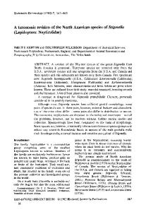
Figure 1. Global temperatures and atmospheric CO2 concentrations from 1978 – 2010 at Mona Loa, Hawaii (Northern hemisphere); time spans of Remote Sensing (RS) data sets and AMT cruises. GISS refers to the analysis by NASA’s Goddard Institute for Space Studies; HadCRUT3 refers to the third revision of analysis by the UK Met Office Hadley Centre and Climate Research Unit of the University of East Anglia; and NCDC refers to analysis by NOAA’s National Climatic Data Centre. The plot was adapted from https://ourchangingclimate.wordpress.com/2010/04/11/recent-changes-in-the-sun-co2-andglobal-average-temperature-little-ice-age-onwards/ (accessed 05/05/15)

Figure 2. Annual and seasonal coverage of AMT cruises from AMT-1 through to AMT-25 (1995-2015).

Figure 3. Atlantic CHL composites from OCTS (AMT-4) and OC-CCI (AMT-5 to AMT22) with AMT cruise tracks overlain. Including: AMT-4 (AFBS, 21/04/97 to 27/05/97); AMT-5 (BFAS, 14/09/97 to 17/10/97); AMT-14 (AFBS, 26/04/04 to 2/06/04); AMT-17 (BFAS, 15/10/05 to 28/11/05); AMT-19 (BFAS, 13/10/09 to 1/12/09); and AMT-22 (BFAS, 10/10/12 to 24/11/12).

Figure 4. Monthly climatology of sea-surface height (SSH) and surface-geostrophic-current derived from AVISO altimetry data for the Atlantic Ocean for: a) January; b) March; c) May; d) July; e) September; and f) November. The magnitude speed (background shading on a log scale) is overlaid with SSH contours at 0.2 m intervals. Grey (blue) contours show regions of positive (negative) SSH, with the zero SSH line shown in black. Current direction is shown in the green, arrow-annotated, streamlines.

Figure 5. The monthly composites of Sea Surface Salinity (SSS), derived from SMOS in the Atlantic Ocean for: a) January; b) March; c) May; d) July; e) September; and f) October.

Figure 6. Monthly climatology of Sea Surface Temperature, derived from OISST data, for January, July, March and September, with a schematic of main current systems overlain, including: 1 = North Atlantic Current (NAC); 2 = Canaries Current (CC); 3 = North Equatorial Current (NEC); 4 = Antilles Current (AntC); 5 = South Equatorial Current (SEC); 6 = Brazil Current (BC); 7 = South Atlantic Current (SAC); and 8 = Benguela Current (BenC). Breadth of arrows represents strength of flow with purple infill for low salinity currents.

Figure 7. Monthly climatology of CHL (OC-CCI data 14y composite) in the Atlantic Ocean for: a) January; b) March; c) May; d) July; e) September; and f) October.

Figure 8. Along-track AMT-22 data on: surface temperature (SST, denoted Temp in the figure); Salinity (SSS); surface Chla fluorescence (CHL); and surface Chla (CHL) derived from HPLC from discrete surface water samples taken along-track, and from measurements from an ACS. Measurements are from pumped surface-layer water (nominally 5 m depth) measured continuously by shipboard instruments, illustrating the sharp change of all variables at the gyre edges. Dashed lines show the approximate locations of the gyres edges (North Atlantic Gyre (NAG) and South Atlantic Gyre (SAG)), the South Atlantic Current (SAC), South Equatorial Current (SEC), North Equatorial Current (NEC) and North Atlantic Current (NAC) regions of NAG and SAG. Black horizontal line on the bottom plot shows the 0.15 mg m-3 CHL boundary.

Figure 9. Contoured cross-sections of Nitrate, Chla, Temp, Salinity for AMT-17, with the approximate locations of the South Atlantic Current (SAC), South Equatorial Current (SEC), North Equatorial Current (NEC) and North Atlantic Current (NAC). Figures were adapted from AMT cruise report 17, available at http://www.amt-uk.org/pdf/AMT17_report.pdf.

Figure 10. Contoured cross-sections of Nitrate, Chla, Temp, Salinity for AMT-14, with the approximate locations of the South Atlantic Current (SAC), South Equatorial Current (SEC), North Equatorial Current (NEC) and North Atlantic Current (NAC). Figures were adapted from AMT cruise report 14, available at http://www.amt-uk.org/pdf/AMT14_report.pdf.

Figure 11. (a) Shows RS climatological monthly averages of surface Chla (CHL) and PAR, and average mixed-layer depth, all averaged within each gyre (using a 0.15 mg m-3 boundary in CHL). (b) Shows seasonal cycles in estimates of the ratio of Chla at the DCM to that at the surface together with climatological monthly averages of PAR, and (c) shows seasonal cycles integrated Chla (vertically integrated within 1.5 times the euphotic depth) and depth of DCM. The ratio of Chla at the DCM to that at the surface, integrated Chla and depth of DCM were estimated by forcing the empirical model of Brewin et al. (Submitted, this issue) with climatological monthly averages of CHL within each gyre.

Figure 12. Simulations of SST (a), depth of the DCM (b), surface Chla (averages to top 40m, c) and DCM Chla (d) from the coupled ERSEM-GOTM model (Hardman-Mountford et al. 2013) at the centre of the SAG over the period 1997 to 2004.

Figure 13. Seasonal cycles of SST, Gyre Area (GA), CHL and PAR in the NAG from 1998 to 2012. Seasonal cycles were determined from averaging monthly composites of RS data within gyre boundary limits of 0.1 mg m-3 (top two figures: a and b) and 0.15 mg m-3 (bottom two figures: c and d). The timing of AMT cruises AMT-5 to AMT-21 are illustrated in the top figure.

Figure 14. Seasonal cycles of SST, Gyre Area (GA), CHL and PAR, in the SAG from 1998 to 2012. Seasonal cycles were determined from averaging monthly composites of RS data within gyre boundary limits of 0.1 mg m-3 (top two figures: a and b) and 0.15 mg m-3 (bottom two figures: c and d). The timing of AMT cruises AMT-5 to AMT-21 are illustrated in the top figure.

Figure 15.Annual anomalies and trends in the NAG for SST, CHL, GA and PAR, from 1998 to 2012, along with the Multivariate ENSO Index (MEI). Variables were spatially averaged within the NAG (using a 0.15 mg m-3 boundary in CHL).

Figure 16. Annual anomalies and trends in the SAG for SST, CHL, GA and PAR, from 1998 to 2012, along with the Multivariate ENSO Index (MEI). Variables were spatially averaged within the SAG (using a 0.15 mg m-3 boundary in CHL).

Highlights: -

We investigate the bio-physical functioning of the Atlantic Sub-Tropical Gyres.

-

We do this using AMT in situ data, remote-sensing and ecosystem modelling.

-

We define gyre boundary from a gradient in biological and physical variables.

-

Chlorophyll increases within both gyres are seen over the AMT period.