An index theorem for Toeplitz operators on partitioned manifolds (分割された多様体における Toeplitz 作用素の指数定理)

Tatsuki Seto (瀬戸 樹)

A thesis submitted for the degree of Doctor of Philosophy (Mathematical Science) in Graduate School of Mathematics, Nagoya University

January 12, 2016

Contents Chapter 1. Introduction 1.1. Summary of the main result 1.2. Background 1.3. Organization of the thesis 1.4. Notations

3 3 8 12 13

Chapter 2. Preliminaries 2.1. Properties of the Dirac operator 2.2. The index theorem for Dirac operators 2.3. Toeplitz operators

15 15 17 20

Chapter 3. 3.1. The 3.2. The 3.3. The

23 23 24 33

The Kasparov product and the index Fredholm index and K theory Kasparov product cyclic cohomology and Connes’ pairing

Chapter 4. The Roe-Higson index theorem 4.1. The Roe algebra 4.2. The odd index 4.3. Roe’s cyclic one-cocycle associated to a partition 4.4. The Roe-Higson index theorem 4.5. Applications

35 35 40 41 45 49

Chapter 5. Main theorem 5.1. Definition of the index class 5.2. Main theorem 5.3. Wrong way functoriality 5.4. Remarks on the odd index class 5.5. Calculation of the index class 5.6. Proof of Main theorem 5.7. Example

51 51 52 53 55 56 63 73

Appendix A. The Hilbert transformation

77

Bibliography

81 1

CHAPTER 1

Introduction 1.1. Summary of the main result Let M be a complete Riemannian manifold and S → M a Hermitian vector bundle on M . J. Roe [34] introduced a non-unital C ∗ -algebra C ∗ (M ) = X , where X denotes the algebra of bounded integral operators on L2 (M, S) which have smooth kernel functions supported within a bounded neighborhood of the diagonal of M × M . It is called the Roe algebra. One has K1 (C ∗ (M )) = π0 (GL∞ (C ∗ (M ))) by definition, where π0 stands for the set of connected components. It turns out to be an abelian group. Let D be the Dirac operator acting on a Clifford bundle S. Roe also defined an odd index for D, ind(D), as an element in K1 (C ∗ (M )). It is known that the odd index is represented by the Cayley transformation of D: [

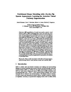
] D−i ind(D) = ∈ K1 (C ∗ (M )). D+i Assume that there exist two submanifolds with boundary, M + and M , of the same dimension as M that satisfy the conditions M = M + ∪ M − and M + ∩ M − = ∂M + = ∂M − . Set N = M + ∩ M − , which is a submanifold of M of codimension one. We call such M a partitioned manifold if such N is a closed manifold, that is, N is a compact, oriented manifold without boundary; see below Figure 1.1.1. Denote by Π the characteristic function of M + and set Λ = 2Π − 1. Π and Λ act on L2 (M, S) as a multiplication operator, respectively. −

Figure 1.1.1. Partitioned manifold 3

4

1. INTRODUCTION

In this setting, Roe also defined a cyclic 1-cocycle ζ: 1 ζ(A, B) = Tr(Λ[Λ, A][Λ, B]) 4 for A, B ∈ A , where A is a certain Banach algebra, which is dense in C ∗ (M ) and the inclusion map induces an isomorphism of K1 groups: K1 (A ) ∼ = K1 (C ∗ (M )). Then ζ defines a linear map ζ∗ : K1 (C ∗ (M )) → C, which is essentially given by substituting an element in A in ζ. This coincides with Connes’ pairing of a cyclic cohomology with K theory; see Subsection 3.3.2. On the other hand, it is known that there is a Z2 -graded Dirac operator DN on S|N with the grading the Clifford multiplication of ν. Here, ν is the unit normal vector field; see Figure 1.1.1. DN is an odd + operator with respect to the grading, so DN splits the positive part DN − and the negative part DN . Roe [34] proved the following formula in 1988: 1 + ζ∗ (ind(D)) = − index(DN ). 8πi N. Higson [26] proved this formula with a simplified proof in 1991, after Roe’s work. We shall call the formula the Roe-Higson index theorem from now on. It is known that the Fredholm index of an elliptic differential operator on an odd-dimensional closed manifold is 0; see [4, Proposition 9.2]. + Thus we have index(DN ) = 0 when N is of odd dimension. Therefore, the Roe-Higson index ζ∗ (ind(D)) is trivial when M is of even dimension. However, the value ζ∗ (x) is non trivial for a general x ∈ K1 (C ∗ (M )). In this thesis, we shall study such values on even-dimensional mani+ folds M replacing index(DN ) by the Toeplitz index, which is a counterpart of the Roe-Higson index theorem on odd-dimensional manifolds. To be more precise, we replace two parts, ind(D) and the Dirac op+ ˆ erator DN by an index class Ind(ϕ, D) = [ϕ]⊗[D] and the Toeplitz operator on N , respectively.

dim M odd index operator on N

Main theorem even Ind(ϕ, D) Toeplitz operator Tϕ|N

Roe-Higson index theorem odd ind(D) + Dirac operator DN

The odd index Ind(ϕ, D) and the associated Toeplitz operator is defined as follows. Let D be the graded Dirac operator on S = S + ⊕ S − and ϵ the grading operator. Denote by Cw (M ) the C ∗ -algebra

1.1. SUMMARY OF THE MAIN RESULT

5

generated by bounded smooth functions on M with bounded gradient. Then we can define [D] ∈ KK 0 (Cw (M ), C ∗ (M )) and [ϕ] ∈ K1 (Cw (M )) for ϕ ∈ GLl (Cw (M )). By using the Kasparov product ˆ : K1 (Cw (M )) × KK 0 (Cw (M ), C ∗ (M )) → K1 (C ∗ (M )), ⊗ ˆ we obtain Ind(ϕ, D) = [ϕ]⊗[D] by definition. More explicitly, it is given by [ [ ] [ ]] ϕ 0 1 0 Ind(ϕ, D) = D D ∈ K1 (C ∗ (M )), 0 1 0 ϕ−1 where the bounded operator D on L2 (M, S) is defined by D = (D + ϵ)(D2 + 1)−1/2 . Next we construct the Toeplitz operator. Index theory for Toeplitz operators on closed manifolds is developed by P. Baum and R. G. Douglas [7], [8]. Set SN = S + |N and let DN : L2 (N, SN ) → L2 (N, SN ) be the Dirac operator on SN . It is well known that the spectrum of DN consists of only real eigenvalues with finite multiplicity. Let H+ ⊂ L2 (N, SN ) be the closed subspace generated by all eigenvectors for DN corresponding to non-negative eigenvalues. Denote by P the projection onto H+ . Let ψ ∈ GLl (C(N )), which can be considered as a continuous mapping ψ : N → GLl (C) at the same time. The Toeplitz operator Tψ with symbol ψ is defined to be a compression of the multiplication operator on H+ . Namely, we define Tψ : H+l → H+l to be Tψ s = P ψs. We note that Tψ is a Fredholm operator since ψ takes the values in GLl (C). We shall study ζ∗ (Ind(ϕ, D)) and prove that it is equal to the Fredholm index of a Toeplitz operator on N . Recall that Cw (M ) is the C ∗ algebra generated by bounded smooth functions on M with bounded gradient. Then an element ϕ ∈ Ml (Cw (M )) can be considered as a continuous mapping ϕ = [ϕij ] : M → Ml (C) such that ϕij ∈ Cw (M ) at the same time. Thus an element ϕ ∈ Ml (Cw (M )) belongs to GLl (Cw (M )) if and only if ϕ takes the values in GLl (C) and one has ϕ−1 ∈ Ml (Cw (M )), where ϕ−1 is defined by ϕ−1 (x) = ϕ(x)−1 . The precise statement of the main theorem is as follows: Main Theorem (see Theorem 5.2.1). Let M be a complete Riemannian manifold partitioned by N as previously. Let S → M be a graded Clifford bundle with grading ϵ and denote by D the graded Dirac operator of S. Take ϕ ∈ GLl (Cw (M )). Then the following formula holds: 1 index(Tϕ|N ), ζ∗ (Ind(ϕ, D)) = − 8πi where Tϕ|N is the Toeplitz operator with symbol ϕ|N : N → GLl (C).

6

1. INTRODUCTION

In particular, if ϕ : M → GLl (C) is a bounded smooth mapping with bounded gradient and ϕ−1 : M → GLl (C) is also bounded, then we have ϕ ∈ GLl (Cw (M )). Here, bounded means the supremum on M of the norm on Ml (C) is finite. Applying the topological formula for Toeplitz operators proved by Baum-Douglas [7], [8], we obtain the following: Corollary (see Corollary 5.2.2). Let M be a complete Riemannian manifold partitioned by N as previously. Denote by Π the characteristic function of M + . Let S → M be a graded Clifford bundle with grading ϵ and denote by D the graded Dirac operator of S. Assume that ϕ ∈ C ∞ (M ; GLl (C)) is bounded with bounded gradient and ϕ−1 is also bounded. Then one has ( [ ] ) −1 ϕ 0 2 l 2 l index Π(D + ϵ) (D + ϵ)Π : Π(L (M, S)) → Π(L (M, S)) 0 1 ∫ π ∗ Td(T N ⊗ C)ch(S + )π ∗ ch(ϕ). = S∗N

The idea of the proof is as follows. Firstly, we calculate the Kasˆ parov product [ϕ]⊗[D] by using the Cuntz picture of [D]. Secondly, we calculate ζ∗ (Ind(ϕ, D)) explicitly by using the Hilbert transformation and a homotopy of Fredholm operators in the case for M = R × N and ϕ = 1 ⊗ ψ with ψ ∈ C ∞ (N ; GLl (C)). Finally, we reduce the general case to R × N by applying a similar argument in Higson [26]. Set M = R × N and assume that N is of odd dimension. In this case, the main theorem is derived from the Roe-Higson index theorem by applying the suspension homomorphism formally. Let D be the Dirac operator on M and take a mapping ϕ : M → GLl (C). Then they determine elements [[D]] ∈ KK 0 (M, pt) and [[ϕ]] ∈ KK 1 (M, M ), ˆ with σ the suspension respectively. By using the Kasparov product ⊗, homomorphism and e an induced mapping by the map to one point, we have the following commutative diagram: KK 1 (M, M ) × KK 0 (M, pt)

/ KK 0 (M × S 1 , M × S 1 ) × KK 1 (M × S 1 , pt)

ˆ ⊗



KK 1 (M, pt) 

KK 1 (M × S 1 , pt)

σ

KK 0 (N, pt) 

ˆ ⊗



e

Z



σ

KK 0 (N × S 1 , pt) 

e

Z

1.1. SUMMARY OF THE MAIN RESULT

([[ϕ]], [[D]])  _

ˆ ⊗



ˆ [[ϕ]]⊗[[D]] _

/ ([[Eϕ ]], [[D 1 ]]) _ M ×S ˆ ⊗



ˆ [[Eϕ ]⊗[[D M ×S 1 ]] _

σ



ˆ [[ϕ|N ]]⊗[[D N ]] _ 

e

index(Tϕ|N )

7

σ



[[Dϕ|N ]] _ 

e

index(Dϕ|N )

Here, Eϕ is the vector bundle clutched by ϕ and Dϕ|N the Dirac operator on N × S 1 twisted by Eϕ|N . To be precise, we set Eϕ = (M × [0, 1] × Cl )/ ∼ with (x, 0, v) ∼ (x, 1, ϕ(x)v). By the second column and the Roe-Higson index theorem, we have e ◦ σ = ζ∗ ◦ A, where A : KK 1 (M, pt) → K1 (C ∗ (M )) is the map defining the odd index called ˆ ˆ the assembly map. Thus, we have ζ∗ (A([[ϕ]]⊗[[D]])) = e(σ([[ϕ]]⊗[[D]])) = index(Tϕ|N ), which is a statement of the main theorem for M = R × N . This formal argument is correct if ϕ is an element in GLl (C0 (M )) since the above KK groups are defined as KK 1 (M, pt) = KK 1 (C0 (M ), C), for instance. However, if ϕ were chosen as an element in GLl (C0 (M )), ϕ should take a constant value outside a compact set of M . This implies that ϕ|N is homotopic to a constant function in GLl (C(N )) and thus index(Tϕ|N ) should vanish. Therefore, in order to obtain non-trivial index, we have to employ a larger algebra than C0 (M ). Higson [25] introduced such a C ∗ -algebra Ch (M ) that contains C0 (M ), which is now called the Higson algebra. It plays an important role in a K-homological proof of the Roe-Higson index theorem. The Higson algebra is defined as follows: Ch (M ) is the C ∗ -algebra generated by all smooth and bounded functions defined on M of which gradient is vanishing at infinity [25, p.26]. Ch (M ) contains C0 (M ) as an ideal and is contained in Cw (M ) by definition. Given ψ ∈ C ∞ (N ), we note that ϕ = 1 ⊗ ψ does not belong to Ch (M ) in general. Thus the Higson algebra is not large enough to prove our main theorem. On the other hand, we have ϕ ∈ Cw (M ). Moreover, Cw (M ) is the largest C ∗ -algebra A for which we can define [D] as an element in KK 0 (A, C ∗ (M )). They are reasons why we introduced the C ∗ -algebra Cw (M ) in our main theorem. Last but not least, the Roe-Higson index theorem is generalized by M. E. Zadeh [37] and T. Schick and Zadeh [44], for instance. However, they treat N of even dimension, essentially.

8

1. INTRODUCTION

1.2. Background Let Σ be a closed Riemannian surface, where closed means compact, oriented and without boundary. By the classification theorem of closed surfaces, Σ is classified by the number of holes. The number g(Σ) is called the genus of Σ. Denote by K : Σ → R the Gaussian curvature of Σ. The Gauss-Bonnet theorem gives a relationship of g(Σ) and K: ∫ 1 2 − 2g(Σ) = K ∗ 1. 2π Σ Here, ∗ is the Hodge star operator. The left hand side 2 − 2g(Σ) is called the Euler number χ(Σ) of Σ. We can see this formula connects a global invariant and a local invariant. Moreover, we can also see this formula connects an analytic invariant and a geometric invariant as described later. The Gauss-Bonnet theorem is generalized by C. B. Allendoerfer and A. Weil [1] in 1943 to closed Riemannian manifolds N of even dimension. Their proof is using the embedding into a Euclidean space of a sufficiently high dimension. After that, S. Chern [13] proved the generalized Gauss-Bonnet theorem by using differential forms without embedding into a Euclidean space in 1944. By using the Chern-Weil theory [14], its generalization is formulated as follows: χ(N ) =

dim ∑N j=0

∫ (−1) H (N ; C) = j

j

e(T N ), N

where e(T N ) is the Euler class of the tangent bundle T N . We can see this formula also connects a global invariant and a local invariant or an analytic invariant and a geometric invariant. As same as the above formulas, the Riemann-Roch-Hirzebruch theorem and the Hirzebruch signature theorem is also connecting such invariants. The Riemann-Roch-Hirzebruch theorem connects the Euler number of a Dolbeault complex and the Todd class (we can expand it a polynomial of Chern classes). The Hirzebruch signature theorem connects the signature of the intersection form and the L class (we can expand it a polynomial of Pontrjagin classes). In 1963, M. F. Atiyah and I. M. Singer [2] presented the index theorem for elliptic differential operators on closed manifolds N . In particular, above Euler numbers or signatures are equal to the Fredholm index of Dirac operators D defined by the following: index(D) = dim Ker(D) − dim Ker(D∗ ) ∈ Z.

1.2. BACKGROUND

9

This quantity is calculated by the dimension of the solution space of differential equations Ds = 0 and D∗ s = 0. So index(D) is a global and analytic number. For example, by using the Hodge theory, we can see the Euler number χ(N ) in the Gauss-Bonnet-Chern theorem is equal to index((d + d∗ )+ ), where d is the exterior differential for differential forms and upper + means the restriction to the set of differential forms of even degree. On the other hand, the notion of Dirac operators is a generalization of the canonical Dirac operator for a spin manifold. In this case, the Atiyah-Singer formula is as follows: ∫ + ˆ N ), index(D ) = A(T N +

where upper means the restriction of the canonical Dirac operator to ˆ N ) is a characteristic class of T N the set of positive spinors and A(T called Aˆ class (we can expand it a polynomial of Pontrjagin classes). We often assume the Dirac operator D acting on S is graded, that is, D is an odd operator with respect to a Z2 -grading of S like above examples. Atiyah-Singer generalized their index theorem for elliptic pseudodifferential operators by using topological K-theory [3]. There are a lot of advantages of this generalization. For example, we can get a nontrivial index for odd dimensional manifolds since every elliptic differential operator has trivial index, that is, index = 0; see [4, Proposition 9.2]. The most typical example of an elliptic pseudo-differential (not differential) operator is given by the Toeplitz operator Tϕ . As an example, we assume N = S 1 is a unit circle, the simplest closed manifold. Let ϕ ∈ C ∞ (S 1 ) be a smooth function with ϕ(x) ̸= 0 for x ∈ S 1 and H+ the Hardy space, that is, the set of L2 -boundary value functions on S 1 of holomorphic functions on the unit disk. Denote by P the projection onto H+ . Then we define the Toeplitz operator Tϕ : H+ → H+ to be Tϕ f = P ϕf . In this case, Dϕ = Tϕ ⊕ 1 on L2 (S 1 ) = H+ ⊕ H+⊥ is an elliptic pseudo-differential operator of order 0 and we have index(Dϕ ) = index(Tϕ ). Then the Atiyah-Singer index formula gives the Gohberg-Krein formula [23]: index(Tϕ ) = − deg(ϕ), where deg means the winding number. More generally, index theory for Toeplitz operators on the general N is developed by P. Baum and R. G. Douglas [7], [8]; see also Subsection 2.3. Thanks to the K-theoretical approach, we can generalize the notion of the Fredholm index. Indeed, Atiyah-Singer defined the index for equivariant elliptic operators with the action of a group in [3] and the

10

1. INTRODUCTION

index for families of elliptic operators in [5]. In particular, the index of a family of elliptic operators {Dx }x∈X parametrized by a compact Hausdorff space X is defined as an element in K(X), that is, it is a formal difference of vector bundles over X. If the dimension of Ker(Dx ) is independent of x ∈ X, then it is represented by the following: index({Dx }) = [∪Ker(Dx )] − [∪Ker(Dx∗ )] ∈ K(X). Since the category of vector bundles on X and that of finitely generated projective C(X)-modules are categorical equivalence by the Swan theorem, we have K(X) ∼ = K0 (C(X)). Here, K0 (C(X)) is a K0 group of C(X), that is, K0 (C(X)) is the group generated by the stable homotopy class of idempotents in M∞ (C(X)). Thus we have index({Dx }) ∈ K0 (C(X)). By using the above point of view, we assume that a generalized index is an element in K groups for algebras. We use K groups for operator algebras since it has several properties compatible with geometry, for example, it satisfies K1 (C(X)) ∼ = K −1 (X). Its generalization is called an index class. We can also assume that the ordinary index is an element in K0 (K), where K is the C ∗ -algebra of all compact operators on a fixed countably infinite dimensional Hilbert space. It is provided by the Atkinson theorem; see Section 3.1. By the way, there is another (but related) approach for the identification of the Fredholm index with an element in K0 (K). Let D be the graded Dirac operator on a closed manifold. Then we have [eD ] − [p] ∈ K0 (K), where we set [ ] [ ] 1 D− 0 0 2 −1 eD = (D + 1) and p = . D+ D+ D− 0 1 eD is called the graph projection of D. Moreover, by using an isomorphism Tr∗ : K0 (K) ∼ = Z which is defined essentially by substituting an operator in the trace Tr, we have index(D+ ) = Tr∗ ([eD ] − [p]). We note that we can see the isomorphism Tr∗ is defined by Connes’ pairing [18] of the cyclic 0-cocycle Tr with K0 (K). By using an index class, we can study an index problem for more general spaces. For example, non-compact manifolds, foliated manifolds and Hilbert module bundles. We are interested in non-compact, complete Riemannian manifolds in this thesis. In this case, we can not define the ordinary Fredholm index in general. For example, the Dirac operator −id/dt on R is not Fredholm. Thus we should define a generalized index.

1.2. BACKGROUND

11

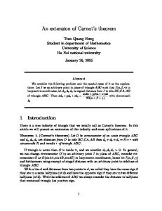
Let M be a complete Riemannian manifold and D the Dirac operator on M . J. Roe [34] defined the C ∗ -algebra C ∗ (M ), which is called the Roe algebra, and the odd index ind(D) ∈ K1 (C ∗ (M )). By using this odd index, Roe [34] proved an index theorem for a complete manifold partitioned by a closed hypersurface N like Figure 1.2.1: M = M − ∪N M + .

Figure 1.2.1. Partitioned manifold The statement of Roe’s theorem is as follows. By using the partition of M , Roe defined the cyclic 1-cocycle ζ, which is called the Roe cocycle. Recall that A. Connes [18] defined the pairing of a cyclic cohomology with a K group. Roe proved Connes’ pairing of ζ with ind(D) is equal + to the Fredholm index of the restricted Dirac operator DN on N up to a certain constant multiple: (♠)

+ ⟨ind(D), ζ⟩ = index(DN ),

where the grading of DN is defined by the Clifford action of the unit normal vector field ν. Higson [26] gave a short proof of a variation of Roe’s theorem after Roe’s work. Thus we call the formula (♠) the Roe-Higson index theorem in this thesis. In fact, let Π be the characteristic function of M + and φ ∈ C ∞ (M ) a smooth function such that we have φ = Π on the complement of a compact set in M . We identify φ with a multiplication operator of it. Higson proved + index(1 − φ + φ(D − i)(D + i)−1 ) = index(DN ).

Roe’s original proof is using K-theoretical argument. On the other hand, Higson’s proof is based on a calculation of the dimension of the solution space of a first order ordinary linear differential equation. Firstly, he proved the case when M = R × N by calculation of its dimension. Secondly, he reduced the proof for a general partitioned manifold M to the case when M = R × N . Since the Fredholm index of the Dirac operator on a closed manifold of odd dimension is 0, the right hand side of the Roe-Higson index theorem is trivial when M is of even dimension. Thus, this theorem is a theorem when M is of odd dimension, essentially.

12

1. INTRODUCTION

The Roe-Higson index theorem is generalized by some researchers. U. Bunke’s Callias-type index theorem [12] covers the Roe-Higson index theorem by using the point of view of Higson. P. Siegel [39] generalized when the Dirac operator is equivariant with an action of a discrete group and a manifold has a certain geometric condition. M. E. Zadeh [43, 44] generalized for Hilbert module bundles on a partitioned manifold of odd dimension. S. Kamimura [28] generalized for a product manifold Rp × N even (R × N is a partitioned manifold). T. Shick and Zadeh [37] generalized for a p-multi-partitioned manifold M with dim M − p = even (“dim M − p = odd” implies trivial index). Siegel [39] also treats the case when a multi-partitioned manifold has a certain geometric condition. Here, Rp × N is a typical example of a p-multi-partitioned manifold. 1.3. Organization of the thesis In Section 2, we recall basic properties of the Dirac operator. We also recall the index theorem for Dirac operators and Toeplitz operators. In Section 3, we review a generalization of the notion of the analytic index in terms of noncommutative geometry in the required range. In Section 4, we review the Roe-Higson index theorem. Definitions of the Roe algebra, the Roe cocycle and its pairing are contained in this section. In Section 5, we discuss the main theorem. As the appendix, we review a part of properties of the Hilbert transformation. These properties are used in Sections 4 and 5. Acknowledgments I deeply grateful to my advisor, Professor Hitoshi Moriyoshi, for his valuable mathematical and non-mathematical suggestions and teachings. I would also grateful to Professor Toshikazu Natsume for his valuable comments on the thesis. I also would like to thank my parents for their financial support for my study.

1.4. NOTATIONS

13

1.4. Notations Numbers. N The set of positive integers. Z+ The set of non-negative integers. Z The set of integers. Q The set of rational numbers. R The set of real numbers. C The set of complex numbers. Z2 Z2 = Z/2Z. Classes of maps. C It means C r -class. We use also C = C 0 . ∞ Cc It means compactly supported C ∞ -class. C0 It means continuous and vanishing at infinity. Cb It means continuous and bounded. 2 L It means square integrable. F (X; A) The set of A-valued functions defined on X of class F . We use also F (X) = F (X; C). F (X, E) The set of sections of a bundle E → X of class F . S (Rn ) The set of rapidly decreasing functions on Rn . ′ n S (R ) The topological dual of S (Rn ). K(X, Y ) The set of compact operators from X to Y . We use also K(X) = K(X, X). K The C ∗ -algebra of compact operators on a Hilbert space of countably infinite dimension. L(X, Y ) The set of bounded operators from X to Y . We use also L(X) = L(X, X). r

Not often used constructions. E⊠F

The exterior tensor product of two vector bundles E → X1 and F → X2 : E ⊠ F = p∗1 E ⊗ p∗2 F , where pi : X1 × X2 → Xi is the projection. A △ B The symmetric difference of A and B: A △ B = (A ∪ B) \ (A ∩ B).

14

1. INTRODUCTION

Operator K groups. Let A be a Banach algebra. The unital algebra adjoining a unit of A: A+ = A ⊕ C. The suspension of A: SA = C0 (R) ⊗ A. The set of n × n matrices of A. ∪ The inductive limit of Mn (A): M∞ (A) = ∞ n=1 Mn (A). The set of idempotents of Mn (A). The K0 group of A: K0 (A) = {[e] − [f ] ; e, f ∈ In (A+ ) and e − f ∈ Mn (A)}. GLn (A+ ) The set of n × n invertible matrices of A+ . GLn (A) GLn (A) = {u ∈ GLn (A+ ) ; u − 1 ∈ Mn (A)}. ∪ GL∞ (A) The inductive limit of GLn (A): GL∞ (A) = ∞ n=1 GLn (A). K1 (A) The K1 group of A: K1 (A) = π0 (GL∞ (A)). Let A be a C ∗ -algebra. Pn (A) The set of projections of Mn (A). Un (A+ ) The set of n × n unitary matrices of A+ . Un (A) Un (A) = {u ∈ Un (A+ ) ; u − 1 ∈ Mn (A)}. ∪ U∞ (A) The inductive limit of Un (A): U∞ (A) = ∞ n=1 Un (A). A+ SA Mn (A) M∞ (A) In (A) K0 (A)

CHAPTER 2

Preliminaries In this chapter, we recall basic properties of the Dirac operator on a complete Riemannian manifold and the index theorem for Dirac operators on a closed manifold. Furthermore, we also recall the index theorem for Toeplitz operators since the index of the Dirac operator on odd-dimensional manifolds is always trivial. There are a lot of helpful references for topics in this chapter, for example, [8], [9], [27], [31] and [36]. 2.1. Properties of the Dirac operator Let M be a complete Riemannian manifold of dimension n without boundary. Let (S, h) → M be a Clifford bundle, that is, S is a Hermitian vector bundle equipped with a metric connection ∇S and an action c ∈ C ∞ (M, Hom(Cl(T M ), End(S))) of the complex Clifford module bundle Cl(T M ) of the tangent bundle T M such that • h(c(X)s, t) + h(s, c(X)t) = 0, • ∇SX (c(Y )s) = c(∇X Y )s + c(Y )∇SX s, for any X, Y ∈ C ∞ (M, T M ) and s, t ∈ C ∞ (M, S); see [36, Definition 3.4]. By using ∇S and c, we can define the Dirac operator of S as a composition of these maps: ∇S

♯⊗id

D : C ∞ (M, S) −→ C ∞ (M, T ∗ M ⊗S) −→ C ∞ (M, T M ⊗S) −→ C ∞ (M, S). c

Here, ♯ : T ∗ M → T M is the isomorphism defined by using the Riemannian metric of M . We often identify T ∗ M with T M by using ♯. By definition, the Dirac operator is a globally defined first-order elliptic differential operator with the principal symbol ic(ξ). We can write D=

n ∑

c(ei )∇Sei ,

i=1

where e1 , . . . en is a local orthonormal frame of T M . We often assume a Clifford bundle is Z2 -graded, that is, S = S + ⊕ S − is a Z2 -graded Hermitian vector bundle, ∇S is an even operator 15

16

2. PRELIMINARIES

and c(v) for v ∈ T M is an odd operator. When a Clifford bundle S is Z2 -graded, its Dirac operator is an odd operator by definition: [ ] 0 D− D= : C ∞ (M, S + )⊕C ∞ (M, S − ) → C ∞ (M, S + )⊕C ∞ (M, S − ) D+ 0 We often say graded means Z2 -graded. Example 2.1.1. ∧ • We can consider that the exterior tensor product ∗ T ∗ M ⊗ C of the cotangent bundle T ∗ M is a Clifford bundle. In this case, the Dirac operator D is D = d + d∗ , where d is the exterior differential for differential forms on M . • Let W → M be a holomorphic vector bundle with∧the canonical connection on a Hermitian manifold M . Then ∗ (T 0,1 M )∗ ⊗ W bundle and its Dirac operator D is D = √ is a Clifford ∗ 2(∂¯W + ∂¯W ) + A for a certain endomorphism A ∈ End(S). In particular, if M is a K¨ahler manifold, then we have A = 0. • Let M admits a spin structure. In this case, the spin bundle ∆ defined by its spin structure is a Clifford bundle. In this case, the canonical spinor Dirac operator of ∆ is the Dirac operator in our definition. If M is of even dimension, then ∆ is Z2 -graded by the decomposition of positive and negative spinors. • Let D : C ∞ (M, S) → C ∞ (M, S) be the Dirac operator and E → M a Hermitian vector bundle with a metric connection. We assume a connection of S ⊗E is the tensor product connection. Then S ⊗ E is a Clifford bundle with the Clifford action c ⊗ 1. We denote by DE the Dirac operator on S ⊗ E. DE is called the Dirac operator twisted by E. Since the boundary of M is empty and S has the compatibility conditions, the Dirac operator D is a formally self-adjoint operator. Because of the completeness of the Riemannian metric of M , we have the following important property. Theorem 2.1.2. [15] D is an essentially self-adjoint operator, that ¯ on L2 (M, S). is, D has a self-adjoint closed extension D ¯ by D in the sequel. Denote by H 1 (M, S) the We often denote D domain of D. This space is a Hilbert space by the graph norm of D, that is, the Sobolev first inner product ⟨u, v⟩H 1 = ⟨u, v⟩L2 + ⟨Du, Dv⟩L2 defines a complete norm on H 1 (M, S). H 1 (M, S) is called the (first) Sobolev space. More generally, we can define higher order Sobolev

2.2. THE INDEX THEOREM FOR DIRAC OPERATORS

17

spaces for k ∈ N as follows: H k (M, S) = {u ∈ H 1 (M, S) ; ∥u∥H k < +∞}. Here, the Sobolev k-th norm ∥ · ∥H k is defined by the following Sobolev k-th inner product: ⟨u, v⟩H k = ⟨u, v⟩L2 +

k ∑

⟨Dr u, Dr v⟩L2 .

r=1 k

H (M, S) is a Hilbert space by the Sobolev k-th norm. Set H 0 (M, S) = L2 (M, S). We can define these Sobolev type spaces more general order s ∈ R. However, we use only the case when k ∈ Z+ . The last of this subsection, we collect well-known properties of Sobolev spaces which we use. Denote by H k (K, S) the subspace of H k (M, S) with supported by a compact set K ⊂ M . Since the principal symbol of the Dirac operator D is ic(ξ), D is a first order elliptic differential operator. Thus, because of the elliptic estimate, our Sobolev spaces coincide with ordinary Sobolev spaces on a compact set, that is, H k (K, S) coincides with the set of all k-th derivatives are of L2 -class. Theorem 2.1.3. • The inclusion H l (M, S) → H k (M, S) is continuous for l ≥ k. • D : H k+1 (M, S) → H k (M, S) is continuous. • (The Sobolev embedding theorem) Let r ∈ Z+ and k > n/2 + r and assume K ⊂ M is a compact subset. If u ∈ H k (K, S), then we have u ∈ C r (M, S) and there exists C = C(n, r, s) > 0 such that we have ∥u∥r,∞ ≤ C∥u∥H s . Here, ∥ · ∥r,∞ is the uniform C r norm. • (The Rellich lemma) Assume K ⊂ M is a compact subset and l > k. Then the inclusion H l (K, S) → H k (M, S) is a compact operator. • (The Maurin theorem) Assume K ⊂ M is a compact subset and r > dim M/2. Then the inclusion H k+r (K, S) → H k (M, S) is of Hilbert-Schmidt class. 2.2. The index theorem for Dirac operators Let S → N be a Clifford bundle on a closed Riemannian manifold N and D the Dirac operator of S, where closed means compact, oriented and without boundary. Since D is self adjoint, the spectrum of D is contained in R. Thus, resolvent operators (D ± i)−1 are bounded on L2 (N, S). Furthermore, we can see (1+D2 )−1 = (D +i)−1 (D −i)−1 is a bounded operator as H k (N, S) → H k+2 (N, S). Thanks to the Rellich lemma and the compactness of N , (1 + D2 )−1 is a compact operator

18

2. PRELIMINARIES

on H k (N, S). By using the spectral decomposition of the self-adjoint compact operator (1 + D2 )−1 ∈ K(L2 (N, S)), we can show that the set of spectra of closed operator D on L2 (N, S) does not have a limit point in R and contains only real eigenvalues with finite multiplicity. Moreover, the definition of Sobolev spaces and the Sobolev embedding theorem imply all eigensections are smooth. In particular, the dimension of the kernel of D ∈ L(H k+1 (N, S), H k (N, S)) is independent of k. We note that D · D(D2 + 1)−1 = idH k − (D2 + 1)−1 and D(D2 + 1)−1 · D = idH k+1 − (D2 + 1)−1 . By above observations, D is a Fredholm operator and we can define the Fredholm index of D. We recall the notion of a Fredholm operator. Theorem 2.2.1 (The Atkinson theorem). Let H and H ′ are two Hilbert spaces and T : H → H ′ a bounded operator. Then the followings are equivalent: • T is a Fredholm operator, that is, the image of T is closed and we have dim Ker(T ) < ∞ and dim Coker(T ) < ∞. • There exists S ∈ L(H ′ , H) such that ST −1 ∈ K(H), T S −1 ∈ K(H ′ ). Let T ∈ L(H, H ′ ) be a Fredholm operator. We define the Fredholm index of T as follows: index(T ) = dim Ker(T ) − dim Coker(T ) ∈ Z. The Fredholm index of D ∈ L(H k+1 (N, S), H k (N, S)) is always 0 since D is self adjoint. In order to avoid this vanishing, we assume S is a Z2 -graded Clifford bundle. In this setting, D+ ∈ L(H k+1 (N, S + ), H k (N, S − )) is also Fredholm and the Fredholm index of D+ is independent of the choice of k since we have dim Coker(D+ ) = dim Ker(D− ). Summarizing the above, we can define the Fredholm index of D+ : index(D+ ) = dim Ker(D+ ) − dim Ker(D− ) ∈ Z. The Atiyah-Singer index theorem for the Dirac operator calculates this quantity by geometrical information. By the Chern-Weil theory, a differential form [ ( )]1/2 R/4πi ˆ N ) = det A(T sinh R/4πi 4∗ defines an element in the de Rham cohomology group HdR (N ; C), where R is a Riemannian curvature tensor of N . This is called the Aˆ class of T N . In fact, Aˆ class defines an element in H 4∗ (N ; Q) since we can expand it by a polynomial over Q of Pontrjagin classes as follows: ˆ N ) = 1− 1 p1 + 1 (−4p2 +7p2 )− 1 (16p3 −44p1 p2 +31p3 )+· · · A(T 1 1 24 5760 967680

2.2. THE INDEX THEOREM FOR DIRAC OPERATORS

19

On the other hand, we recall the spinor representation is defined by the restriction of the irreducible representation of the complex Clifford algebra. So a Clifford bundle S is equivalent locally to a tensor product of the spinor bundle ∆|U of U with a coefficient vector bundle E|U ˆ U . Of course, if M is spin, then this equivalence locally: S|U ∼ = ∆|U ⊗E| holds globally. When S is Z2 -graded, E|U has been often Z2 -graded. Let K be the curvature of S and set 1∑ RS (ei , ej ) = g(R(ei , ej )ek , el )c(ek )c(el ). 4 k,l Then RS is a globally defined operator and RS |U defines the curvature of ∆|U . So F S = K − RS is a globally defined operator and F S |U defines the curvature of E|U . By using the Chern-Weil theory again, a differential form chs (S/∆) = trs (exp(−

1 S F )) 2πi

2∗ defines an element in HdR (N ; C). Here, we define trs (A0 + A1 ) = tr(A0 ) − tr(A1 ) for A0 is an operator on the positive part and A1 is an operator on the negative part. We finished the preparation of the ingredients in the index formula. The actual formula as follows:

Theorem 2.2.2 (Atiyah-Singer). [2] Let S → N be a Z2 -graded Clifford bundle on a closed Riemannian manifold N and D the Dirac operator of S. Then the following formula holds: ∫ + ˆ N )chs (S/∆). index(D ) = A(T Example 2.2.3.

N

∧ • Assume that D is equal to d+d∗ on a Clifford bundle ∗ T ∗ N ⊗ C with the Z2 -grading the parity of differential forms. Then the Atiyah-Singer formula implies the Gauss-Bonnet-Chern formula: ∫ + χ(N ) = index((d + δ) ) = e(T N ). √

N

∗ • Assume∧that D is equal to 2(∂¯W + ∂¯W ) + A on a Clifford bundle ∗ (T 0,1 N )∗ ⊗ W on a Hermitian manifold N with the Z2 -grading the parity of differential forms. Then we have ∗ + index(D+ ) = index((∂¯W + ∂¯W ) ). Therefore the Atiyah-Singer

20

n ∑

2. PRELIMINARIES

formula implies the Riemann-Roch-Hirzebruch formula: ∫ j 0,j ∗ + ¯ ¯ (−1) dim H (N, W ) = index((∂W + ∂W ) ) = Td(T N )ch(W ). N

j=0

It seems that the proof of this formula for a general Hermitian manifold is only known this implication by the Atiyah-Singer formula. • Assume that DE is a spinor Dirac operator twisted by an ungraded Hermitian vector bundle E on spin manifold N of even dimension. Then DE is Z2 -graded by the decomposition of positive and negative spinors. Then the Atiyah-Singer formula becomes more clear: ∫ + ˆ N )ch(E). index(DE ) = A(T N

2.3. Toeplitz operators Let S → N be a Clifford bundle on a closed Riemannian manifold N and D be the Dirac operator of S. Let assume N is of odd dimension. By the Atiyah-Singer formula, we can see index(D+ ) = 0. Moreover, the Fredholm index of every elliptic differential operator on odd-dimensional closed manifold is always 0; see, for instance [4, Proposition 9.2]. In order to avoid this vanishing, we should use non “elliptic differential” operators. We use elliptic pseudo-differential operators. The Toeplitz operator which is defined as follows gives the most typical example of elliptic pseudo-differential operators. Let H+ be the subspace of L2 (N, S) generated by all eigensections of D corresponding to a non-negative eigenvalue. Denote by P the orthogonal projection onto H+ . Let ϕ ∈ C(N ; Ml (C)) be a matrix valued continuous function on N . By using these data, we define the Toeplitz operator as follows: Definition 2.3.1. [8, p.146] Define the bounded linear operator Tϕ : H+l → H+l by Tϕ s = P (ϕs). We call Tϕ the Toeplitz operator (with symbol ϕ). Example 2.3.2. We assume N = S 1 = R/2πZ, the unit circle, S = S 1 × C, the product bundle. Set D = −id/dx and ϕk (x) = eikx for k ∈ Z. Then we obtain H+ = SpanC {einx ; n ∈ Z+ }, which is called the Hardy space. In this case, we can see the Toeplitz operator Tϕk : H+ → H+ is a k-shift operator with respect to this basis: e0 , eix , e2ix , e3ix , . . . . The Toeplitz operator Tϕ is a Fredholm operator for ϕ ∈ C(N ; GLl (C)) [8, Lemma 2.10]. We see the outline of a reason why this property

2.3. TOEPLITZ OPERATORS

21

holds. As explained in Section 2.2, the set of spectra of closed operator D on L2 (N, S) does not have a limit point in R and contains only real eigenvalues with finite multiplicity. Thus we have δ = inf{|λ| ; λ ∈ Spec(D) \ {0}} > 0. Therefore there exists f ∈ C ∞ (R; [0, 1]) such that f |[0,∞) = 1, f |(−∞,−δ] = 0 and we have P = f (D). Here, the right hand side of the last equality is defined by the functional calculus. Thus P is a pseudo-differential operator of order 0 by [40, Theorem XII.1.3]. Therefore, [P, ϕ] is a pseudo-differential operator of order −1 when ϕ is smooth. This implies [P, ϕ] : L2 (N, S) → H 1 (N, S) is a bounded operator. By the Rellich lemma, we have [P, ϕ] ∈ K(L2 (N, S)). Therefore, we have [P, ϕ] ∈ K(L2 (N, S)) for any ϕ ∈ C(N ; Ml (C)) since the set of compact operators is closed set in operator norm topology and C ∞ (N ; Ml (C)) is dense in C(N ; Ml (C)). Thus we have Tϕ Tϕ−1 − 1, Tϕ−1 Tϕ − 1 ∈ K(H+ ) for ϕ ∈ C(N ; GLl (C)). So Tϕ is a Fredholm operator. Thus we can deal with the Fredholm index of Tϕ : index(Tϕ ) = dim Ker(Tϕ ) − dim Coker(Tϕ ) ∈ Z. Remark 2.3.3. Set [ ] Tϕ 0 Dϕ = : L2 (N, SN )l = H+l ⊕ (H+l )⊥ → H+l ⊕ (H+l )⊥ 0 1 for ϕ ∈ C(N, GLl (C)). Then Dϕ is an elliptic pseudo-differential operator of order 0. There exists the index theorem of the Toeplitz operator. We can consider that this index theorem is a corollary of the general AtiyahSinger index theorem. Let π : S ∗ N → N be the unit sphere bundle of T ∗ N . We denote by σ(x, ξ) ∈ End((π ∗ S)(x,ξ) ) the principal symbol of + D for all (x, ξ) ∈ S ∗ N . Denote by S(x,ξ) the 1-eigenspace of σ(x, ξ) = ∪ + + + ic(ξ). Set S = (x,ξ) S(x,ξ) . Then S is a subbundle of π ∗ S. Theorem 2.3.4. [7, Corollary 24.8][8, Theorem 4] The Fredholm index of the Toeplitz operator satisfies the following: ∫ index(Tϕ ) = π ∗ Td(T N ⊗ C)ch(S + )π ∗ ch(ϕ). S∗N

Here, ch(ϕ) ∈ H

(N ; C) is an odd Chern character defined by ∞ ∑ (−1)n n! 1 ch(ϕ) = tr((ϕ−1 dϕ)2n+1 ) n+1 (2n + 1)! (2πi) n=0 2∗+1

for ϕ ∈ C ∞ (N ; GLl (C)). In particular, if S → N is a spin bundle on a spin manifold N and D is a spinor Dirac operator on S, this formula becomes clear. This clear formula has proven independently in [22].

22

2. PRELIMINARIES

Corollary 2.3.5. We assume D is a spinor Dirac operator on a spin manifold N . Then we have ∫ ˆ N )ch(ϕ). index(Tϕ ) = − A(T N

The last of this section, we give an example and a remark for Toeplitz operators. Example 2.3.6. [23] We use the setting of Example 2.3.2. In this case, we have index(Tϕk ) = − deg(ϕk ). Here, deg is the winding number of ϕk . Remark 2.3.7. The notion of Toeplitz operators appears in several complex variables. Let Ω be a strictly pseudo-convex bounded domain and set N = ∂Ω. Then “H+ ⊂ L2 (N )” is defined by the L2 boundary values of holomorphic functions on Ω, and it is called a Hardy space. Then the projection onto a Hardy space is called a Szeg˝ o projector. These ingredients are coincide with our definition in the case when N = S 1 , that is, in the case when dimC Ω = 1. However, these are different in the case when dimC Ω ≥ 2. In fact, Szeg˝ o projectors are Heisenberg pseudo-differential operators, but not ordinary pseudodifferential operators. See, for instance [21].

CHAPTER 3

The Kasparov product and the index We recall that we can define the Fredhlm index of the Dirac operator D on a closed manifold. However, the Dirac operator on non-compact, complete Riemannian manifold is not Fredholm in general. For example, D = −id/dt on R is a Dirac operator but not Fredholm. Therefore, we should generalize the notion of the Fredholm index in order to study an index theorem on non-compact manifolds. In this chapter we see its generalizations by using operator K-theory. A comprehensive text for operator K-theory is [10].

3.1. The Fredholm index and K theory Let us recall the Atkinson theorem 2.2.1. Let H be a separable infinite dimensional Hilbert space and T ∈ L(H) a Fredholm operator. By the Atkinson theorem, T is a Fredholm operator if and only if there exists S ∈ L(H) such that we have ST − 1, T S − 1 ∈ K(H). Therefore, T is a Fredholm operator if and only if T is an invertible element in the Calkin algebra Q(H) = L(H)/K(H). ι π Let 0 → A → B → C → 0 be a short exact sequence of Banach algebras. There exist connecting maps ∂ : K1 (C) → K0 (A) and δ : K0 (C) → K1 (A) defined by as follows: For any u ∈ GLn (C), let w ∈ GL2n (B) satisfies [ ] u 0 −1 π(w) = u ⊕ u = . 0 u−1 Set ∂([u]) = [wpn w−1 ] − [pn ], where we denote by [ ] 1n 0 pn = ∈ M2n (C). 0 0 Then ∂([u]) turns out to be an element in K0 (A). On the other hand, for any e, f ∈ In (C + ) with e − f ∈ Mn (C), let x, y ∈ Mn (B + ) satisfy π(x) = e and π(y) = f . Set δ([e] − [f ]) = [exp(2πix)] − [exp(2πiy)]. Then δ([e] − [f ]) turns out to be an element in K1 (A). 23

24

3. THE KASPAROV PRODUCT AND THE INDEX

K0 (A)

ι∗

O

π∗

/ K0 (B)

∂

K1 (C) o

π∗

K1 (B) o

/ K0 (C) 

ι∗

δ

K1 (A)

We apply ∂ for the following short exact sequence for C ∗ -algebras: π

0 → K(H) → L(H) → Q(H) → 0. Since these three algebras K(H), L(H) and Q(H) are C ∗ -algebras, we can take a representative element in K1 (Q(H)) by a unitary element. Let T ∈ L(H) be a Fredholm operator satisfies π(T )∗ = π(T )−1 . Then we have [π(T )] ∈ K1 (Q(H)). Let V be the partial isometry part of the polar decomposition of T : T = V |T |. Then we have V − T ∈ K(H) by 1 − T ∗ T ∈ K(H). By using the partial isometry V , a unitary W ∈ U2 (L(H)) defined by [ ] V 1−VV∗ W = 1 − V ∗V V∗ is a lift of π(T ) ⊕ π(T ∗ ). Then we have ∂([π(T )]) = [1 − V ∗ V ] − [1 − V V ∗ ] ∈ K0 (K(H)). On the other hand, it is known that taking the dimension of the image of an operator induces an isomorphism K0 (K(H)) → Z. Combining this isomorphism, we have ∂([π(T )]) = dim Ker(V ) − dim Ker(V ∗ ) = index(V ) = index(T ) ∈ Z. By this reason, ∂ is called an index map. On the other hand, δ is called an exponential map. We call an element in Kn (A) an index class in the general situation. 3.2. The Kasparov product The group KK n (A, B) for two graded C ∗ -algebras A, B and the Kasparov product are defined by G. G. Kasparov [30]. The notion of KK groups is a generalization of that of K groups, K homology groups and extension groups for C ∗ -algebras. The Kasparov product is a generalization of an index map ∂ and an exponential map δ. Thus the Kasparov product is a generalization of the Fredholm index. More generally, the Kasparov product gives a bilinear map: m ˆ D : KK n (A1 , B1 ⊗D)×KK ˆ ˆ 2 , B2 ) → KK n+m (A1 ⊗A ˆ 2 , B1 ⊗B ˆ 2 ). ⊗ (D⊗A

Here, A1 and A2 are separable graded C ∗ -algebras and B1 , B2 and D are any graded C ∗ -algebras. In this section, we review the Kasparov product in the required range for our main theorem.

3.2. THE KASPAROV PRODUCT

25

3.2.1. Definition of KK groups. There are a lot of constructions of KK groups. For example, it is made of the Kasparov module due to Kasparov [30], the quasihomomorphism due to J. Cuntz [20], the unbounded module due to S. Baaj and P. Julg [6], and so on. In this subsection, we review a definition of KK groups by Kasparov modules and we see that quasihomomorphisms and unbounded modules give elements in KK groups. In this section, graded means Z2 -graded. We assume ungraded C ∗ -algebra B is also graded with respect to the trivially grading B (0) = B and B (1) = 0. We often denote by B tri the C ∗ -algebra B equipped with the trivially grading. Definition 3.2.1. Let B be a C ∗ -algebra and E a C-linear space. We assume E is a right B-module and the action of B is compatible with C-scalar products: λ(xb) = (λx)b = x(λb) for any λ ∈ C, x ∈ E and b ∈ B. Then E is a Hilbert B-module if there exists B-valued inner product ⟨·, ·⟩E = ⟨·, ·⟩ : E × E → B such that (i) ⟨x, y + z⟩ = ⟨x, y⟩ + ⟨x, z⟩, ⟨x, λy⟩ = λ⟨x, y⟩, (ii) ⟨x, yb⟩ = ⟨x, y⟩b, (iii) ⟨x, y⟩ = ⟨y, x⟩∗ , (iv) ⟨x, x⟩ ≥ 0; ⟨x, x⟩ = 0 implies x = 0, 1/2 (v) E is complete with respect to the norm |x| = ∥⟨x, x⟩∥B , where ∥ · ∥B is the norm of B, for any x, y, z ∈ E, λ ∈ C, b ∈ B. In addition, we assume B is graded. Then a Hilbert B-module E is graded if E is a graded B-module with ⟨E (n) , E (m) ⟩ ⊂ B (n+m) . We note that the grading structure of E1 ⊕E2 for two graded Hilbert (0) (0) B-modules E1 and E2 is defined by (E1 ⊕ E2 )(0) = E1 ⊕ E2 and (1) (1) (E1 ⊕ E2 )(1) = E1 ⊕ E2 unless otherwise noted. Example 3.2.2. Let B be a graded C ∗ -algebra. Then B n is a graded ∑n ∗Hilbert B-module with respect to the inner product ⟨(ai ), (bi )⟩ = let HB be the set of the sequence (bn ) for i=1 ai bi . More generally, ∑ ∗ bn ∈ B such that bn bn converges. Then HB is a graded ∑ ∗ Hilbert Bmodule with respect to the inner product ⟨(an ), (bn )⟩ = an bn . We call HB the Hilbert space over B. In particular, separable Hilbert spaces can be regarded as Hilbert C-modules. ˆ B = HB ⊕ Hop . Here, op means the interchanged grading. Set H B Kasparov modules are defined by using a graded Hilbert B-module. Let B(E1 , E2 ) be the set of adjointable homomorphisms of right Bmodules from E1 to E2 . We call two Hilbert B-modules E1 and E2 are isomorphic if there is a unitary operator U ∈ B(E1 , E2 ). When

26

3. THE KASPAROV PRODUCT AND THE INDEX

the above E1 and E2 are graded, E1 and E2 are isomorphic if there is a grading preserving unitary operator U ∈ B(E1 , E2 ). Similar to the theory of Hilbert spaces, B(E) = B(E, E) is a C ∗ -algebra with respect to the operator norm. Let K(E) be the closure of linear spans of finite rank operators. K(E) is an ideal in B(E). We call an element in K(E) a B-compact operator. For example, we have K(B n ) = Mn (B) and K(HB ) ∼ = B ⊗ K. Definition 3.2.3. [30] Let A and B are two graded C ∗ -algebras. The triple (E, ϕ, F ) is a Kasparov (A, B)-module if • E is a countably generated graded Hilbert B-module such that ˆB ∼ ˆ B, E⊕H =H • ϕ : A → B(E) is a graded ∗-homomorphism, • F ∈ B(E) is an odd operator such that [F, ϕ(a)]s , (F 2 − 1)ϕ(a) and (F ∗ − F )ϕ(a) are B-compact operators for any a ∈ A. Here, [·, ·]s means a graded commutator. Denote by E(A, B) the set of all Kasparov (A, B)-modules. Remark 3.2.4. By using the above definition, we need not to care B is σ-unital or not. Note that any countably generated graded Hilbert ˆB ∼ ˆ B by the B-module E for a σ-unital C ∗ -algebra B satisfies E ⊕ H =H Kasparov stabilization theorem [29, §3]. A Kasparov (A, B)-module (E, ϕ, F ) is degenerate if we have [F, ϕ(a)]s = 0, (F 2 − 1)ϕ(a) = 0 and (F ∗ − F )ϕ(a) = 0 for any a ∈ A. Denote by D(A, B) the set of all degenerate Kasparov (A, B)-modules. There are some examples of Kasparov modules. Example 3.2.5. • We have (E, 0, 0) ∈ D(A, B). We call it a 0-module. • Let ϕ : A → B be a graded ∗-homomorphism. Then we have (B, ϕ, 0) ∈ E(A, B). • Let T : H → H ′ be a Fredholm operator such that we have T ∗ T − 1 ∈ K(H) and T T ∗ − 1 ∈ K(H ′ ). Then we have ( [ ]) 0 T∗ ′ H ⊕ H , 1, ∈ E(C, C). T 0 • (direct sum) Let (E1 , ϕ1 , F1 ) and (E2 , ϕ2 , F2 ) are two Kasparov (A, B)-modules. Then (E1 , ϕ1 , F1 )⊕(E2 , ϕ2 , F2 ) = (E1 ⊕ E2 , ϕ1 ⊕ ϕ2 , F1 ⊕ F2 ) is also a Kasparov (A, B)-module. Cuntz defined quasihomomorphisms and proved they determine Kasparov modules for trivially graded C ∗ -algebras.

3.2. THE KASPAROV PRODUCT

27

Example 3.2.6 (The Cuntz picture [20]). We assume A and B are trivially graded. Let (ϕ0 , ϕ1 ) : A → B(HB ) ▷ K(HB ) = B ⊗ K be a quasihomomorphism from A to B ⊗ K, that is, ϕ0 , ϕ1 : A → B(HB ) are two ∗-homomorphisms such that we have ϕ0 (a) − ϕ1 (a) ∈ K(HB ) ∼ = B ⊗ K for any a ∈ A. Then we have ( [ ] [ ]) ϕ 0 0 1 0 ˆ B, H , ∈ E(A, B). 0 ϕ1 1 0 On the other hand, any homotopy class of Kasparov (A, B)-modules (see below Definition 3.2.10) are represented by a quasihomomorphism. Baaj and Julg proved “good” unbounded operators determine Kasparov modules. Example 3.2.7 (The Baaj-Julg picture [6]). Let E be a countably ˆB ∼ ˆ B, ϕ : A → generated graded Hilbert B-module such that E ⊕ H =H B(E) a graded ∗-homomorphism and D : E → E a self-adjoint odd regular operator. Here, D is regular if D is densely defined operator with densely defined adjoint D∗ and D∗ D + 1 has a dense range. We assume D satisfies the following: • (1 + D2 )−1/2 ϕ(a) extends as an element in K(E), • {a ∈ A ; [D, ϕ(a)]s is densely defined and extends as an element in B(E)} is dense in A. Then we have (E, ϕ, D(D2 + 1)−1/2 ) ∈ E(A, B). Let Cln be the complex Clifford algebra with Cn . The grading of (n) Cl1 = C ⊕ C is defined by Cl1 = {(a, (−1)n a) ∈ C ⊕ C}. The grading ˆ 1 . The Dirac operator on a for higher n is induced by Cln+1 ∼ = Cln ⊗Cl closed manifold is a self-adjoint regular operator on L2 sections. Thus it determines a Kasparov module. Example 3.2.8. Let N be a closed manifold and D : L2 (N, S) → L2 (N, S) the Dirac operator. Let ψ : C(N ) → L(L2 (N, S)) is defined by the multiplication operator. We assume D is graded. Then we have ( ) [D] = L2 (N, S), ψ, D(D2 + 1)−1/2 ) ∈ E(C(N ), C . On the other hand, if D is ungraded, then we have ( ) [D] = L2 (N, S) ⊕ L2 (N, S), ψ ⊕ ψ, D(D2 + 1)−1/2 ⊕ (−D(D2 + 1)−1/2 ) in E(C(N ), Cl1 ), where the grading of L2 (N, S) ⊕ L2 (N, S) is defined by (L2 (N, S) ⊕ L2 (N, S))(n) = {(u, (−1)n u)}. We note that we often assume D is graded if dim N is even and ungraded if dim N is odd. A KK group is the set of homotopy classes of Kasparov modules. The homotopy of Kasparov modules is defined as follows:

28

3. THE KASPAROV PRODUCT AND THE INDEX

Definition 3.2.9. Let (E1 , ϕ1 , F1 ) and (E2 , ϕ2 , F2 ) are two Kasparov (A, B)-modules. Then (E1 , ϕ1 , F1 ) and (E2 , ϕ2 , F2 ) are unitary equivalent if there exists an even unitary operator U ∈ B(E1 , E2 ) such that we have U ∗ ϕ2 (a)U = ϕ1 (a) for all a ∈ A and U ∗ F2 U = F1 . Denote by ∼u this equivalence relation. Definition 3.2.10. Let (E0 , ϕ0 , F0 ) and (E1 , ϕ1 , F1 ) are two Kasparov (A, B)-modules. Let fi : C([0, 1]; B) → B be two evaluation maps defined by f0 (c) = c(0) and f1 (c) = c(1). A homotopy connecting (E1 , ϕ1 , F1 ) and (E2 , ϕ2 , F2 ) is a Kasparov (A, C([0, 1]; B))ˆ fi B, fi ◦ ϕ, F ⊗ 1) ∼u (Ei , ϕi , Fi ) for module (E, ϕ, F ) such that (E ⊗ ˆ i = 0, 1. Here, E ⊗fi B is the completion of the algebraic tensor prodˆ C([0,1];B) B regarded B as a left C([0, 1]; B)-module via fi with uct E ⊙ respect to the following pre-inner product (with its kernels divided out): ˆ 1 , x2 ⊗b ˆ 2 ⟩ = b∗1 fi (⟨x1 , x2 ⟩E )b2 . If a homotopy exists, then we de⟨x1 ⊗b note by (E0 , ϕ0 , F0 ) ∼h (E1 , ϕ1 , F1 ). Remark 3.2.11. A homotopy ∼h is an equivalence relation. There are other equivalence relations in E(A, B). Indeed, the Kasparov (A, B)module (E, ϕ, F2 ) is a compact perturbation of (E, ϕ, F1 ) if we have (F2 − F1 )ϕ(A) ⊂ K(E). The equivalence relation ∼cp is the equivalence relation generated by ∼u and a compact perturbation. We note that if (E, ϕ, F2 ) is a compact perturbation of (E, ϕ, F1 ), then (E, ϕ, F1 ) is homotopic to (E, ϕ, F2 ). A homotopy respects direct sum (see Example 3.2.5) of Kasparov modules. Thus we obtain an abelian group E(A, B)/ ∼h . Definition 3.2.12. [30] Set KK(A, B) = KK 0 (A, B) = E(A, B)/ ∼h . ˆ n ). More generally, set KK n (A, B) = KK 0 (A, B ⊗Cl Remark 3.2.13. Every degenerate element is homotopic to a 0module. Thus, any degenerate elements represent 0 in KK(A, B). KK groups KK n (A, B) has the following periodicity: Remark 3.2.14. [30] It is known that one has KK n+2 ∼ = KK n by formal Bott periodicity: ˆ 1 , B) and KK 1 (A, B) ∼ = KK(A⊗Cl ˆ 1) ∼ ˆ 1 , B) ∼ ˆ 1 , B ⊗Cl ˆ 1 ). KK(A, B) ∼ = KK 1 (A, B ⊗Cl = KK 1 (A⊗Cl = KK(A⊗Cl n By this reason, we assume the upper script n of KK is an element in Z2 = {0, 1}. It is also known that one has usual Bott periodicity: KK 1 (A, B) ∼ = KK(SA, B) ∼ = KK(A, SB) and

3.2. THE KASPAROV PRODUCT

29

KK(A, B) ∼ = KK 1 (A, SB) ∼ = KK 1 (SA, B) ∼ = KK(SA, SB). Usual Bott periodicity is proved by using the Kasparov product. A KK group KK(A, B) is depends on gradings of A and B in general. However, if gradings of A and B are even, then KK(A, B) is naturally isomorphic to KK(Atri , B tri ). Definition 3.2.15. Let A = A(0) ⊕ A(1) be a graded C ∗ -algebra. Then A is evenly graded if there exists a self-adjoint unitary element ϵ ∈ B(B), which is called the even grading, such that A(n) = {a ∈ A ; ϵa = (−1)n aϵ}. As noted in [10, §14.5, 17.8], KK theory for evenly graded C ∗ algebra is same as the case for trivially graded. In particular, the natural identification KK(A, B) ∼ = KK(A, B tri ) for evenly graded B is explicitly given by the following. We use it in Subsection 5.5.1 when A is trivially graded. Example 3.2.16. We assume B is evenly graded. Let (E⊕E op , ϕ, F ) ∈ E(A, B) be a Kasparov (A, B)-module such that E is a countably genˆB ∼ ˆ B . We use the staerated graded Hilbert B-module with E ⊕ H =H ˆB ∼ ˆ B and the even grading ϵ of B, then we can bilization E ⊕ H = H induce the even grading ϵE ∈ B(B(E)) = B(E) of B(E) such that we have ⟨ϵE e, f ⟩E = (−1)deg(e) ϵ⟨e, f ⟩E for e, f ∈ E. In particular, we have ϵB = ϵ. We denote by E tri = E as the trivially graded Hilbert B tri -module. Define a map U : E ⊕ E op → E tri ⊕ (E tri )op by ( ) 1 + ϵE 1 − ϵE 1 − ϵE 1 + ϵE U (e, eop ) = e+ eop , e+ eop , 2 2 2 2 for e ∈ E and eop ∈ E op . We can check U is a unitary operator as ungraded Hilbert B tri -modules and (E tri ⊕ (E tri )op , U ϕU ∗ , U F U ∗ ) is a Kasparov (A, B tri )-module. In fact, this construction induces the isomorphism of KK groups: UA : KK 0 (A, B) → KK 0 (A, B tri ). More generally, KK n (A, B) can be identified with KK n (A, B tri ) by using usual Bott periodicity. Any Kasparov (A, B)-module can be normalized as follows: Remark 3.2.17. Let x = [E, ϕ, F ] ∈ KK 0 (A, B). Then there exists a self-adjoint operator G ∈ B(E) such that ∥G∥ ≤ 1 and x = [E, ϕ, G] ∈ KK 0 (A, B); see [10, Proposition 17.4.3]. By using the normalization in Remark 3.2.17, the isomorphism UA in Example 3.2.16 is simplified when A is trivially graded.

30

3. THE KASPAROV PRODUCT AND THE INDEX

Remark 3.2.18. We assume A is trivially graded and B is evenly graded. By the normalization in Remark 3.2.17, every element x ∈ KK 0 (A, B) is represented by x = [E, ϕ, F ], where F ∈ B(E) is a selfadjoint operator with ∥F ∥ ≤ 1. Adding a degenerate module (E op , 0, F ), we have x = [E ⊕ E op , ϕ ⊕ 0, F ⊕ F ] ∈ KK 0 (A, B). Thus we have x = [E ⊕ E op , ϕ ⊕ 0, G] since (G − F ⊕ F )ϕ(a) is a B-compact operator, where we set [ ] F ϵE (1 − F 2 )1/2 G= . ϵE (1 − F 2 )1/2 F Set F ′ = F + ϵE (1 − F 2 )1/2 . Then we have [ [ ]] 1 − ϵE 0 F′ tri tri op 1 + ϵE x = E ⊕ (E ) , ϕ⊕ ϕ, ′ ∈ KK 0 (A, B tri ) F 0 2 2 under the isomorphism UA : KK 0 (A, B) ∼ = KK 0 (A, B tri ) in Example 3.2.16. In particular, every element in KK 0 (A, B) can be represented by a quasihomomorphism by conjugating of F ′ ⊕ 1 and the stabilization ˆ B tri . We often omit tri in the sequel when B is evenly E tri ⊕ (E tri )op ∼ =H graded. In the last of this subsection, we see relations to K groups, K homology groups and extensions. Example 3.2.19. If B is evenly graded, then we have KK n (C, B) ∼ = KK n (C, B tri ) = Kn (B). In fact, we assume a, b ∈ P∞ (B + ) satisfy a − b ∈ M∞ (B). Then we have [a] − [b] ∈ K0 (B). Two homomorphisms ϕ0 , ϕ1 : C → M∞ (B + ) defined by ϕ0 (1) = a and ϕ1 (1) = b determine a quasihomomorphism (ϕ0 , ϕ1 ) : C → B(HB ) ▷ B ⊗ K. Remark 3.2.20. We have KK(C, Cl1 ) = KK 1 (C, C) = {0} and K0 (Cl1 ) = K0 (C ⊕ C) ∼ = K0 (C) ⊕ K0 (C) ∼ = Z ⊕ Z. Thus KK n (C, B) is not isomorphic to Kn (B) in general when B is not evenly graded. Example 3.2.21. If A is evenly graded, then we have K n (A, C) ∼ = K (A). In particular, any element in K 0 (A) is represented by (H, ϕ, F ), where H is a graded Hilbert space, ϕ : A → L(H) is a graded representation of A and F : H → H satisfies (F 2 −1)ϕ(a), (F ∗ −F )ϕ(a), [F, ϕ(a)]s ∈ K(H). On the other hand, any element in K 1 (A) is represented by (H, ψ, T ), where H is an ungraded Hilbert space, ψ : A → L(H) is a representation of A and T satisfies (T 2 −1)ϕ(a), (T ∗ −T )ϕ(a), [T, ψ(a)] ∈ K(H). n

3.2. THE KASPAROV PRODUCT

31

Example 3.2.22. We assume A and B are trivially graded. Then every element in KK 1 (A, B) is represented by a pair (ψ, P ) satisfies the following: • ψ : A → B(HB ) is a ∗-homomorphism • P ∈ B(HB ) • (P 2 −P )ψ(a) ∈ K(HB ), (P ∗ −P )ψ(a) ∈ K(HB ) and [P, ψ(a)] ∈ K(HB ) for a ∈ A. We see this pair defines a Kasparov module. In fact, (HB ⊕ HB , ψ ⊕ ˆ 1 )-module. Here, the ψ, (2P − 1) ⊕ (1 − 2P )) is a Kasparov (A, B ⊗Cl (n) grading of HB ⊕ HB is defined by (HB ⊕ HB ) = {(u, (−1)n u)}. Thus, it defines an element in KK 1 (A, B). On the other hand, such pair (ψ, P ) defines an extension of A by B ⊗ K: 0 → B ⊗ K → E → A → 0. Here, we set E = {(a, b) ∈ A ⊕ B(HB ) ; P ψ(a)P − b ∈ K(HB )}. 3.2.2. The Kasparov product. We review the Kasparov product. In general, the Kasparov product defines a bilinear map m ˆ D : KK n (A1 , B1 ⊗D)×KK ˆ ˆ 2 , B2 ) → KK n+m (A1 ⊗A ˆ 2 , B1 ⊗B ˆ 2 ). ⊗ (D⊗A However, we do not use this general form. We use it only in the case when A1 = A2 = B1 = C, D = A is trivially graded and B2 = B is evenly graded in the statement and the proof of the main theorem. We note that the isomorphism in Example 3.2.16 commutes with the Kasparov product, that is, we have ˆ A y) = x⊗ ˆ A UA (y) ∈ KK n+m (C, B tri ) = Kn+m (B) UC (x⊗ for x ∈ KK n (C, A) = Kn (A) and y ∈ KK m (A, B). Thus, the following Kasparov product can be obtained by using KK(A, B tri ): ˆ A : Kn (A) × KK m (A, B) → Kn+m (B) ⊗ when A is trivially graded and B is evenly graded. ˆ A : Kn (A)×KK 0 (A, B) → First, we review the Kasparov product ⊗ Kn (B). We use this case in the main theorem. The Cuntz picture gives clear formulation of the Kasparov product [20, Remark 1, Theorem 3.3]. See also [32, Chapter 3], which contains an explicit formula. Example 3.2.23 (The case for n = 0). Take x = [p] ∈ K0 (A) for any projection p ∈ P∞ (A). Let (ϕ0 , ϕ1 ) : A → B(HB ) ▷ B ⊗ K be a quasihomomorphism. Then we have ϕ0 (p) − ϕ1 (p) ∈ B ⊗ K. This implies we have [ϕ0 (p)] − [ϕ1 (p)] ∈ K0 (B ⊗ K) ∼ = K0 (B). Then we have ˆ A [ϕ0 , ϕ1 ] = [ϕ0 (p)] − [ϕ0 (q)] ∈ K0 (B). x⊗

32

3. THE KASPAROV PRODUCT AND THE INDEX

Example 3.2.24 (The case for n = 1). Set x = [u] ∈ K1 (A) for u ∈ GL∞ (A). Let (ϕ0 , ϕ1 ) : A → B(HB ) ▷ B ⊗ K be a quasihomomorphism. We extend ϕ0 and ϕ1 as unital ∗-homomorphisms to M∞ (A+ ). We denote this extension by the same letter. Namely, we set ϕi ([ajk + λjk ]) = [ϕi (ajk ) + λjk ]. Therefore, we have ϕ0 (u)ϕ1 (u)−1 ∈ GL∞ (B ⊗ ˆ A [ϕ0 , ϕ1 ] = [ϕ0 (u)ϕ1 (u)−1 ] ∈ K1 (B). K). Then we have x⊗ The Kasparov product corresponds to the Fredholm index of the Dirac operator as follows: Example 3.2.25. Let D : L2 (N, S) → L2 (N, S) be a graded Dirac operator on a closed manifold N and i : C → C(N ) an inclusion map. D defines a K-homology element [D] = [L2 (N, S), ψ, D(D2 + 1)−1/2 ] ∈ KK 0 (C(N ), C) and i defines 1 ∈ K0 (C(N )), a class of a constant ˆ C(N ) [D] = index(D+ ). function. Then we have 1⊗ Next, we review the case when m = 1. This case is related to the Fredholm index of the Toeplitz operator. As we can see in Example 3.2.22, [ψ, P ] ∈ KK 1 (A, B) defines an extension: 0 → B ⊗ K → E → A → 0. In this case, the Kasparov product is calculated by connecting homomorphisms. Example 3.2.26 (Extensions and the Kasparov product). Let x ∈ ˆ A [ψ, P ] = δ(x) ∈ K1 (B) and K0 (A) and y ∈ K1 (A). Then we have x⊗ ˆ A [ψ, P ] = ∂(y) ∈ K0 (B). Here, δ (resp. ∂) is an exponential map y⊗ (resp. index map) defined by the short exact sequence as in Example 3.2.22. By using this formula, we see a relationship between the Fredholm index of the Toeplitz operator with the Kasparov product. Example 3.2.27 (Toeplitz operators and the Kasparov product). Let D : L2 (N, S) → L2 (N, S) be the Dirac operator on a closed manifold N . D defines an element [D] = [L2 (N, S) ⊕ L2 (N, S), ψ ⊕ ψ, D(D2 + 1)−1/2 ⊕ (−D(D2 + 1)−1/2 )] in KK 1 (C(N ), C); see Example 3.2.8. By the spectral decomposition of D, [D] is equal to [ψ, P ] ∈ KK 1 (C(N ), C). Here, P is a spectral projection of D onto [0, ∞) as in Section 2.3. This pair (ψ, P ) defines the Toeplitz extension π

0 → K(H+ ) → T → C(N ) → 0, where T is a C ∗ -algebra generated by Toeplitz operators and K(H+ ). ˆ C(N ) [D] = ∂([ϕ]) ∈ K0 (C). Let ϕ ∈ C(N ; Ul (C)). Then we have [ϕ]⊗ Moreover, we have ∂([ϕ]) = index(Tϕ ) ∈ Z since π(Tϕ ) = ϕ. This is proved by a similar argument in Section 3.1.

3.3. THE CYCLIC COHOMOLOGY AND CONNES’ PAIRING

33

3.3. The cyclic cohomology and Connes’ pairing As explained above, we can generalize the notion of the Fredholm index as an element in K groups. We call this element an index class. However, it is hard to check that an index class vanishes or not in general. By this reason, we need tools to pick up some numerical information from an index class. We use the cyclic cohomology and Connes’ pairing map with K-theory [18]. We deal with only the pairing with a K1 group since we use it only in this case in the main theorem. 3.3.1. The definition of the cyclic cohomology. We recall the definition of the cyclic cohomology. Proposition 3.3.1. [18, p.101] Let A be an associative algebra over C. • Let ϕ : An+1 → C be an (n + 1)-multilinear map, and set bϕ(a0 , . . . , an+1 ) =

n ∑

(−1)j ϕ(a0 , . . . , aj aj+1 , . . . , an+1 )

j=0

+(−1)n+1 ϕ(an+1 a0 , a1 , . . . , an ). Then bϕ is an (n+2)-multilinear map on A and we have b2 ϕ = bbϕ = 0. • Assume that an (n+1)-multilinear map ϕ : An+1 → C satisfies (1)

ϕ(a0 , . . . , an ) = (−1)n ϕ(an , a0 , . . . , an−1 ). Then we have bϕ(a0 , . . . , an+1 ) = (−1)n+1 bϕ(an+1 , a0 , . . . , an ).

The condition (1) is called a cyclic condition. By using this proposition, we can define the cyclic cohomology. Definition 3.3.2. [18, p.102] Let A be an associative algebra over C. Set Cλn (A) = {ϕ : An+1 → C ; ϕ is (n+1)-multilinear and satisfies a cyclic condition}. By Proposition 3.3.1, b defines a linear map b : Cλn (A) → Cλn+1 (A). Thus Cλ∗ (A) = {(Cλn (A), b)}n≥0 is a cochain complex. We call an element in Zλn (A) = Ker(b : Cλn (A) → Cλn+1 (A)) a cyclic n-cocycle. Moreover, the cohomology group Hλ∗ (A) of the cochain complex Cλ∗ (A) = {(Cλn (A), b)}n≥0 is called the cyclic cohomology group of A.

34

3. THE KASPAROV PRODUCT AND THE INDEX

3.3.2. Connes’ pairing with a K1 group. In this subsection, we review Connes’ pairing with cyclic (2m − 1)-cocyle with a K1 group. In the main theorem, we use it in the case when m = 1. Let A be a Banach algebra. For any ϕ ∈ Cλn (A), we set ˜ 0 + λ0 , a1 + λ1 , . . . , an + λn ) = ϕ(a0 , a1 , . . . , an ) ϕ(a for aj ∈ A and λj ∈ C. Then we have ϕ˜ ∈ Cλn (A+ ). We often denote ϕ˜ by the same letter ϕ. Under this assumption, we can define Connes’ pairing of a cyclic cohomology with a K1 group. Definition 3.3.3. [18, p.109], [19, §3.3, Corollary 4] Let A be a Banach algebra. The following linear map ⟨·, ·⟩ : K1 (A)×Hλodd (A) → C is well defined: ⟨[u], [ϕ]⟩ =

∑ 2−2m−1 (2πi)−m (m − 1/2)(m − 3/2) . . . 1/2 1≤j ,...,j 0

−1 ϕ(u−1 j0 j1 , uj1 j2 , · · · , uj2m−1 j2m , uj2m j0 )

2m ≤k

for [u] ∈ K1 (A) and [ϕ] ∈ Hλ2m−1 (A). Here, we assume u = [ujk ]jk ∈ GLl (A). We use Connes’ pairing like the following. Remark 3.3.4. [18, p.92] Let A and A be two Banach algebras. We assume A is a subalgebra in A and closed under holomorphic functional calculus in A. Let ϕ : A 2m−1 → C be a cyclic (2m − 1)-cocycle on a Banach algebra A . The domain of ϕ may not be extended to A. However, if A is dense in A, then the inclusion A → A induces the isomorphism K1 (A ) ∼ = K1 (A). Thus Connes’ pairing induces the following linear map: ⟨·, [ϕ]⟩ : K1 (A) → C. For example, the ideal of operators of Schatten p-class is closed under holomorphic functional calculus in the C ∗ -algebra of compact operators. Similar to this property, we obtain the following: Example 3.3.5. [18, p.92 Proposition 3] Let A be a Banach algebra and H a countably infinite dimensional Hilbert space. We assume ϕ : A → L(H) is an action of A on H. Let F ∈ L(H) satisfies F 2 = 1, F ∗ = F and [F, ϕ(a)] ∈ K(H) for any a ∈ A. Such a triple (H, ϕ, F ) is called a Fredholm module over A. Set Ap = {a ∈ A ; [F, ϕ(a)] is of Schatten p-class }. Then Ap is a Banach algebra with a norm ∥a∥Ap = ∥ϕ(a)∥ + ∥[F, ϕ(a)]∥p , where ∥T ∥p = Tr(|T |p )1/p is a Schatten p-norm. Then Ap is closed under holomorphic functional calculus in A.

CHAPTER 4

The Roe-Higson index theorem In this section, we review the index theorem for partitioned manifolds due to J. Roe and N. Higson. We call this theorem “the RoeHigson index theorem”. For bounded operators T and S, T ∼ S means that T − S is a compact operator. 4.1. The Roe algebra In this section, we review the Roe algebra, which is a C ∗ -algebra introduced by Roe [34]. The definition in [34] makes sense for a complete Riemannian manifold. Today, we can extend the notion of the Roe algebra to coarse spaces, for example, proper metric spaces; see [27]. We use a definition of the later one. Of course, its definition coincides with Roe’s first one; see Remark 4.1.10. 4.1.1. The definition of the Roe algebra. Let (M, g) be a complete Riemannian manifold, d a complete metric defined by g and S → M a Hermitian vector bundle over M . Firstly, we introduce the notion of finite propagation. Definition 4.1.1. [27, p.148, Definition 6.3.3] Let T ∈ L(L2 (M, S)) be a bounded operator and U, V ⊂ M a non-empty open subset. T is 0 on U × V if one has f T g = 0 for any f ∈ C0 (U ) and g ∈ C0 (V ). Set } ∪{ U ×V ; U, V ⊂ M is open and T is 0 on U ×V . Supp(T ) = (M ×M )\ We call Supp(T ) the support of T . Definition 4.1.2. [27, p.152] For any T ∈ L(L2 (M, S)), we set Prop(T ) = sup{d(x, y) ; (x, y) ∈ Supp(T )}. It is called the propagation of T . If we have Prop(T ) < ∞, we call T has finite propagation. The propagation of T ∈ L(L2 (M, S)) measures expansion of the support of a section. Proposition 4.1.3. Let T ∈ L(L2 (M, S)). The followings are equivalent: 35

36

4. THE ROE-HIGSON INDEX THEOREM

• We have Prop(T ) ≤ R. • We have Supp(T s) ⊂ (Supp(s))R for any s ∈ Cc∞ (M, S). Here, we set (Supp(s))R = {x ∈ M ; d(x, Supp(s)) ≤ R}. Example 4.1.4. [27, Example 6.3.4] Let T ∈ L(L2 (M, S)) has a continuous kernel k ∈ C(M × M, S ⊠ S ∗ ). Namely, T forms as follows: ∫ T s(x) = k(x, y)s(y)dy. M

Then we have Prop(T ) ≤ R if and only if we have Supp(k) ⊂ ∆(M )R . Here, we set ∆(M )R = {(x, y) ∈ M × M ; d(x, y) ≤ R}. Example 4.1.5. [27, Proposition 10.3.1], [36, Proposition 7.20] Let D be the Dirac operator on M . Then we have Prop(eitD ) ≤ |t|. Combining finite propagation and the following compactness condition, we define the Roe algebra. Definition 4.1.6. Let T ∈ L(L2 (M, S)). • T is pseudolocal if [f, T ] ∼ 0 for any f ∈ C0 (M ). • T is locally compact if f T ∼ 0 and T f ∼ 0 for any f ∈ C0 (M ). Of course, locally compactness implies pseudolocality. Since these properties are closed under the operations of ∗-algebras, we have the following. Definition 4.1.7. [27, Definition 6.3.8] Set ∗

D (M ) = {T ∈ L(L2 (M, S)) ; T has finite propagation and is pseudolocal} and C ∗ (M ) = {T ∈ L(L2 (M, S)) ; T has finite propagation and is locally compact}. Taking completions of these algebras, we define ∥·∥

D∗ (M ) = D∗ (M ) ,

∥·∥

C ∗ (M ) = C ∗ (M ) .

We call C ∗ (M ) the Roe algebra. Remark 4.1.8. Pseudolocality and locally compactness are closed conditions, that is, every u ∈ D∗ (M ) is pseudolocal and every u ∈ C ∗ (M ) is locally compact. D∗ (M ) is a unital ∗-algebra and C ∗ (M ) is an ideal in D∗ (M ). Thus D∗ (M ) is a unital C ∗ -algebra and C ∗ (M ) is an ideal in D∗ (M ). In particular, C ∗ (M ) is a C ∗ -algebra. Remark 4.1.9. We assume M is compact. In this case, we have C (M ) = K(L2 (M, S)) by 1 ∈ C0 (M ) = C(M ). ∗

The last of this subsection, we remark on Roe’s first definition of the Roe algebra.

4.1. THE ROE ALGEBRA

37

Remark 4.1.10. We denote by X the ∗-subalgebra of L(L2 (M, S)) with the element has a smooth integral kernel and finite propagation. We denote by X the closure of X [34, Definition 1.2]. I think the fact that C ∗ (M ) = X is well known, but not well documented. So I write an outline of a proof. We define H ⊂ L(L2 (M, S)) by the following. T ∈ H if and only if T has finite propagation and is an integral operator with an integral kernel k satisfies the following property: k|K×M , k|M ×K ∈ L2 (M × M, S ⊠ S ∗ ) for any compact set K ⊂ M . Firstly, H is dense in C ∗ (M ), since the set of Hilbert-Schmidt class operators is dense in the set of compact operators and every Hilbert-Schmidt class operator on L2 (M, S) has an L2 kernel. Secondly, X is dense in H, since the set of compactly supported smooth sections is dense in the set of L2 sections. These two properties imply C ∗ (M ) = H = X . 4.1.2. Functional calculus and the Roe algebra. In this subsection, we obtain elements in D∗ (M ) and C ∗ (M ) by the functional calculus. Let D : L2 (M, S) → L2 (M, S) be the Dirac operator over a complete Riemannian manifold M and A ∈ End(S) a self-adjoint endomorphism. Then we have Prop(eit(D+A) ) ≤ |t|. We often denote D + A by the same letter D. Let F : S (R) → S (R) be the Fourier transformation: ∫ ˆ f (ξ) = F [f ](ξ) = e−ixξ f (x)dx. R

As well known, the Fourier transformation is extended as a continuous linear map F : S ′ (R) → S ′ (R). Proposition 4.1.11. [27, Lemma 10.5.5] Let f ∈ Cb (R) satisfies Supp(fˆ) ⊂ (−R, R). Then we have Prop(f (D)) ≤ R. Proof. By the Fourier inversion formula, we have 1 ˆ ⟨f (D)σ, τ ⟩ = ⟨f (t), ⟨eitD σ, τ ⟩L2 ⟩t 2π ∞ for σ, τ ∈ Cc (M, S). Take σ ∈ Cc∞ (M, S) and τ ∈ Cc∞ (M, S) satisfy Supp(τ ) ⊂ ((Supp(σ))R )c . By Supp(eitD σ) ⊂ (Supp(σ))|t| , we have ⟨eitD σ, τ ⟩L2 = 0 for |t| ≤ R. Thus the support of the smooth function t 7→ ⟨eitD σ, τ ⟩L2 is contained in (−R, R)c . On the other hand, since the support of fˆ is contained in (−R, R), we have 1 ˆ ⟨f (t), ⟨eitD σ, τ ⟩L2 ⟩t = 0. ⟨f (D)σ, τ ⟩ = 2π

38

4. THE ROE-HIGSON INDEX THEOREM

This implies Prop(f (D)) ≤ R.

□

By using Proposition 4.1.11, we get an element in the Roe algebra. Proposition 4.1.12. [34, Proposition 2.3] We have f (D) ∈ C ∗ (M ) for any f ∈ C0 (R). Proof. Set ϕ± (x) = 1/(x ± i). Take g ∈ Cc∞ (M ) and a compact set K ⊂ M satisfying Supp(g) ⊂ K. Then we have ∥gϕ± (D)s∥H 1 (K,S) ≤ ∥g(D ± i)−1 s∥L2 + ∥gD(D ± i)−1 s∥L2 + ∥[D, g](D ± i)−1 s∥L2 ≤ 2(∥g∥ + ∥grad(g)∥)∥s∥L2 for any s ∈ L2 (M, S). By using the Rellich lemma, this implies gϕ± (D) ∼ 0. Thus we have gϕ± (D) ∼ 0 for any g ∈ C0 (M ) since Cc∞ (M ) is dense in C0 (M ). On the other hand, we have ϕ± (D)g = (¯ g ϕ∓ (D))∗ ∼ 0. We note that C0 (R) is generated by ϕ+ (x) as a C ∗ -algebra by the Stone-Weierstrass theorem for a locally compact Hausdorff space. Thus, we obtain gf (D) ∼ 0 and f (D)g ∼ 0. Therefore, f (D) is a locally compact. We approximate f (D) by an operator of a locally compact with finite propagation. Take 0 < ϵ < 1/4. Then, there exists ϕ ∈ S (R) such that ∥f − ϕ∥ < ϵ since S (R) is dense in C0 (R). Moreover, since Cc∞ (R) is dense in S (R), there exists ψ ∈ S (R) such that we have ˆ ψ) ˆ < ϵ. Here, dS is a distance on S (R) defined ψˆ ∈ Cc∞ (R) and dS (ϕ, by the following system of semi norms: ∑ pm (ϕ) = sup |(1 + x2 )r ϕ(α) (x)|. r,α≥0

x∈R

0≤α+r≤m

Thus, we have 1 ˆ ∥f − ψ∥ ≤ ∥f − ϕ∥ + ∥ϕ − ψ∥ ≤ ∥f − ϕ∥ + p1 (ϕˆ − ψ). 2 ˆ < 4ϵ by Now, we have p1 (ϕˆ − ψ) ˆ 1 p1 (ϕˆ − ψ) ˆ ψ) ˆ < ϵ. ≤ dS (ϕ, ˆ 2 1 + p1 (ϕˆ − ψ) Thus, we have ∥f (D) − ψ(D)∥ ≤ ∥f − ψ∥ < 3ϵ. This implies f (D) ∈ C ∗ (M ) since ψ(D) is an element in C ∗ (M ). □

4.1. THE ROE ALGEBRA

39

We got an element in C ∗ (M ), but we have to use an element in D (M ). The class of functions which makes an element in D∗ (M ) is the following: ∗

Definition 4.1.13. We define χ ∈ S if we have χ ∈ C(R; [−1, 1]) and limx→±∞ χ(x) = ±1. This class S contains chopping functions, that is, [−1, 1]-valued continuous odd functions which satisfy limx→±∞ χ(x) = ±1. Moreover, it contains good functions as follows: Example 4.1.14. [27, Exercises 10.9.3] Let g ∈ Cc∞ (R; R) be an odd function which satisfies Supp(g) ⊂ [−R, R] and g ̸= 0. Set f = g ∗ g and we assume f (0) = 1/π. Set ∫ ∞ itx e −1 χ(x) = f (t)dt. it −∞ Then we have χ ∈ S, χ is a smooth monotone function, and we have χ(x) > 0 for any x > 0. Moreover, the Fourier transformation χˆ ∈ S ′ (R) satisfies Supp(χ) ˆ ⊂ [−2R, 2R] and xχˆ ∈ Cc∞ (R). Proof. By definition, f is an even function and we have f ∈ and Supp(f ) ⊂ [−2R, 2R]. Thus χ is a smooth function. Because of ∫ ∞ ′ χ (x) = eitx f (t)dt = 2πF −1 [f ](x) = 2π(F −1 [g](x))2 > 0, Cc∞ (R; R)

−∞

χ is monotone increasing. On the other hand, χ is an odd function by ∫ ∞ −itx ∫ ∞ −itx e −1 e −1 χ(−x) = f (t)dt = f (−t)dt it it −∞ −∞ ∫ ∞ itx e −1 = f (t)dt = −χ(x). −it −∞ Combining χ′ > 0, we have χ(x) > 0 for any x > 0. Since χ is an odd function and we have ∫ ∞ 2 lim χ(x) = lim χ(x) − lim χ(x) = χ′ (x)dx x→∞ x→∞ x→−∞ −∞ ∫ ∞ = 2πF −1 [f ](x)dx −∞

= 2πF [F −1 [f ]](0) = 2πf (0) = 2, we have limx→±∞ χ(x) = ±1.

40

4. THE ROE-HIGSON INDEX THEOREM

xχˆ ∈ Cc∞ (R) and Supp(xχ) ˆ ⊂ [−2R, 2R] is proved by xχ(x) ˆ = −iχˆ′ (x) = −iF [2πF −1 [f ]](x) = −2πif (x). Let ϕ ∈ S (R) satisfies Supp(ϕ) ⊂ [−2R, 2R]c . Then we have ϕ/x ∈ S (R). Thus, we have Supp(χ) ˆ ⊂ [−2R, 2R] since ⟨χ, ˆ ϕ⟩ = ⟨xχ, ˆ ϕ/x⟩ = 0. □ We prove an element in S makes an element in D∗ (M ). For this purpose, we need two lemmas. Lemma 4.1.15. [27, Lemma 10.6.3] Take χ1 , χ2 ∈ S. Then we have χ1 (D)g ∼ χ2 (D)g and gχ1 (D) ∼ gχ2 (D) for any g ∈ C0 (M ). Lemma 4.1.16 (The Kasparov lemma). [27, Lemma 5.4.7] Let T ∈ L(L2 (M, S)). Then, the followings are equivalent. • We have [T, f ] ∈ K(L2 (M, S)) for any f ∈ C0 (M )+ . • We have f T g ∈ K(L2 (M, S)) for any f, g ∈ C0 (M )+ with Supp(f ) ∩ Supp(g) = ∅. Here, C0 (M )+ , the set of continuous functions defined on M constant at infinity, acts on L2 (M, S) as a multiplication operator. Proposition 4.1.17. [27, Lemma 10.6.4] We have χ(D) ∈ D∗ (M ) for any χ ∈ S. Proof. First, we prove χ(D) is pseudolocal. It suffices to show that f χ(D)g ∼ 0 for any f, g ∈ C0 (M )+ satisfying Supp(f )∩Supp(g) = ∅ and Supp(g) ⊂ M by the Kasparov lemma 4.1.16. Take R > 0 satisfying d(Supp(f ), Supp(g)) > R. Then, |t| ≤ R implies f eitD g = 0. Thanks to Example 4.1.14, there exists χ1 ∈ S such that Supp(χˆ1 ) ⊂ [−R, R]. Then we have f χ1 (D)g = 0 by Proposition 4.1.11. By Lemma 4.1.15, we have 0 = f χ1 (D)g ∼ f χ(D)g. This implies χ(D) is pseudolocal. Combining Proposition 4.1.11, we have χ1 (D) ∈ D∗ (M ). Now, f = χ − χ1 ∈ C0 (R) and f (D) ∈ C ∗ (M ) ⊂ D∗ (M ) implies χ(D) = f (D) + χ1 (D) ∈ D∗ (M ). □ 4.2. The odd index In this section, we review the odd index. It is defined by an exponential map of this short exact sequence: 0 → C ∗ (M ) → D∗ (M ) → D∗ (M )/C ∗ (M ) → 0. Take χ ∈ S. By χ2 − 1 ∈ C0 (R), we have χ(D)2 ≡ 1 mod C ∗ (M ). Thus we obtain an element [(χ(D) + 1)/2] ∈ K0 (D∗ (M )/C ∗ (M )).

4.3. ROE’S CYCLIC ONE-COCYCLE ASSOCIATED TO A PARTITION

41

Now, if we take χ1 , χ2 ∈ S, then we have χ1 (D) − χ2 (D) ∈ C ∗ (M ) by χ1 − χ2 ∈ C0 (R). Therefore, a K-theory class [(χ(D) + 1)/2] ∈ K0 (D∗ (M )/C ∗ (M )) is independent of the choice of an element in S. We send an element [(χ(D) + 1)/2] ∈ K0 (D∗ (M )/C ∗ (M )) by an exponential map δ : K0 (D∗ (M )/C ∗ (M )) → K1 (C ∗ (M )) defined by the above short exact sequence. Thus we obtain an element in K1 (C ∗ (M )). Definition 4.2.1. [34, Definition 2.7] Let D : L2 (M, S) → L2 (M, S) be the Dirac operator over a complete Riemannian manifold M and χ ∈ S. Set ind(D) = δ([(χ(D) + 1)/2]) ∈ K1 (C ∗ (M )). We call ind(D) the odd index. The odd index vanishes when M is compact. Remark 4.2.2. [34, Proposition 2.8] If the spectrum of D has a gap, then we have ind(D) = 0. In particular, if M is compact, then we have ind(D) = 0. We use a special function in S. Then the odd index is represented by the Cayley transform of D. Remark 4.2.3. Set

( ) 1 x−i χ(x) = Arg − for x ∈ R. π x+i

Here, we choose a principal value of the argument of a complex number z is −π < Arg(z) ≤ π. By −

x−i 1 − 1/x2 2x =− +i 2 , 2 x+i 1 + 1/x x +1

χ is monotone increasing and we have 1 1 lim χ(x) = π = 1 and lim χ(x) = − π = −1. x→∞ x→−∞ π π Therefore, we have χ ∈ S. On the other hand, we have [ ] D−i ∈ K1 (C ∗ (M )). δ([(χ(D) + 1)/2]) = −[exp(πiχ(D))] = D+i 4.3. Roe’s cyclic one-cocycle associated to a partition We want to study the odd index which is defined in Section 4.2. For this purpose, we take Connes’ pairing of a certain cyclic cocycle with it. We define such a cyclic cocycle, which is defined by a partition of a manifold. Its cocycle is called the Roe cocycle.

42

4. THE ROE-HIGSON INDEX THEOREM

Definition 4.3.1. Let M be an oriented complete Riemannian manifold. We assume the triple (M + , M − , N ) satisfies the following conditions: • M + and M − are submanifolds of M of the same dimension as M , ∂M + ̸= ∅ and ∂M − ̸= ∅, • M = M + ∪ M −, • N is a closed submanifold of M of codimension one, • N = M + ∩ M − = −∂M + = ∂M − . Then we call (M + , M − , N ) a partition of M . M is also called a partitioned manifold.

Figure 4.3.1. Partitioned manifold For example, we can consider R×N is partitioned by (R+ ×N, R− × N, {0} × N ), where we set R+ = {t ∈ R ; t ≥ 0} and R− = {t ∈ R ; t ≤ 0}. We fix the notation of two functions which are defined by a partition. Definition 4.3.2. We assume M is partitioned by (M + , M − , N ). Then we denote by Π the characteristic function of M + and set Λ = 2Π − 1. We can prove a commutator condition of these functions with an element in the Roe algebra C ∗ (M ). Recall that we have C ∗ (M ) = X . Here, X is the ∗-subalgebra of L(L2 (S)) with the element has a smooth integral kernel and finite propagation; see Remark 4.1.10. Proposition 4.3.3. If M is a partitioned manifold, then the following holds: (i) For all u ∈ C ∗ (M ), one has [Π, u] ∼ 0 and [Λ, u] ∼ 0. (ii) For all u ∈ C ∗ (M ) and φ ∈ C(M ) satisfies φ = Π on the complement of a compact set in M , one has [φ, u] ∼ 0 . Proof. Due to [34, Lemma 1.5], [Π, u] is of trace class for all u ∈ X . So (i) is proved by Remark 4.1.10. Since the support of Π − φ is compact, there exists f ∈ C0 (M ) such that f (Π − φ) = (Π − φ)f =

4.3. ROE’S CYCLIC ONE-COCYCLE ASSOCIATED TO A PARTITION

43

Π − φ. Thus we have [φ, u] ∼ [φ − Π, u] = (φ − Π)u − u(φ − Π) = (φ − Π)f u − uf (φ − Π) ∼ 0. This proves (ii). □ We describe the definition of the Roe cocycle, which is a cyclic 1-cocycle defined on X . Definition 4.3.4. For any A, B ∈ X , set 1 ζ(A, B) = Tr(Λ[Λ, A][Λ, B]). 4 We call ζ : X × X → C the Roe cocycle. Proposition 4.3.5. [34, Proposition 1.6] ζ is a cyclic 1-cocycle on X. In an index theorem for partitioned manifolds, we take the pairing of ζ with the index class in K1 (C ∗ (M )). For this purpose, we have to extend a domain of ζ. Definition 4.3.6. Let M be a partitioned manifold and S → M a Hermitian vector bundle. Then we define a subalgebra A in C ∗ (M ) such that one has u ∈ A if [Λ, u] is of trace class. As noted in Example 3.3.5, A is a Banach algebra with a norm ∥u∥A = ∥u∥ + ∥[Λ, u]∥1 , where ∥ · ∥ is the operator norm and ∥ · ∥1 is the trace norm. Proposition 4.3.7. Let M be a partitioned manifold and S → M a Hermitian vector bundle. Then A is dense and closed under holomorphic functional calculus in C ∗ (M ). Proof. Because of X ⊂ A ⊂ C ∗ (M ), A is dense in C ∗ (M ). By Example 3.3.5 and Proposition 4.3.3 (i), A is closed under holomorphic functional calculus in C ∗ (M ). □ Therefore, the inclusion i : A → C ∗ (M ) induces an isomorphism i∗ : K1 (A ) ∼ = K1 (C ∗ (M )); see Remark 3.3.4. By using this isomorphism, we can take the pairing of the Roe cocycle with an element in K1 (C ∗ (M )) as follows: Definition 4.3.8. [18, p.109] Define the map ⟨·, ζ⟩ : K1 (C ∗ (M )) → C

∑ 1 −1 by ⟨[u], ζ⟩ = 8πi i,j ζ((u )ji , uij ), where we assume [u] is represented by an element u ∈ GLl (A ) and uij is the (i, j)-component of u. We note that this is Connes’ pairing of cyclic cohomology with K-theory, and 1/8πi is a constant multiple in Connes’ pairing.

44

4. THE ROE-HIGSON INDEX THEOREM

We can write its pairing by a Fredholm index. Proposition 4.3.9. [18, p.75] For any u ∈ GLl (C ∗ (M )), one has 1 ⟨[u], ζ⟩ = − index(ΠuΠ : Π(L2 (M, S))l → Π(L2 (M, S))l ). 8πi Proof. Since both sides of this equation do not change by homotopy of u ∈ GLl (C ∗ (M )), it suffices to show the case when u ∈ GLl (A ). Then we obtain 1∑ 1 8πi⟨[u], ζ⟩ = Tr(Λ[Λ, (u−1 )ij ][Λ, uji ]) = Tr(Λ[Λ, u−1 ][Λ, u]). 4 i,j 4 Because of Π − Πu−1 ΠuΠ = −Π[Π, u−1 ][Π, u]Π, Π − Πu−1 ΠuΠ and Π − ΠuΠu−1 Π are of trace class on Π(L2 (M, S))l . Therefore we get index(ΠuΠ : Π(L2 (M, S))l → Π(L2 (M, S))l ) = Tr(Π − Πu−1 ΠuΠ) − Tr(Π − ΠuΠu−1 Π) by [18, p.88]. Thus we have 1 index(ΠuΠ : Π(L2 (M, S))l → Π(L2 (M, S))l ) = − Tr(Λ[Λ, u−1 ][Λ, u]). 4 This implies 1 ⟨[u], ζ⟩ = − index(ΠuΠ : Π(L2 (M, S))l → Π(L2 (M, S))l ). 8πi □ The last of this section, we see a relationship between Connes’ pairing of the Roe cocycle ζ with K1 (C ∗ (M )) and an extension. Set H = Π(L2 (M, S)). Let q : L(H) → Q(H) be the quotient map to the Calkin algebra. Define σ : C ∗ (M ) → L(H) by σ(A) = ΠAΠ and τ : C ∗ (M ) → Q(H) by τ = q ◦ σ. Set E = {(A, T ) ∈ C ∗ (M ) ⊕ L(H) ; τ (A) = q(T )}. Then we get an extension τ of C ∗ (M ): 0 → K(H) ,→ E → C ∗ (M ) → 0. This extension is defined by a Fredholm module (L2 (M, S), Λ) over C ∗ (M ); see Examples 3.2.21 and 3.2.22. By the definition of an index pairing ⟨·, ·⟩ind : K1 (C ∗ (M )) × Ext(C ∗ (M )) → Z and Proposition 4.3.9, we obtain ⟨[u], ζ⟩ = ⟨[u], [τ ]⟩ind = index(ΠuΠ) up to a certain constant multiple for any [u] ∈ K1 (C ∗ (M )).

4.4. THE ROE-HIGSON INDEX THEOREM

45

Moreover, we can prove these are equal to the connecting homomorphism of this extension: ∂ : K1 (C ∗ (M )) → K0 (K(H)) ∼ = Z. In fact, for ∗ any unitary u ∈ U (C (M )), denote by v(u) the partial isometry part of the polar decomposition of σ(u). Then we have τ (u) = q(v(u)) since σ(u) is an essential unitary operator on H. Therefore, (u, v(u)) ∈ E is a partial isometry lift of u. So we obtain ∂([u]) = [Π − v(u)∗ v(u)] − [Π − v(u)v(u)∗ ] ∈ K0 (K(H)). By the identification K0 (K(H)) ∼ = Z, we have ∂([u]) = index(v(u)) = index(σ(u)). Therefore, we obtain ˆ C ∗ (M ) [L2 (M, S), Λ] = ∂([u]) = index(ΠuΠ) ⟨[u], ζ⟩ = ⟨[u], [τ ]⟩ind = [u]⊗ up to a certain constant multiple. 4.4. The Roe-Higson index theorem In this section, we describe the Roe-Higson index theorem. As explained in [35, Section 6.1], the Roe cocycle ζ is related to the Poincar´e dual pd(N ) ∈ Hc1 (M ) of N . In fact, there exists uniquely the element in the coarse cohomology α ∈ HX 1 (M ) such that the character map HX 1 (M ) → Hc1 (M ) sends α to pd(N ). Moreover, the character map HX 1 (M ) → HC 1 (X ) sends α to [ζ]. By this relationship with ζ and N , it is expected that Connes’ pairing of ζ has some information about N . The Roe-Higson index theorem asserts this expectation is true. 4.4.1. Statement of the Roe-Higson index theorem. Let M be a partitioned manifold, S → M a Clifford bundle over M and D the Dirac operator on S. Set SN = S|N . We can induce a structure of a Clifford bundle on SN by the induced connection ∇SN and the Clifford action. Moreover, we can induce the Z2 -graded structure on SN . Let ν be the outward pointing normal unit vector field on N = ∂M − ; see Figure 4.3.1. Then ic(ν)|SN is Z2 -grading of SN since we have (ic(ν)|SN )2 = 1, where c is the Clifford action on S. By definition, SN is a graded Clifford bundle. Let DN be the graded Dirac operator on SN . We note that this formulation makes sense for any dimension of M. Theorem 4.4.1 (The Roe-Higson index theorem). [34, Theorem 3.3] By using above notations, we have 1 + index(DN ). 8πi Remark 4.4.2. [26] Let φ ∈ C ∞ (M ) be a smooth function such that we have φ = Π on the complement of a compact set in M . Higson proved a version of Theorem 4.4.1: ⟨ind(D), ζ⟩ = −

+ index(1 − φ + φuD ) = index(DN ),

46

4. THE ROE-HIGSON INDEX THEOREM

where uD = (D − i)(D + i)−1 = 1 − 2i(D + i)−1 is the Cayley transform of D. We see −8πi⟨ind(D), ζ⟩ = index(1 − φ + φuD ). By Remark 4.2.3 and Proposition 4.3.9, we have −8πi⟨ind(D), ζ⟩ = index(ΠuD Π : Π(L2 (M, S)) → Π(L2 (M, S))). Because of Proposition 4.3.3, the right hand side equals to index(1 − Π + ΠuD Π) = index(1 − Π + ΠuD ) = index(1 − φ + φuD ). See also [24, §7]. Remark 4.4.3. As noted in Section 2.3, the Fredholm index of the Dirac operator on an odd-dimensional manifold is always 0. Thus the Roe-Higson index ⟨ind(D), ζ⟩ is trivial when M is of even dimension. The main theorem in this thesis is motivated by this fact. 4.4.2. The case for R×N . In this subsection, we prove Theorem 4.4.1 for M = R × N . Our proof is similar to that of [32, §7.4.2]. We recall that R×N is partitioned by (R+ ×N, R− ×N, {0}×N ). Let SN → N be a graded Clifford bundle. Denote by ϵ the Z2 -grading operator on SN , cN the Clifford action on SN and DN the Dirac operator of SN . Let p : R × N → N be a projection map and set S = p∗ SN . Then S is a Clifford bundle by the pullback connection and the following Clifford action c: c(d/dt) = −iϵ, c(X) = cN (X) for all X ∈ C ∞ (N, T N ). Thus we can describe the Dirac operator D on S as follows: [ d ] − −i dt DN D= . + d DN i dt We note that by the identification L2 (M, S) = L2 (R) ⊗ L2 (N, SN ), we identify the characteristic function Π on M + = R+ × N with that of R+ . Then Λ = 2Π − 1 is identified with the signature function. As we noted in Remark 4.4.2, it suffices to show that index(ΠuD Π : Π(L2 (R)) ⊗ L2 (N, SN ) → Π(L2 (R)) ⊗ L2 (N, SN )) + = index(DN ).

We calculate index(ΠuD Π : Π(L2 (R)) ⊗ L2 (N, SN ) → Π(L2 (R)) ⊗ L2 (N, SN )). For this purpose, we use the Hilbert transformation. Properties about the Hilbert transformation which we use are in Appendix A. Let F :

4.4. THE ROE-HIGSON INDEX THEOREM

47

L2 (R) → L2 (R) be the Fourier transformation: ∫ F [f ](ξ) = e−ixξ f (x)dx. R

Let H : L2 (R) → L2 (R) be the Hilbert transformation ∫ ∫ i f (y) i f (y) Hf (t) = − p.v. dy = − lim dy, π π ϵ↓0 |t−y|>ϵ t − y R t−y where p.v. is the Cauchy principal value. Due to ΛF = −F H, we have F −1 ΠF = (1 − H)/2. Set Pˆ = (1 − H)/2. On the other hand, by F −1 d/dtF = −it, we have [ ] − −t DN −1 ˆ D = F DF = . D+ t Thus we obtain index(ΠuD Π : Π(L2 (R)) ⊗ L2 (N, SN ) → Π(L2 (R)) ⊗ L2 (N, SN )) = index(Pˆ u ˆ Pˆ ∗ : H− ⊗ L2 (N, SN ) → H− ⊗ L2 (N, SN )), D

ˆ and H− is the image of Pˆ , that where uDˆ is the Cayley transform of D is, the −1-eigenspace of H. Set H = H− ⊗ Ker(DN ), v = uDˆ |H⊥ , D0 = (DN ⊗ 1)|H⊥ and σ = iϵD0 |D0 |−1 . Then we have the following properties by direct computations: (i) Pˆ uDˆ (H) ⊂ H, (ii) σ(H⊥ ) ⊂ H⊥ , (iii) σ 2 = 1, (iv) σD0 = −D0 σ. This implies σv = v −1 σ. By (iv), we obtain σ Pˆ v Pˆ ∗ σ = σ Pˆ

ˆ +i ˆ −i D D Pˆ ∗ σ = Pˆ Pˆ ∗ = Pˆ v −1 Pˆ ∗ on H⊥ . ˆ ˆ D+i D−i

Combining this computation and index(σ) = 0, we have index(Pˆ v Pˆ ∗ : H⊥ → H⊥ ) = index(Pˆ v −1 Pˆ ∗ : H⊥ → H⊥ ) = −index(Pˆ v Pˆ ∗ : H⊥ → H⊥ ). This implies index(Pˆ v Pˆ ∗ : H⊥ → H⊥ ) = 0.

48

4. THE ROE-HIGSON INDEX THEOREM

Thus, we finish a proof as follows: ( ) index Pˆ uDˆ Pˆ ∗ : H− ⊗ L2 (N, SN ) → H− ⊗ L2 (N, SN ) ( [ ] ) (−t − i)/(−t + i) 0 ∗ ˆ ˆ P :H→H = index P 0 (t − i)/(t + i) + index(Pˆ v Pˆ ∗ : H⊥ → H⊥ ) ( ) t + i + + ∗ = index Pˆ Pˆ : H− ⊗ Ker(DN ) → H− ⊗ Ker(DN ) t−i ( ) t − i − − ∗ + index Pˆ Pˆ : H− ⊗ Ker(DN ) → H− ⊗ Ker(DN ) t+i + − (∗) = dim Ker(DN ) − dim Ker(DN ) + = index(DN ).

Here, the equality (∗) is obtained by Example A.5. 4.4.3. The general case. In this subsection, we complete to prove the Roe-Higson index theorem by a reduction to the case when a product manifold R × N . For this purpose, we will cover Higson’s reduction argument [26]. In our main theorem, we use a similar argument to Higson’s argument. Firstly, we state a cobordism invariance. Lemma 4.4.4. [26, Lemma 1.4] Let (M + , M − , N ) and (M +′ , M −′ , N ′ ) be two partitions of M . We assume these two partitions are cobordant, that is, symmetric differences M ± △M ∓′ are compact. Let Π and Π′ be the characteristic function of M + and M +′ , respectively. Then one has index(ΠuD Π) = index(Π′ uD Π′ ). We use Lemma 4.4.4 in order to construct a Clifford bundle when we change the general manifold to R × N . Secondly, we state Higson’s Lemma. Lemma 4.4.5. [26, Lemma 3.1] Let M1 and M2 be two partitioned manifolds and Sj → Mj a Clifford bundle. Denote by Dj the Dirac operator of Sj . Let Πj be the characteristic function of Mj+ . We assume that there exists an isometry γ : M2+ → M1+ which lifts a Clifford bundle isomorphism γ ∗ : S1 |M1+ → S2 |M2+ . Then one has index(Π1 uD1 Π1 ) = index(Π2 uD2 Π2 ). Similarly, if there exists an isometry γ : M2− → M1− which lifts a Clifford bundle isomorphism γ ∗ : S1 |M1− → S2 |M2− , then one has index(Π1 uD1 Π1 ) = index(Π2 uD2 Π2 ). By using Lemma 4.4.4 and 4.4.5, we can reduce the general case to the case when R × N by replacing a manifold without changing

4.5. APPLICATIONS

49

index. Let (−δ, δ) × N be diffeomorphic to a tubular neighborhood of N in M . Due to Lemma 4.4.4, we may change a partition of M to (M + ∪ ([−δ, 0] × N ), M − \ ((−δ, 0] × N ), {−δ} × N ) without changing index(ΠuD Π). Then, due to Lemma 4.4.5 we may change M + ∪ ([−δ, 0] × N ) to [−δ, ∞) × N without changing index(ΠuD Π). Here a metric on [0, ∞) × N is product. We denote this manifold by M ′ = ([−δ, ∞) × N ) ∪ (M − \ ((−δ, 0] × N )). M ′ is partitioned by ([−δ, ∞) × N, M − \ ((−δ, 0] × N ), {−δ} × N ). We apply a similar argument to M ′ , we may change M ′ to a product R × N without changing index(ΠuD Π). Now we have changed M to R × N . 4.5. Applications In this section we review two applications of the Roe-Higson index theorem. 4.5.1. The cobordism invariance of the index. Let W be a compact manifold of odd dimension with boundary ∂W = N . We assume all geometric structures near ∂W are product. Let DW be the Dirac operator on W and DN the induced Dirac operator on N . We also assume DN is graded by using the unit normal vector field on N . + It is well-known fact that we have index(DN ) = 0; see [33, Theorem XVII.3]. This fact is called the cobordism invariance of the index. We can prove the cobordism invariance of the index independently by using the Roe-Higson index theorem [26]. We can construct the Dirac operator D1 on (−∞, 0] × N by using DN as in Subsection 4.4.2. Let D be the Dirac operator on M = ((−∞, 0] × N ) ∪N W defined by using DW and D1 . M is a partitioned manifold partitioned by (W, (−∞, 0] × N, {0} × N ). We can construct the Dirac operator on N as in Subsection 4.4.1, but its Dirac operator coincides with DN . We use Higson’s set up as in Remark 4.4.2. Let φ ∈ C ∞ (M ) be a smooth function such that φ is equal to the characteristic function of W on the complement of a compact set in M . By the Roe-Higson index theorem, we have + index(1 − φ + φuD ) = index(DN ).

By the way, since W is compact, we can use φ = 0, the constant function on M . Thus the left hand side is equal to index(idL2 (M,S) ) = 0. + Therefore we have index(DN ) = 0. 4.5.2. Existence of a Riemannian metric with its scalar curvature is uniformly positive. Let M be a non-compact partitioned manifold of odd dimension. We assume that M can be equipped with a spin structure. We fix a spin structure on M . In this case, we

50

4. THE ROE-HIGSON INDEX THEOREM

can get necessarily condition for existence of a Riemannian metric with its scalar curvature is uniformly positive. Theorem 4.5.1. [34, Theorem 9.1] If there exists a Riemannian metric∫ on M with its scalar curvature κ is uniformly positive, then we ˆ N ) = 0. have N A(T We review the sketch of proof. Denote by D the canonical spinor Dirac operator on M . N is also spin by the induced spin structure and then DN is also the canonical spinor Dirac operator. By the Lichnerowicz-Weitzenbock formula, we have D2 = ∇S∗ ∇S + 14 κ > 0. This implies the spectrum of D has a gap near 0. Therefore, we have ind(D) = 0 by Remark 4.2.2. Combine the Atiyah-Singer index theorem and the Roe-Higson index theorem, and we have ∫ ˆ N ) = index(D+ ) = 0. A(T N N

CHAPTER 5

Main theorem In this chapter, we discuss the main theorem. Let (M, g) be a complete Riemannian manifold, S → M a graded Clifford bundle with the Clifford action c and the grading ϵ. Denote by D the graded Dirac operator of S. As noted in Remark 4.4.3, the Roe-Higosn index is trivial when M is of even dimension. An index class which is used in the main theorem gives a non-trivial index in this case. 5.1. Definition of the index class ∗ In this section, we define an index class in K1 (C √ (M )). Set ∥f ∥ = supx∈M |f (x)| for f ∈ C(M ) and ∥X∥ = supx∈M gx (X, X) for X ∈ C ∞ (M, T M ).

Definition 5.1.1. Define W (M ) by the subset in C ∞ (M ) such that one has f ∈ W (M ) if ∥f ∥ < +∞, ∥grad(f )∥ < +∞. Define Cw (M ) by the closure of W (M ) by the uniform norm on M . Proposition 5.1.2. W (M ) is a unital ∗-subalgebra of Cb (M ). Therefore, Cw (M ) is a unital C ∗ -algebra. Proof. The proof of this proposition is a routine work.

□

We will see a reason why we shall need this C ∗ -algebra Cw (M ) in Section 5.3 and Subsection 5.4.1. We define a Kasparov (Cw (M ), C ∗ (M ))module which is made of the Dirac operator D. C ∗ (M ) is an evenly graded C ∗ -algebra, where the grading is induced by ϵ. Since χ0 (x) = x(1 + x2 )−1/2 is a chopping function, the left composition of FD = D(1 + D2 )−1/2 ∈ D∗ (M ) on an element in C ∗ (M ) is an odd operator on C ∗ (M ). Proposition 5.1.3. Let µ : Cw (M ) → B(C ∗ (M )) be the left composition of the multiplication operator: µ(f )u = f u ∈ C ∗ (M ) for f ∈ Cw (M ) and u ∈ C ∗ (M ). Then one has [D] = [C ∗ (M ), µ, FD ] ∈ KK 0 (Cw (M ), C ∗ (M )). Proof. Our proof is similar to the Baaj-Julg picture of Kasparov modules [6, Proposition 2.2]. Firstly, we obtain FD ∈ B(C ∗ (M )), since 51

52

5. MAIN THEOREM

FD is a self-adjoint bounded operator on L2 (M, S) and we have FD u ∈ C ∗ (M ) for any u ∈ C ∗ (M ). Now, because of 1 − FD2 = 1 − D2 (1 + D2 )−1 = (1 + D2 )−1 ∈ C ∗ (M ) = K(C ∗ (M )) and FD∗ = FD , it suffices to show [µ(f ), FD ] ∈ C ∗ (M ). Now, the following integral formula [µ(f ), FD ] ∫ 1 ∞ −1/2 = λ [f, D(1 + D2 + λ)−1 ]dλ π 0 ∫ 1 ∞ −1/2 = λ (1 + λ)(1 + D2 + λ)−1 [f, D](1 + D2 + λ)−1 dλ π 0 ∫ 1 ∞ −1/2 λ D(1 + D2 + λ)−1 [D, f ]D(1 + D2 + λ)−1 dλ + π 0 is uniformly integrable for any f ∈ W (M ) since we have ∥(1 + D2 + λ)−1 ∥ ≤ (1 + λ)−1 and ∥D(1 + D2 + λ)−1 ∥ ≤ (1 + λ)−1/2 for any λ ≥ 0, and [f, D] = −c(grad(f )) ∈ D∗ (M ) for any f ∈ W (M ). So we obtain [µ(f ), FD ] ∈ C ∗ (M ) for any f ∈ W (M ) by (1 + D2 + λ)−1 , D(1 + D2 + λ)−1 ∈ C ∗ (M ) for any λ ≥ 0. Thus, we obtain [µ(f ), FD ] ∈ C ∗ (M ) for any f ∈ Cw (M ), since we have ∥[µ(f ), FD ]∥ ≤ 2∥f ∥ for any f ∈ W (M ) and W (M ) is dense in Cw (M ). This implies (C ∗ (M ), µ, FD ) is a Kasparov (Cw (M ), C ∗ (M ))-module. □ Remark 5.1.4. Let χ be a chopping function, that is, χ ∈ C(R; [−1.1]) is an odd function and one has χ(x) → 1 as x → +∞. Then one has χ(D) − FD ∈ C ∗ (M ) by χ − χ0 ∈ C0 (M ). We note that χ(D) is an odd operator since χ is an odd function. Therefore, we obtain [D] = [C ∗ (M ), µ, χ(D)], that is, [D] is independent of the choice of a chopping function χ. Any ϕ ∈ GLl (Cw (M )) induces [ϕ] ∈ K1 (Cw (M )). By using the Kasparov product ˆ Cw (M ) : K1 (Cw (M )) × KK 0 (Cw (M ), C ∗ (M )) → K1 (C ∗ (M )), ⊗ we get the index class in K1 (C ∗ (M )) as follows. Definition 5.1.5. For any ϕ ∈ GLl (Cw (M )), set ˆ Cw (M ) [D] ∈ K1 (C ∗ (M )). Ind(ϕ, D) = [ϕ]⊗ 5.2. Main theorem Roughly speaking, our main theorem is Connes’ pairing of the Roe cocycle with Ind(ϕ, D) ∈ K1 (C ∗ (M )) is calculated by the Fredholm

5.3. WRONG WAY FUNCTORIALITY

53

index of the Toeplitz operator on a hypersurface N . In this section, we firstly define its operator. Let M be a partitioned manifold partitioned by (M + , M − , N ). Let ν ∈ C ∞ (N, T N ) be the outward pointing normal unit vector field on N = ∂M − ; see Figure 4.3.1 in Section 4.3. Set SN = S + |N . Define cN ∈ C ∞ (N, Hom(T N, End(SN ))) by cN (X) = c(ν)c(X). Then SN is a Clifford bundle over N with the induced metric and connection and the Clifford action cN . Denote by DN the Dirac operator of SN . We denote the restriction of ϕ ∈ GLl (Cw (M )) to N by the same letter ϕ. Let Tϕ be the Toeplitz operator with symbol ϕ. This Toeplitz operator Tϕ is the operator on N in our main theorem. Now, we can state our main theorem as follows: Theorem 5.2.1. Let M be a partitioned manifold partitioned by (M , M − , N ). Let S → M be a graded Clifford bundle with the grading ϵ and denote by D the graded Dirac operator of S. We denote the restriction of ϕ ∈ GLl (Cw (M )) to N by the same letter ϕ. Then the following formula holds: 1 ⟨Ind(ϕ, D), ζ⟩ = − index(Tϕ ). 8πi Use the explicit formula of Ind(ϕ, D) and the index theorem for Toeplitz operators, and we obtain the following topological formula: +

Corollary 5.2.2. Let M be a partitioned manifold partitioned by (M , M − , N ), and Π the characteristic function of M + . Let S → M be a graded Clifford bundle with the grading ϵ and denote by D the graded Dirac operator of S. We assume that ϕ ∈ C ∞ (M ; GLl (C)) satisfies ∥ϕ∥ < ∞, ∥grad(ϕ)∥ < ∞ and ∥ϕ−1 ∥ < ∞. Then one has ( [ ] ) −1 ϕ 0 2 l 2 l index Π(D + ϵ) (D + ϵ)Π : Π(L (M, S)) → Π(L (M, S)) 0 1 ∫ = π ∗ Td(T N ⊗ C)ch(S + )π ∗ ch(ϕ). +

S∗N

The proof of Theorem 5.2.1 and Corollary 5.2.2 is provided in Section 5.6. 5.3. Wrong way functoriality We see a correspondence between an index theorem for partitioned manifolds with Connes’ wrong way functoriality. Let f : X → Y be a K-oriented smooth map, that is, f is smooth and T X ⊕ f ∗ T Y is a spinc vector bundle. Connes [16, 17] defined wrong way functoriality

54

5. MAIN THEOREM

f ! ∈ KK dim X+dim Y (C0 (X), C0 (Y )). Roughly speaking, f ! is defined by a family of Dirac operators on X parametrized by Y . Note that if g : Y → Z is a K-oriented smooth map, then g ◦ f is also K-oriented ˆ C0 (Y ) g! ∈ KK dim X+dim Z (C0 (X), C0 (Z)). and we have (g ◦ f )! = f !⊗ We assume M = R×N with N closed. Let i : {pt} → R be an inclusion map defined by i(pt) = 0, and p : R → {pt} a constant map. Due to Connes, they define wrong way functoriality i! ∈ KK 1 (C, C0 (R)), (i × idN )! ∈ KK 1 (C(N ), C0 (M )) and p! ∈ KK 1 (C0 (R), C), respectively. We note the following: i! ⊗C0 (R) p! = (p ◦ i)! = 1C ∈ KK 0 (C, C). Let DN be the Dirac operator on N and DR the Dirac operator on R defined by a spin structure of R. These Dirac operators define elements in K-homology, that is, they define [DN ] ∈ KK ∗ (C(N ), C) and [DR ] = p! ∈ KK 1 (C0 (R), C), respectively. Moreover, DN and DR determine the Dirac operator DM on M = R × N satisfies [DM ] = ˆ C [DN ] ∈ KK ∗+1 (C0 (M ), C). [DR ]⊗ Firstly, we assume ∗ = 0. Let [[E]] ∈ KK 0 (C0 (M ), C0 (M )) be a KK-element defined by a vector bundle E → M by using the inclusion map KK 0 (C, C0 (M )) → KK 0 (C0 (M ), C0 (M )). Then we have ˆ C0 (M ) ([[E]]⊗ ˆ C0 (M ) [DM ]) = [[E|N ]]⊗ ˆ C(N ) i!⊗ ˆ C0 (M ) ([DR ]⊗ ˆ C [DN ]) (i × idN )!⊗ ˆ C(N ) (i!⊗ ˆ C0 (R) [DR ])⊗ ˆ C(N ) [DN ] = [[E|N ]]⊗ ˆ C(N ) (i!⊗ ˆ C0 (R) p!)⊗ ˆ C(N ) [DN ] = [[E|N ]]⊗ ˆ C(N ) [DN ]. = [[E|N ]]⊗ Therefore, by using the map e : KK 0 (C(N ), C) → KK 0 (C, C) ∼ = Z induced by the map to one point, we have ˆ C0 (M ) ([[E]]⊗ ˆ C0 (M ) [DM ])) = index(DE|N ), e((i × idN )!⊗ where the right hand side is the Fredholm index of the Dirac operator on N twisted by E|N . This is a similar formula to the Roe-Higson index theorem. Combine the Roe-Higson index theorem, and this implies the composition of the assembly map A : K 0 (C0 (M )) → K1 (C ∗ (M )) with ˆ C0 (M ) −): Connes’ pairing of ζ is equal to e(i!⊗ ˆ C0 (M ) x). ⟨A(x), ζ⟩ = e(i!⊗ Note that we have A([DM ]) = ind(DM ), the odd index of DM . On the other hand, we assume ∗ = 1. Take ϕ ∈ GLl (C0 (M )), then it defines an element [[ϕ]] ∈ KK 1 (C0 (M ), C0 (M )) by using the inclusion map KK 1 (C, C0 (M )) → KK 1 (C0 (M ), C0 (M )). The similar

5.4. REMARKS ON THE ODD INDEX CLASS

55

argument in ∗ = 0 implies ˆ C0 (M ) [DM ]), ζ⟩ = e((i×idN )!⊗ ˆ C0 (M ) ([[ϕ]]⊗ ˆ C0 (M ) [DM ])) = index(Tϕ|N ). ⟨A([[ϕ]]⊗ However, since ϕ is constant (̸= 0) at infinity, ϕ|N is homotopic to a constant function in GLl (C(N )). Thus the right hand side is always 0. This vanishing comes from that we take a function ϕ in C0 (M )+ . So we have to use a larger algebra than C0 (M )+ in order to get nontrivial index. On the other hand, we take ϕ in Cw (M ) in our situation. Cw (M ) is a suitable larger algebra in this situation. 5.4. Remarks on the odd index class 5.4.1. A reason why we use Cw (M ). In this subsection, we see a reason why we use a C ∗ -algebra Cw (M ). Firstly, we compare the Higson algebra Ch (M ) and Cb (M ) with Cw (M ). Remark 5.4.1. Let Ch (M ) be the Higson algebra of M , that is, Ch (M ) is the C ∗ -algebra generated by all smooth and bounded functions defined on M of which gradient is vanishing at infinity [25, p.26]. By definition, one has Ch (M ) ⊂ Cw (M ) ⊂ Cb (M ). We assume M = R. Then one has sin x ∈ / Ch (R) but sin x ∈ Cw (R). This implies Ch (R) ⊊ Cw (R). On the other hand, any f ∈ W (R) is a ∥f ′ ∥-Lipschitz function. In particular, f is uniformly continuous on R. Thus the uniform limit of Cauchy sequence {fn } ⊂ W (R) is also uniformly continuous. Therefore, one has sin(x2 ) ∈ / Cw (R) but sin(x2 ) ∈ Cb (R). This implies Cw (R) ⊊ Cb (R). We assume M = R × N and ϕ ∈ C ∞ (N ). In this case, we have 1⊗ϕ ∈ Cw (M ) but 1⊗ϕ ̸∈ Ch (M ) in general. For example, if ϕ(x) = eix for x ∈ S 1 , then we have 1 ⊗ ϕ ∈ Cw (R × S 1 ) but 1 ⊗ ϕ ̸∈ Ch (R × S 1 ). This is a merit of using Cw (M ) (see Subsection 5.6.1). 5.4.2. A relationship with Roe’s odd index. In this subsection, we give a formal discussion about a relationship with Roe’s odd index. Firstly, we recall the definition of Roe’s odd index ind(D); see Section 4.2. Let M be a complete Riemannian manifold, S → M a Clifford bundle, D the Dirac operator of S and χ a chopping function. Then we have χ(D) ∈ D∗ (M ) and q(χ(D)) is independent of a choice of χ, where q : D∗ (M ) → D∗ (M )/C ∗ (M ) is a quotient map. Moreover, we have [q((χ(D) + 1)/2)] ∈ K0 (D∗ (M )/C ∗ (M )) by χ2 − 1 ∈ C0 (R). Set ind(D) = δ([q((χ(D) + 1)/2)]) ∈ K1 (C ∗ (M )). Secondly, we reconstruct this odd index in terms of KK-theory. Define c· : C → Cw (M ) by cz (x) = z for z ∈ C and x ∈ M . Then we have c· ∈ KK(C, Cw (M )) since this map c· is a ∗-homomorphism. On

56

5. MAIN THEOREM

the other hand, we have [C ∗ (M ) ⊕ C ∗ (M ), µ ⊕ µ, χ(D) ⊕ (−χ(D))] ∈ KK 1 (Cw (M ), C ∗ (M )) since χ0 (x) = x(x2 + 1)−1/2 is a chopping function and we have χ−χ0 ∈ C0 (R). We denote by [D]o this KK element. ˆ Cw (M ) [D]o = ind(D). Then we obtain c· ⊗ Finally, we see our Kasparov product is a counter part of Roe’s odd index. We composite the suspension isomorphism KK(C, Cw (M )) → KK 1 (C, Cw (M ) ⊗ C0 (R)) and a homomorphism induced by the inclusion map Cw (M ) ⊗ C0 (R) → Cw (M ) ⊗ C(S 1 ) → Cw (M × S 1 ). Thus we get a homomorphism σ : KK(C, Cw (M )) → KK 1 (C, Cw (M × S 1 )). On the other hand, there is a homomorphism KK 1 (Cw (M ), C ∗ (M )) → KK 1 (Cw (M ), C ∗ (M × S 1 )) since KK 1 -group is stably isomorphic. Let DS 1 be the Dirac operator on S 1 . DS 1 induces [DS 1 ] ∈ KK 1 (C(S 1 ), C). ˆ C − and a map inBy the composition of the Kasparov product [DS 1 ]⊗ 1 duced by this ∗-homomorphism Cw (M × S ) ∋ f 7→ f |M ×{1} ⊗ 1 ∈ Cw (M ) ⊗ C(S 1 ), we get a homomorphism τ : KK 1 (Cw (M ), C ∗ (M )) → KK(Cw (M × S 1 ), C ∗ (M × S 1 )). Consequently, by using homomorphisms σ and τ , we may see the Kasparov product which we use is a counterpart of Roe’s odd index. 5.4.3. On KK n (Cw (M ), C ∗ (M )). Let N be a closed manifold and D a Dirac operator on N . D defines an element [D] ∈ KK n (C(N ), C). Since KK groups are stably isomorphic, we have [D] ∈ KK n (C(N ), C) ∼ = KK n (C(N ), K). Recall that C ∗ (N ) = K; see Remark 4.1.9. Thus the group KK n (Cw (M ), C ∗ (M )) is a variation of KK n (C(N ), K) in the case when M is non compact. Of course, the element [D] ∈ KK 0 (Cw (M ), C ∗ (M )) in Proposition 5.1.3 is a variation in the case when M is non compact. We assume the Dirac operator D is graded. By using the Kasparov product ˆ Cw (M ) : K0 (Cw (M )) × KK 0 (Cw (M ), C ∗ (M )) → K0 (C ∗ (M )), ⊗ ˆ Cw (M ) [D] = [eD ] − [p], where we set we have [1]⊗ [ ] [ ] 1 D− 0 0 2 −1 eD = (1 + D ) and p = . D+ D− D+ 0 1 This class is studied in [35] and [42], for instance. 5.5. Calculation of the index class In this section, we calculate our index class explicitly.

5.5. CALCULATION OF THE INDEX CLASS

57

5.5.1. Explicit formula of the index class. In this subsection, we represent the index class by an element in GLl (C ∗ (M )). For this purpose, we present [D] by the Cuntz picture of KK(Cw (M ), C ∗ (M )) ˆ Cw (M ) [D]. Set and then we calculate Kasparov product [ϕ]⊗ { [ ] } f 0 ∗ ∗ ; u ∈ C (M ), f, g ∈ Cb (M ) . Cb (M ) = u + 0 g Then Cb∗ (M ) is a unital C ∗ -subalgebra of D∗ (M ) and contains C ∗ (M ) as an essential ideal. Let χ ∈ C(R; [−1, 1]) be a chopping function. Set η(x) = (1 − χ(x)2 )1/2 ∈ C0 (R). Then η is a positive even function and we have η(D) ∈ C ∗ (M ). Proposition 5.5.1. Let ι : Cb∗ (M ) ,→ M∞ (Cb∗ (M )) be the standard inclusion. We use a standard inclusion M∞ (Cb∗ (M )) ,→ B(HC ∗ (M ) ). Set Dχ = χ(D) + ϵη(D) ∈ D∗ (M ), ( [ ] ) ([ ]) f 0 0 0 ψχ,+ (f ) = ι Dχ D and ψ− (f ) = ι . 0 0 χ 0 f Then (ψ+ , ψ− ) : Cw (M ) → B(HC ∗ (M ) ) ▷ C ∗ (M ) ⊗ K is a quasihomomorphism from Cw (M ) to C ∗ (M ) ⊗ K and one has [D] = [ψ+ , ψ− ] under the natural identification KK(Cw (M ), C ∗ (M )) ∼ = ∗ tri KK(Cw (M ), C (M ) ). We note that we omit the subscript χ for the simplicity. Proof. We use Remark 3.2.18. Since the even grading of C ∗ (M ) is defined by the decomposition of S + ⊕ S − and η is equal to (1 − χ2 )1/2 by definition, we have [ [ ] [ ] [ ]] µ 0 0 0 0 D ∗ ∗ [D] = E = C (M ) ⊕ C (M ), ⊕ , 0 0 0 µ D 0 under the isomorphism: KK 0 (Cw (M ), C ∗ (M )) ∼ = KK 0 (Cw (M ), C ∗ (M )tri ). Here, we assume as follows: [ ] [ ] µ 0 0 0 , : Cw (M ) → Cb∗ (M ) ⊂ B(C ∗ (M )). 0 0 0 µ Now, we conjugate by D ⊕ 1 ∈ B(E). Then we obtain [ [ ] [ ]] D(µ ⊕ 0)D 0 0 1 ∗ ∗ [D] = C (M ) ⊕ C (M ), , . 0 0⊕µ 1 0

58

5. MAIN THEOREM

( [ ]) 0 1 Since HC ∗ (M ) ⊕ HC ∗ (M ) , 0, is a degenerate module, we ob1 0 tain [ [ ] [ ]] [ [ ]] D(µ ⊕ 0)D 0 0 1 0 1 [D] = E, , ⊕ HC ∗ (M ) ⊕ HC ∗ (M ) , 0, 0 0⊕µ 1 0 1 0 [ [ ] [ ]] (D(µ ⊕ 0)D) ⊕ 0 0 0 1 ∗ 2 = (C (M ) ⊕ HC ∗ (M ) ) , , . 0 (0 ⊕ µ) ⊕ 0 1 0 Then we define a unitary operator W : C ∗ (M ) ⊕ HC ∗ (M ) → HC ∗ (M ) by ∞ W (a0 , (ai )∞ i=1 ) = (ai )i=0 and conjugate by W ⊕ W . So we obtain [ [ ] [ ]] ψ+ 0 0 1 [D] = HC ∗ (M ) ⊕ HC ∗ (M ) , , . 0 ψ− 1 0 We can show ψ+ (f ) ∈ M∞ (Cb∗ (M )) by using [[ ] [ ]] ψ+ 0 0 1 ˆ C ∗ (M ) ). , ∈ K(H 0 ψ− 1 0 Therefore, a pair (ψ+ , ψ− ) : Cw (M ) → B(HC ∗ (M ) ) ▷ C ∗ (M ) ⊗ K is a quasihomomorphism from Cw (M ) to C ∗ (M ) ⊗ K and we obtain [D] = [ψ+ , ψ− ]. □ Remark 5.5.2. By definition, one has [ ] [ ] [ ] f 0 0 0 f η(D)+ [f, χ(D)− ] D D− =D ∈ C ∗ (M ) 0 0 0 f 0 η(D)− f for any f ∈ Cw (M ). This is a direct proof of ψ+ (f ) ∈ M∞ (Cb∗ (M )). We recall that the Cuntz picture of Kasparov modules suits the Kasparov product with an element in K1 -group; see Example 3.2.24. Proposition 5.5.3. For any ϕ ∈ GLl (Cw (M )), one has [ [ ] [ ]] ϕ 0 1 0 Ind(ϕ, D) = D D ∈ K1 (C ∗ (M )). 0 1 0 ϕ−1 Proof. Firstly, we obtain ( [ ] ) ([ ]) ϕ 0 1 0 ψ+ (ϕ − 1) + 1 = j D D and ψ− (ϕ − 1) + 1 = j , 0 1 0 ϕ

5.5. CALCULATION OF THE INDEX CLASS

59

where j : GLl (Cb∗ (M )) → GL∞ (Cb∗ (M )) is the standard inclusion. Thus we obtain Ind(ϕ, D) = [{ψ+ (ϕ − 1) + 1}{ψ− (ϕ − 1) + 1}−1 ] [ [ ] [ ]] ϕ 0 1 0 = D D ∈ K1 (C ∗ (M )). 0 1 0 ϕ−1 □ The last of this subsection, we back to Connes’ pairing in our main theorem. Remark 5.5.4. By Proposition 4.3.9, one has ⟨Ind(ϕ, D), ζ⟩ ( [ ] [ ] ) 1 ϕ 0 1 0 2 l 2 l = − index ΠD D Π : Π(L (M, S)) → Π(L (M, S)) . 0 1 0 ϕ−1 8πi On the other hand, ΠuΠ is Fredholm operator for any u ∈ GLl (Cb∗ (M )) by [f, Π] = 0 for any f ∈ Cb (M ). This implies ( [ ] ) ( [ ] ) ϕ 0 1 0 −8πi⟨Ind(ϕ, D), ζ⟩ = index ΠD DΠ + index Π Π 0 1 0 ϕ−1 ( [ ] ) ϕ 0 = index ΠD DΠ . 0 1 [ ] ϕ 0 In order to use bellow sections, we fix notation. Set uχ,ϕ = Dχ D 0 1 χ [ ] 1 0 and vχ,ϕ = uχ,ϕ − . Then we obtain 0 ϕ [ ] (ϕ − 1)η(D)+ [ϕ, χ(D)− ] vχ,ϕ = Dχ . 0 η(D)− (ϕ − 1) 5.5.2. Another formula in the special case. By Remark 5.5.4, our main theorem is the coincidence of two Fredholm indices: index (Πuχ,ϕ Π) = index(Tϕ ). Both sides of this equation do not change a homotopy of ϕ. Therefore, it suffices to show the case when ϕ ∈ GLl (W (M )). In this case, ϕ : M → GLl (C) is a smooth function such that ∥ϕ∥ < ∞, ∥grad(ϕ)∥ < ∞ and ∥ϕ−1 ∥ < ∞. Moreover, we also assume that ϕ satisfies [|D|, ϕ] ∈ L(L2 (M, S)). This condition is a technical assumption in this subsection. Set W1 (M ) = {f ∈ W (M ); [|D|, f ] ∈ L(L2 (M, S))}. In this subsection, we use χ0 (x) = x(1+x2 )−1/2 as a chopping function, that is, D = Dχ0 .

60

5. MAIN THEOREM

[

] ϕ 0 In order to prove our main theorem, we perturb the operator D D 0 1 by a homotopy. Firstly, for any t ∈ [0, 1], set Ft = t + (1 − t)(1 + D2 )−1/2 ∈ D∗ (M ). For any t ∈ [0, 1] and x ∈ R, set ft (x) =

1 . t + (1 − t)(1 + x2 )−1/2

We assume t ∈ (0, 1]. Then we obtain Ft−1 = ft (D) ∈ D∗ (M ) by ft − 1/t ∈ C0 (M ). Secondly, because of [ ] [ ] [ ] − 0 0 −1 f 0 −1 f −c(grad(f )) (D + ϵ) (D + ϵ)σ − σ = (D + ϵ) σ 0 0 0 f 0 f for any f ∈ Ml (W (M )) and σ ∈ Cc∞ (M, S), we obtain

[ ]

(D + ϵ)−1 f 0 (D + ϵ)σ ≤ (2∥f ∥ + ∥grad(f )∥)∥σ∥L2 .

2 0 0 L This implies

[ −1

ρ(f ) = (D + ϵ)

] f 0 (D + ϵ) ∈ L(L2 (M, S)) 0 0

since Cc∞ (M, S) is dense in L2 (M, S). Moreover, we obtain ρ(f ) ∈ Cb∗ (M ) by (D + ϵ)−1 ∈ C ∗ (M ) and [ ] f −c(grad(f ))− ∈ D∗ (M ). 0 f [ ] f 0 Finally, set ρ0 (f ) = D D and ρt (f ) = Ft−1 ρ(f )Ft for any 0 0 t ∈ (0, 1] and f ∈ W (M ). Formally, we set F0−1 = (1 + D2 )1/2 . Then we obtain ρt (f ) = Ft−1 ρ(f )Ft ∈ L(L2 (M, S)) for any t ∈ [0, 1] and f ∈ W (M ). Note that we have [ ] f 0 ρ0 (f ) = D D and ρ1 (f ) = ρ(f ). 0 0 This family of bounded operator t 7→ ρt (f ) is continuous in Cb∗ (M ) for f ∈ W1 (M ). Proposition 5.5.5. For any t ∈ [0, 1] and f ∈ Ml (W1 (M )), one has ρt (f ) ∈ Ml (Cb∗ (M )). Moreover, [0, 1] ∋ t 7→ ρt (f ) ∈ Ml (Cb∗ (M )) ⊂ Ml (L(L2 (M, S))) is continuous.

5.5. CALCULATION OF THE INDEX CLASS

61

Proof. It suffices to show the case when l = 1. Firstly we show ρt (f ) ∈ Cb∗ (M ). When t = 0, 1, we already proved. We assume t ∈ (0, 1). We have ] [ 0 0 ρt (f ) − 0 f [ ] 2 −1/2 tc(grad(f ))− + (1 − t)[f, D− (1 + D2 )−1/2 ] −1 −1 tf + (1 − t)f (1 + D ) =Ft (D + ϵ) . 0 tf + (1 − t)(1 + D2 )−1/2 f Because of Ft−1 ∈ D∗ (M ), (D + ϵ)−1 ∈ C ∗ (M ) and [ ] tf + (1 − t)f (1 + D2 )−1/2 tc(grad(f ))− + (1 − t)[f, D− (1 + D2 )−1/2 ] ∈ D∗ (M ), 0 tf + (1 − t)(1 + D2 )−1/2 f we obtain ρt (f ) ∈ Cb∗ (M ). Next, we show continuity of t 7→ ρt (f ). Ft−1 , ρ(f ) and Ft are bounded operators for any t ∈ (0, 1], and [0, 1] ∋ t 7→ Ft ∈ L(L2 (M )) is continuous. Thus t 7→ ρt (f ) is continuous on (0, 1]. The rest of proof is continuity at t = 0. First, we show ∥(D + ϵ)−1 Ft−1 ∥ ≤ 2 for any t ∈ [0, 1]. Set x xft (x) = and (1 + x2 )(t + (1 − t)(1 + x2 )−1/2 ) 1 + x2 ft (x) 1 = . ht (x) = (1 + x2 )(t + (1 − t)(1 + x2 )−1/2 ) 1 + x2 gt (x) =

Then we have |gt (x)| =

1

1 √ ≤ ≤1 2t + 1 − t t(|x| + 1/|x|) + (1 − t) 1 + 1/x2

and |ht (x)| ≤ 1. Thus we obtain ∥(D + ϵ)−1 Ft−1 ∥ ≤ 2 by (D + ϵ)−1 Ft−1 = D(1 + D2 )−1 Ft−1 + ϵ(1 + D2 )−1 Ft−1 = gt (D) + ϵht (D). By using ∥(D + ϵ)−1 Ft−1 ∥ ≤ 2, we can prove continuity at t = 0. For any t > 0, we can calculate ρt (f ) − ρ0 (f )

] tf − tf (1 + D2 )−1/2 tc(grad(f ))− − t[f, D− (1 + D2 )−1/2 ] =(D + ϵ) 0 tf − t(1 + D2 )−1/2 f [ ] f (1 + D2 )−1/2 [f, D− (1 + D2 )−1/2 ] −1 −1 . + {(D + ϵ) Ft − D} 0 (1 + D2 )−1/2 f −1

[

Ft−1

So the first term converges to 0 with the operator norm as t → 0.

62

5. MAIN THEOREM

We show the second term converges to 0 with the operator norm as t → 0. Because of D − (D + ϵ)Ft = t(D + ϵ){1 − (1 + D2 )−1/2 }, the second term is equal to −1

t(D+ϵ)

Ft−1 {(1+D2 )−1/2 −1}(1+D2 )1/2

[

] f (1 + D2 )−1/2 [f, D− (1 + D2 )−1/2 ] . 0 (1 + D2 )−1/2 f

Therefore, if (1 + D2 )1/2 f (1 + D2 )−1/2 and (1 + D2 )1/2 [f, D(1 + D2 )−1/2 ] are bounded, the second term converges to 0 with the operator norm as t → 0. We show that (1 + D2 )1/2 f (1 + D2 )−1/2 and (1 + D2 )1/2 [f, D(1 + D2 )−1/2 ] are bounded. By using following equalities (D2 + 1)1/2 f (D2 + 1)−1/2 = [(D2 + 1)1/2 , f ](D2 + 1)−1/2 + f and (D2 + 1)1/2 [f, D(D2 + 1)−1/2 ] = [(D2 + 1)1/2 , f ]D(D2 + 1)−1/2 + [f, D], 2 1/2 it suffices Because of √ to show [(D + 1) , f ] is a bounded operator. α(x) = x2 + 1 − |x| ∈ C0 (R), we have α(D) ∈ L(L2 (M, S)). This implies [(D2 +1)1/2 , f ] is bounded if and only if [|D|, f ] is bounded. We note that boundness of [|D|, f ] is required the definition of the algebra W1 (M ). Hence (D2 +1)1/2 f (D2 +1)−1/2 and (D2 +1)1/2 [f, D(D2 +1)−1/2 ] are bounded. Thus the second term converges to 0 as t → 0. Therefore, t 7→ ρt (f ) is continuous. □

Due to Proposition 5.5.5, the following maps Π{ρt (ϕ − 1) + 1}Π : Π(L2 (M, S))l → Π(L2 (M, S))l determine a continuous family of Fredholm operators for any ϕ ∈ GLl (W1 (M )). Therefore, we obtain ( [ ] ) 1 −1 ϕ 0 ⟨Ind(ϕ, D), ζ⟩ = − index Π(D + ϵ) (D + ϵ)Π 0 1 8πi for any ϕ ∈ GLl (W1 (M )). Remark 5.5.6. In the definition of ρt , we don’t use the assumption [|D|, f ] ∈ L(L2 (M, S)). In particular, one has ρ(f ) ∈ Cb∗ (M ) for f ∈ W (M ). Set ϱ(ϕ) = ρ(ϕ − 1) + 1 for any ϕ ∈ GLl (W (M )). Then the operator Πϱ(ϕ)Π is Fredholm for all ϕ ∈ GLl (W (M )).

5.6. PROOF OF MAIN THEOREM

63

5.6. Proof of Main theorem We prove our main theorem. The proof is made of two Steps. The first step is the proof in the case when R × N . The second step is the reduction to R × N . This strategy is a common strategy for the proof of an index theorem for partitioned manifolds. 5.6.1. The case for R × N . Let N be a closed manifold. In this subsection, we prove Theorem 5.2.1 in the case when M = R × N . Recall that R × N is partitioned by (R+ × N, R− × N, {0} × N ). Let SN → N be a Clifford bundle, cN the Clifford action on SN and DN the Dirac operator on SN . Given ϕ ∈ C ∞ (N ; GLl (C)), we define the ˜ x) = ϕ(x). We often denote ϕ˜ by ϕ map ϕ˜ : R × N → GLl (C) by ϕ(t, in the sequel. Note that we have ϕ ∈ GLl (W1 (R × N )). Let p : R × N → N be the projection to N . Set S = p∗ SN ⊕ p∗ SN and ϵ = 1 ⊕ (−1), where ϵ is the grading operator on S. Then we define a Clifford action c on S by [ ] [ ] 0 1 0 cN (X) c(d/dt) = and c(X) = −1 0 cN (X) 0 for all X ∈ C ∞ (N, T N ). Here d/dt is a coordinate unit vector field on R. Then S → M is a Clifford bundle and the Dirac operator D of S is given by [ ] 0 d/dt + DN D= . −d/dt + DN 0 Denote by H+ the subspace of L2 (N, SN ) which is generated by nonnegative eigenvectors of DN . Also denote by H− the orthogonal complement of H+ in L2 (M, S). Set F = 2P − 1, where P is the projection to H+ . Due to Subsection 5.5.2, it suffices to show ( [ ] ) −1 ϕ 0 index Π(D + ϵ) (D + ϵ)Π = index(Tϕ ). 0 1 For this purpose, we perturb the operator Πϱ(ϕ)Π by a homotopy. We firstly estimate the supuremum of some functions to prove a continuity of the homotopy. Lemma 5.6.1. fs (x) =

(i) Set x2

x 1 and gs (x) = 2 2 + (1 − s) x + (1 − s)2

for all s ∈ [0, 1] and x ∈ R\(−s, s). Then one has supx |fs (x)| ≤ 2 and supx |gs (x)| ≤ 2 for all s ∈ [0, 1].

64

5. MAIN THEOREM

(ii) Set µλ,s (x) =

x2

1 + {(1 − s)λ + ssgn(λ)}2 + (1 − s)2

x2

x + {(1 − s)λ + ssgn(λ)}2 + (1 − s)2

and νλ,s (x) =

for all λ ∈ R, s ∈ [0, 1) and x ∈ R, where sgn(λ) is 1 if λ ≥ 0 or −1 if λ < 0. Then one has sup |µλ,s (x)| ≤ x

1 1 √ and sup |ν (x)| ≤ λ,s (1 − s)2 (λ2 + 1) x 2(1 − s) λ2 + 1

for all λ ∈ R, s ∈ [0, 1). Proof. (i) For 0 ≤ s ≤ 1/2, we have |fs (x)| ≤ fs (1 − s) ≤ 1. For 1/2 ≤ s ≤ 1, we have |fs (x)| ≤ fs (s) ≤ 2. This implies supx |fs (x)| ≤ 2. On the other hand, we have |gs (x)| ≤ gs (s) ≤ 2. (ii) For λ ≥ 0, we have (1 − s)λ + ssgn(λ) ≥ (1 − s)λ ≥ 0. On the other hand, for λ < 0, we have (1 − s)λ + ssgn(λ) ≤ (1 − s)λ < 0. So we obtain |µλ,s (x)| ≤ hλ,s (0) ≤ 1/(1 − s)2 (λ2 + 1). On the other hand, we obtain (√ ) 1 √ |νλ,s (x)| ≤ νλ,s {(1 − s)λ + ssgn(λ)}2 + (1 − s)2 ≤ . 2(1 − s) λ2 + 1 □ Proposition 5.6.2. Set [ ] 0 d/dt + (1 − s)DN + sF Ds = −d/dt + (1 − s)DN + sF 0 for all s ∈ [0, 1] and uϕ,s = (Ds + (1 − s)ϵ)

[ −1

] ϕ 0 (Ds + (1 − s)ϵ). 0 1

Then the map [0, 1] ∋ s 7→ uϕ,s ∈ L(L2 (M, S)l ) is continuous. Proof. It suffices to show the case when l = 1. Since we have (d/dt)∗ = −d/dt and DN is the Dirac operator on N , Ds is a selfadjoint closed operator densely defined on domain(Ds ) = domain(D). Next we show σ(Ds ) ∩ (−s, s) = ∅ for all s ∈ (0, 1]. Set ] [ ] [ 0 F 0 d/dt + (1 − s)DN and J = . Ts = −d/dt + (1 − s)DN 0 F 0

5.6. PROOF OF MAIN THEOREM

65

These operators Ts and J are self-adjoint and we have Ds = Ts + sJ and Ts J + JTs = 2(1 − s)DN F ≥ 0 on domain(D). So for any σ ∈ domain(D), we obtain ∥Ds σ∥2L2 = ∥Ts σ∥2L2 +s2 ∥Jσ∥2L2 +s⟨(Ts J+JTs )σ, σ⟩L2 ≥ s2 ∥Jσ∥2L2 = s2 ∥σ∥2L2 . This implies σ(Ds ) ∩ (−s, s) ̸= ∅. In particular, D1 has a bounded inverse. On the other hand, when s ∈ [0, 1), we have (Ds + (1 − s)ϵ)−1 ∈ L(L2 (M, S)) since (Ds + (1 − s)ϵ)2 = Ds2 + (1 − s)2 is invertible. Therefore, uϕ,s is well defined as a closed operator on L2 (M, S) with domain(uϕ,s ) = domain(D) for all s ∈ [0, 1]. Thus we obtain uϕ,s ∈ L(L2 (M, S)) by [ ] [ ] 1 0 −1 (1 − s)(ϕ − 1) −(1 − s)cN (grad(ϕ)) + s[ϕ, F ] uϕ,s = +(Ds +(1−s)ϵ) . 0 ϕ 0 (1 − s)(ϕ − 1) Next we show continuity of [0, 1] ∋ s 7→ uϕ,s ∈ L(L2 (M, S)). First, because of (Ds + (1 − s)ϵ)−1 = fs (Ds ) + (1 − s)ϵgs (Ds ), we have (∗)

∥(Ds + (1 − s)ϵ)−1 ∥ ≤ sup |fs (x)| + (1 − s) sup |gs (x)| ≤ 4 x

x

by Lemma 5.6.1. Therefore, {∥(Ds + (1 − s)ϵ)−1 ∥}s∈[0,1] is a bounded set. Next, for any s, s′ ∈ [0, 1], we obtain uϕ,s − uϕ,s′

[ −1

=(Ds + (1 − s)ϵ)

] (s′ − s)(ϕ − 1) (s − s′ )cN (grad(ϕ)) + (s − s′ )[ϕ, F ] 0 (s′ − s)(ϕ − 1)

+ {(Ds + (1 − s)ϵ)−1 − (Ds′ + (1 − s′ )ϵ)−1 } [ ] (1 − s′ )(ϕ − 1) −(1 − s′ )cN (grad(ϕ)) + s′ [ϕ, F ] 0 (1 − s′ )(ϕ − 1) =: αs,s′ + βs,s′ . The first term αs,s′ converges to 0 with the operator norm as s → s′ . The rest of proof is the second term βs,s′ converges to 0. First, we assume s′ = 1. Then we obtain [ ] 0 [ϕ, F ] −1 −1 βs,1 = {(Ds + (1 − s)ϵ) − D1 } 0 0

66

5. MAIN THEOREM

and (Ds + (1 − s)ϵ)−1 − D1−1 −1

= (s − 1)(Ds + (1 − s)ϵ)

[ D1−1

] 0 DN + (1 − s)(Ds + (1 − s)ϵ)−1 (J − ϵ)D1−1 DN 0

since DN commutes F and d/dt on domain(D), respectively. Therefore, the following operator [ ] 0 −1 −1 0 βs,1 = (s − 1)(Ds + (1 − s)ϵ) D1 0 DN [ϕ, F ] [ ] −1 −1 0 [ϕ, F ] + (1 − s)(Ds + (1 − s)ϵ) (J − ϵ)D1 0 0 converges to 0 with the operator norm as s → 1 since DN [ϕ, F ] is a pseudodifferential operator of order 0 on N and ∥(Ds + (1 − s)ϵ)−1 ∥, ∥J∥, ∥ϵ∥ and ∥D1−1 ∥ are uniformly bounded. We assume 0 ≤ s′ < 1. Since an operator [ ] (1 − s′ )(ϕ − 1) −(1 − s′ )cN (grad(ϕ)) + s′ [ϕ, F ] 0 (1 − s′ )(ϕ − 1) is bounded, it suffices to show ∥(Ds + (1 − s)ϵ)−1 − (Ds′ + (1 − s′ )ϵ)−1 ∥ → 0 as s → s′ . We have (Ds + (1 − s)ϵ)−1 − (Ds′ + (1 − s′ )ϵ)−1 [ ] 0 DN ′ −1 =(s − s )(Ds + (1 − s)ϵ) (Ds′ + (1 − s′ )ϵ)−1 DN 0 + (s′ − s)(Ds + (1 − s)ϵ)−1 (J − ϵ)(Ds′ + (1 − s′ )ϵ)−1 and the second term converges to 0 with the operator norm as s → s′ by (∗). So it suffices to show [ ] 0 DN U= (Ds′ + (1 − s′ )ϵ)−1 DN 0 ] [ −1 ′ ′ ′ DN A−1 (−d/dt + (1 − s )D + s F ) −(1 − s )D A ′ ′ N N s s = ′ ′ (1 − s′ )DN A−1 DN A−1 s′ s′ (d/dt + (1 − s )DN + s F ) is a bounded operator on L2 (M, S) = L2 (R)2 ⊗ L2 (N, SN ), where set As′ = −d2 /dt2 + {(1 − s′ )DN + s′ F }2 + (1 − s′ )2 . −1 −1 Now, if DN A−1 s′ , iDN As′ d/dt and DN As′ DN are bounded, then U is also bounded. We show DN A−1 s′ DN is bounded. Denote by Eλ the

5.6. PROOF OF MAIN THEOREM

67

λ-eigenspace of DN . Then DN A−1 s′ DN acts as λ2 {−d2 /dt2 + ((1 − s′ )λ + s′ sgn(λ)) + (1 − s′ )2 }−1 2

on L2 (R) ⊗ Eλ . This operator equals to λ2 µλ,s′ (id/dt) and we have ∥λ2 µλ,s′ (id/dt)∥ ≤ 1/(1 − s′ )2 by Lemma 5.6.1. Therefore, we obtain −1 ′ 2 ∥DN A−1 s′ DN ∥ ≤ 1/(1 − s ) . Similarly, we can show ∥DN As′ ∥ ≤ 1/(1 − ′ s′ )2 (use µλ,s′ ) and ∥iDN A−1 s′ d/dt∥ ≤ 1/2(1 − s ) (use νλ,s′ ). Thus U is bounded. Therefore, we obtain ∥(Ds + (1 − s)ϵ)−1 − (Ds′ + (1 − s′ )ϵ)−1 ∥ → 0 as s → s′ as required.

□

By Proposition 5.6.2, Πuϕ,s Π is a continuous path in L(Π(L2 (M, S))l ). In fact, this continuous path is a desired homotopy of Fredholm operators. Proposition 5.6.3. Set vϕ,s

[

1 0 = uϕ,s − 0 ϕ

]

for all s ∈ [0, 1]. One has [Π, vϕ,s ] ∼ 0. Therefore Πuϕ,s Π : Π(L2 (M, S)) → Π(L2 (M, S)) is a Fredholm operator. Proof. It suffices to show the case when l = 1. Due to Proposition 5.6.2 and closedness of K(L2 (M, S)), we may assume s ∈ [0, 1). First, we show g · (Ds + (1 − s)ϵ)−1 ∼ 0 for any g ∈ C0 (R). Since ∞ Cc (R) is dense in C0 (R), it suffices to show the case when g ∈ Cc∞ (R). Because Ts (see in the proof of Proposition 5.6.2) is a first order elliptic differential operator and g commutes with a operator on N , we have ∥g(Ds + (1 − s)ϵ)−1 u∥H 1 ≤ C(∥g(Ds + (1 − s)ϵ)−1 u∥L2 + ∥Ts g(Ds + (1 − s)ϵ)−1 u∥L2 ) ≤ C ′ ∥u∥L2 for any u ∈ L2 (M, S). Here, ∥ · ∥H 1 is the Sobolev first norm on a compact set Supp(g) × N and C ′ > 0 depends only on ∥g∥ and ∥g ′ ∥. By the Rellich lemma, we have g(Ds + (1 − s)ϵ)−1 ∼ 0. Thus we also have (Ds + (1 − s)ϵ)−1 g = (¯ g (Ds + (1 − s)ϵ)−1 )∗ ∼ 0. Second, we show [φ, (Ds + (1 − s)ϵ)−1 ] ∼ 0 for any φ ∈ C ∞ (R) satisfying φ = Π on the complement of a compact set in M . Since φ commutes with a operator on N , we have ] [ 0 φ′ −1 −1 (Ds +(1−s)ϵ)−1 ∼ 0. [φ, (Ds +(1−s)ϵ) ] = (Ds +(1−s)ϵ) −φ′ 0

68

5. MAIN THEOREM

By a similar proof in the proof of Proposition 4.3.3 (ii), we have [Π, (Ds + (1 − s)ϵ)−1 ] ∼ 0. Therefore, we have [ ] −1 (1 − s)(ϕ − 1) −(1 − s)cN (grad(ϕ)) + s[ϕ, F ] Πvϕ,s = Π(Ds + (1 − s)ϵ) 0 (1 − s)(ϕ − 1) [ ] (1 − s)(ϕ − 1) −(1 − s)cN (grad(ϕ)) + s[ϕ, F ] −1 ∼ (Ds + (1 − s)ϵ) Π 0 (1 − s)(ϕ − 1) = vϕ,s Π. This implies Πuϕ,s Π : Π(L2 (M, S)) → Π(L2 (M, S)) is a Fredholm operator. □ Due to Propositions 5.6.2 and 5.6.3, index(Πϱ(ϕ)Π : Π(L2 (M, S)) → Π(L2 (M, S))) is equal to index(Πuϕ,1 Π). Let H : L2 (R) → L2 (R) be the Hilbert transformation: ∫ i f (y) Hf (t) = − p.v. dy. π R t−y Then the eigenvalues of H are only 1 and −1 by H 2 = 1 and H ̸= ±1. Let H− be the (−1)-eigenspace of H and Pˆ : L2 (R) → H− the projection to H− . Proposition 5.6.4. Set Tϕ = (−it+F )−1 ϕ(−it+F ). Then Pˆ Tϕ Pˆ ∗ is a Fredholm operator and one has index(Πϱ(ϕ)Π : Π(L2 (M, S)) → Π(L2 (M, S))) = index(Pˆ Tϕ Pˆ ∗ : X → X), where we set X = H− ⊗ L2 (N, SN ). Proof. Due to Propositions 5.6.2 and 5.6.3, we have index(Πϱ(ϕ)Π : Π(L2 (M, S)) → Π(L2 (M, S))) =index(Πuϕ,0 Π : Π(L2 (M, S)) → Π(L2 (M, S))) =index(Πuϕ,1 Π : Π(L2 (M, S)) → Π(L2 (M, S))). Now, because of [ ][ ][ ] 0 (−d/dt + F )−1 ϕ 0 0 d/dt + F uϕ,1 = (d/dt + F )−1 0 0 1 −d/dt + F 0 [ ] 1 0 = , −1 0 (d/dt + F ) ϕ(d/dt + F )

5.6. PROOF OF MAIN THEOREM

69

we have index(Πϱ(ϕ)Π : Π(L2 (M, S)) → Π(L2 (M, S))) = index(Π(d/dt + F )−1 ϕ(d/dt + F )Π on Π(L2 (R)) ⊗ L2 (N, SN )). Let F : L2 (R) → L2 (R) be the Fourier transformation: ∫ F [f ](ξ) = e−ixξ f (x)dx. R

Then, we have F implies

−1

ΠF = (1−H)/2 = Pˆ and F −1 d/dtF = −it. This

index(Πϱ(ϕ)Π : Π(L2 (M, S)) → Π(L2 (M, S))) = index(Π(d/dt + F )−1 ϕ(d/dt + F )Π on Π(L2 (R)) ⊗ L2 (N, SN )) = index(Pˆ Tϕ Pˆ ∗ : X → X). □ Thus, it suffices to calculate index(Pˆ Tϕ Pˆ ∗ ) in order to prove the main theorem. For this purpose, we use eigenfunctions of the Hilbert transformation; see Theorem A.3. Proposition 5.6.5. One has index(Pˆ Tϕ Pˆ ∗ ) = index(Tϕ ). Therefore, Theorem 5.2.1 for M = R × N holds. Proof. Set X0 = C{a0 } ⊗ H+ and X1 = (SpanC {an }n≥1 ⊗ H+ ) ⊕ (H− ⊗ H− ). Note that we have X0 ⊕ X1 = H− ⊗ L2 (N, SN ) = X. Let p : H− → C{a0 } be the projection to C{a0 }. Then p0 = p ⊗ P : X → X0 is the projection to X0 and p1 = idX − p0 : X → X1 is the projection to X1 . By the decomposition of L2 (N, SN ) = H+ ⊕ H− , we have [ ] t−i ∗ ⊗ P ϕ(1 − P ) idL2 (R) ⊗ P ϕP ∗ t+i Tϕ = t+i . ⊗ (1 − P )ϕP ∗ idL2 (R) ⊗ (1 − P )ϕ(1 − P )∗ t−i So we obtain Pˆ Tϕ Pˆ ∗ p∗0 = p∗ ⊗ P ϕP ∗ = idC{a0 } ⊗ Tϕ and

[

] t−i ˆ ∗ ∗ ˆ − p)∗ ⊗ P ϕP ∗ ( P P ⊗ P ϕ(1 − P ) t+i Tϕ Pˆ ∗ p∗1 = t+i ˆ ∗ ∗ ˆ ∗ ⊗ (1 − P )ϕ(1 − P )∗ . P ( P − p) ⊗ (1 − P )ϕP t−i

This implies Image(Pˆ Tϕ Pˆ ∗ p∗0 ) ⊂ X0 , Image(Tϕ Pˆ ∗ p∗1 ) ⊂ X1 and (Pˆ Tϕ−1 Pˆ ∗ p∗1 )(Pˆ Tϕ Pˆ ∗ p∗1 ) = Pˆ Tϕ−1 Tϕ Pˆ ∗ p∗1 = idX1 .

70

5. MAIN THEOREM

So Pˆ Tϕ Pˆ ∗ forms a direct sum of an invertible part Pˆ Tϕ Pˆ ∗ p∗1 and another part Pˆ Tϕ Pˆ ∗ p∗0 : [ ] Pˆ Tϕ Pˆ ∗ p∗0 0 ∗ ˆ ˆ P Tϕ P = on X0 ⊕ X1 . 0 Pˆ Tϕ Pˆ ∗ p∗1 This proves index(Pˆ Tϕ Pˆ ∗ ) = index(Pˆ Tϕ Pˆ ∗ p∗0 ) = index(Tϕ ).

□

We note that we also get index (Πuχ,ϕ Π) = index(Tϕ ). 5.6.2. The general case. In this section we reduce the proof for the general partitioned manifold to that of R × N . Our argument is similar to Higson’s argument in Subsection 4.4.3. However, we should rewrite Higson’s argument to suit our theorem. By above sections, it suffices to show the case when ϕ ∈ GLl (W (M )). Firstly, we shall show a cobordism invariance. Lemma 5.6.6. Let (M + , M − , N ) and (M +′ , M −′ , N ′ ) be two partitions of M . Assume that these two partitions are cobordant, that is, symmetric differences M ± △M ∓′ are compact. Let Π and Π′ be the characteristic function of M + and M +′ , respectively. Take ϕ ∈ GLl (W (M )). Then one has index(Πuχ,ϕ Π) = index(Π′ uχ,ϕ Π′ ) and index(Πϱ(ϕ)Π) = index(Π′ ϱ(ϕ)Π′ ). Proof. It suffices to show the case when l = 1. By [ϕ, Π] = 0 and [uχ,ϕ , Π] ∼ 0, we obtain index(Πuχ,ϕ Π : Π(L2 (M, S)) → Π(L2 (M, S))) ( [ ] ) 1 0 2 2 =index (1 − Π) + Πuχ,ϕ Π : L (M, S) → L (M, S) 0 ϕ ( [ ] ) 1 0 2 2 =index (1 − Π) + Πuχ,ϕ : L (M, S) → L (M, S) 0 ϕ ([ ] ) 1 0 2 2 =index + Πvχ,ϕ : L (M, S) → L (M, S) . 0 ϕ Therefore, it suffices to show Πvχ,ϕ ∼ Π′ vχ,ϕ . Now, since M ± △M ∓′ are compact, there exists f ∈ C0 (M ) such that Π − Π′ = (Π − Π′ )f . So we obtain Πvχ,ϕ − Π′ vχ,ϕ = (Π − Π′ )f vχ,ϕ ∼ 0. By the similar argument, we can prove index(Πϱ(ϕ)Π) = index(Π′ ϱ(ϕ)Π′ ). □ Secondly, we shall prove an analogue of Higson’s Lemma.

5.6. PROOF OF MAIN THEOREM

71

Lemma 5.6.7. Let M1 and M2 be two partitioned manifolds and Sj → Mj a Hermitian vector bundle. Let Πj be the characteristic function of Mj+ . We assume that there exists an isometry γ : M2+ → M1+ which lifts an isomorphism γ ∗ : S1 |M1+ → S2 |M2+ . We denote the Hilbert space isometry defined by γ ∗ by the same letter γ ∗ : Π1 (L2 (M1 , S1 )) → Π2 (L2 (M2 , S2 )). Take uj ∈ GLl (Cb∗ (Mj )) such that γ ∗ u1 Π1 ∼ Π2 u2 γ ∗ . Then one has index(Π1 u1 Π1 ) = index(Π2 u2 Π2 ). Similarly, if there exists an isometry γ : M2− → M1− which lifts an isomorphism γ ∗ : S1 |M1− → S2 |M2− and γ ∗ u1 Π1 ∼ Π2 u2 γ ∗ , then one has index(Π1 u1 Π1 ) = index(Π2 u2 Π2 ). Proof. It suffices to show the case when l = 1. Let v : (1 − Π1 )(L2 (M1 , S1 )) → (1 − Π2 )(L2 (M2 , S2 )) be any invertible operator. Then V = γ ∗ Π1 + v(1 − Π1 ) : L2 (M1 , S1 ) → L2 (M2 , S2 ) is also an invertible operator. Hence we obtain V ((1 − Π1 ) + Π1 u1 Π1 ) − ((1 − Π2 ) + Π2 u2 Π2 )V = γ ∗ Π1 u1 Π1 − Π2 u2 Π2 γ ∗ ∼ γ ∗ u1 Π1 − Π2 u2 γ ∗ ∼ 0. Therefore, we obtain index(Π1 u1 Π1 ) = index(Π2 u2 Π2 ) since V is an invertible operator and one has index(Πj uj Πj ) = index((1 − Πj ) + Πj uj Πj ) for j = 1, 2. □ Applying Lemma 5.6.7, we prove the following: Corollary 5.6.8. Let M1 and M2 be two partitioned manifolds. Let Sj → Mj be a graded Clifford bundle with the grading ϵj , and denote by Dj the graded Dirac operator of Sj . We assume that there exists an isometry γ : M2+ → M1+ which lifts isomorphism γ ∗ : S1 |M1+ → S2 |M2+ of graded Clifford structures. Moreover, we assume that ϕj ∈ GLl (W (M )) satisfies ϕ1 (γ(x)) = ϕ2 (x) for all x ∈ M2+ . Then one has index(Π1 uχ,ϕ1 Π1 ) = index(Π2 uχ,ϕ2 Π2 ). Proof. Fix small R > 0. It suffices to show γ ∗ uχ,ϕ1 Π1 ∼ Π2 uχ,ϕ2 γ ∗ the case when a chopping function χ ∈ C(R; [−1, 1]) satisfies Supp(χ) ˆ ⊂ (−R, R). Set N2R = {x ∈ M1+ ; d(x, N1 ) ≤ 2R}. Let φ1 be a smooth function on M1 such that Supp(φ1 ) ⊂ M1+ \ N2R and assume that there exists a compact set K ⊂ M1 such that φ1 = Π1 on M1 \ K. Set φ2 (x) = φ1 (γ(x)) for all x ∈ M2+ and φ2 = 0 on M2− . Then we have γ ∗ vχ,ϕ1 Π1 ∼ γ ∗ vχ,ϕ1 φ1 and Π2 vχ,ϕ2 γ ∗ ∼ φ2 vχ,ϕ2 γ ∗ . Thus, if one

72

5. MAIN THEOREM

has γ ∗ vχ,ϕ1 φ1 ∼ φ2 vχ,ϕ2 γ ∗ , then we obtain [ ] [ ] 0 1 0 ∗ ∗ ∗ ∗ 1 ∗ γ uχ,ϕ1 Π1 ∼ γ vχ,ϕ1 φ1 +γ Π ∼ φ2 vχ,ϕ2 γ +Π2 γ ∼ Π2 uχ,ϕ2 γ ∗ . 0 ϕ1 1 0 ϕ2 We shall show γ ∗ vχ,ϕ1 φ1 ∼ φ2 vχ,ϕ2 γ ∗ . Now, we have γ ∗ vχ,ϕ1 φ1 = vχ,ϕ2 γ ∗ φ1 since we have γ ∗ D = Dγ ∗ on M + and the propagation of χ(D) and η(D) is less than R, respectively. Moreover, we have [vχ,ϕ2 , φ2 ] ∼ 0 by vχ,ϕ2 ∈ Ml (C ∗ (M )). Therefore, we have γ ∗ vχ,ϕ1 φ1 = vχ,ϕ2 γ ∗ φ1 = vχ,ϕ2 φ2 γ ∗ ∼ φ2 vχ,ϕ2 γ ∗ . □ In order to prove Corollary 5.2.2, we apply Lemma 5.6.7 as follows: Corollary 5.6.9. We also assume as in Corollary 5.6.8. Then one has index(Π1 ϱ(ϕ1 )Π1 ) = index(Π2 ϱ(ϕ2 )Π2 ). Proof. It suffices to show γ ∗ ϱ(ϕ1 )Π1 ∼ Π2 ϱ(ϕ2 )γ ∗ . Let φ1 be a smooth function on M1 such that Supp(φ1 ) ⊂ M1+ and assume that there exists a compact set K ⊂ M1 such that φ1 = Π1 on M1 \ K. Set + − φ2 (x) = [ ] φ1 (γ(x)) for all x ∈ M2 and φ2 = 0 on M2 . Set vϕj = ϱ(ϕj ) − 1 0 . Then we have γ ∗ vϕ1 Π1 ∼ γ ∗ vϕ1 φ1 and Π2 vϕ2 γ ∗ ∼ φ2 vϕ2 γ ∗ . 0 ϕj Thus, if one has γ ∗ vϕ1 φ1 ∼ φ2 vϕ2 γ ∗ , then we obtain [ ] [ ] 0 1 0 ∗ ∗ ∗ 1 ∗ γ ϱ(ϕ1 )Π1 ∼ γ vϕ1 φ1 +γ Π ∼ φ2 vϕ2 γ +Π2 γ ∗ ∼ Π2 ϱ(ϕ2 )γ ∗ . 0 ϕ1 1 0 ϕ2 We shall show γ ∗ vϕ1 φ1 ∼ φ2 vϕ2 γ ∗ . In fact, we obtain γ ∗ vϕ1 φ1 − φ2 vϕ2 γ ∗ [ ] − ∗ −1 ϕ1 − 1 −c(grad(ϕ1 )) = γ (D1 + ϵ1 ) φ1 0 ϕ1 − 1 [ ] − −1 ϕ2 − 1 −c(grad(ϕ2 )) − φ2 (D2 + ϵ2 ) γ∗ 0 ϕ2 − 1 [ ] ϕ1 − 1 −c(grad(ϕ1 ))− ∗ −1 −1 ∗ = {γ (D1 + ϵ1 ) φ1 − φ2 (D2 + ϵ2 ) γ } 0 ϕ1 − 1 ] [ ϕ1 − 1 −c(grad(ϕ1 ))− ∗ −1 −1 ∗ ∼ {γ φ1 (D1 + ϵ1 ) − (D2 + ϵ2 ) γ φ1 } 0 ϕ1 − 1 [ ] − −1 ∗ ∗ −1 ϕ1 − 1 −c(grad(ϕ1 )) = (D2 + ϵ2 ) {(D2 + ϵ2 )γ φ1 − γ φ1 (D1 + ϵ1 )}(D1 + ϵ1 ) 0 ϕ1 − 1 ] [ − ϕ − 1 −c(grad(ϕ1 )) ∼ (D2 + ϵ2 )−1 γ ∗ [D1 , φ1 ](D1 + ϵ1 )−1 1 0 ϕ1 − 1

5.7. EXAMPLE

73

∼0 since grad(φ1 ) has a compact support and [D1 , φ1 ] = c(grad(φ1 )). Thus we get γ ∗ uϕ1 Π1 ∼ Π2 uϕ2 γ ∗ . Therefore, we obtain index(Π1 uϕ1 Π1 ) = index(Π2 uϕ2 Π2 ) by Lemma 5.6.7. □ Proof of Theorem 5.2.1, the general case. We assume ϕ ∈ GLl (W (M )). Firstly, let a ∈ C ∞ ([−1, 1]; [−1, 1]) satisfies   −1 if − 1 ≤ t ≤ −3/4 a(t) = 0 if − 2/4 ≤ t ≤ 2/4 .  1 if 3/4 ≤ t ≤ 1 Let (−4δ, 4δ) × N be diffeomorphic to a tubular neighborhood of N in M satisfies |ϕ(t, x) − ϕ(s, y)| < ∥ϕ−1 ∥−1 .

sup (t,x),(s,y)∈[−3δ,3δ]×N

Set ψ(t, x) = ϕ(4δa(t), x) on (−4δ, 4δ)×N and ψ = ϕ on M \(−4δ, 4δ)× N . Then we obtain ψ ∈ GLl (W (M )) and ∥ψ − ϕ∥ < ∥ϕ−1 ∥−1 . Thus a map [0, 1] ∋ t 7→ ψt = tψ + (1 − t)ϕ ∈ GLl (W (M )) is continuous with the uniform norm. Therefore, it suffices to show the case when ϕ ∈ GLl (W (M )) satisfies ϕ(t, x) = ϕ(0, x) on (−2δ, 2δ) × N . Due to Lemma 5.6.6, we may change a partition of M to (M + ∪ ([−δ, 0] × N ), M − \ ((−δ, 0] × N ), {−δ} × N ) without changing index(Πuχ,ϕ Π). Due to Corollary 5.6.8, we may change M + ∪ ([−δ, 0] × N ) to [−δ, ∞) × N without changing index(Πuχ,ϕ Π). Here ϕ is equal to ϕ(0, x) on [−δ, ∞) × N and the metric on [0, ∞) × N is product. We denote this manifold by M ′ = ([−δ, ∞) × N ) ∪ (M − \ ((−δ, 0] × N )). M ′ is partitioned by ([−δ, ∞)×N, M − \((−δ, 0]×N ), {−δ}×N ). We apply a similar argument to M ′ , we may change M ′ to a product R×N without changing index(Πuχ,ϕ Π). Now we have changed M to R × N . □ Proof of Corollary 5.2.2, the general case. Similar. □ 5.7. Example In this section, we deal with M = R × S 1 and ϕk (x) = eikx as an example of the main theorem. We can calculate independently both sides of our main formula. This calculation is contained in [38]. The Dirac operator D on S = R × S 1 × C2 is given by the following formula: [ ] 0 ∂/∂t − i∂/∂x D= , −∂/∂t − i∂/∂x 0 where we use the coordinate (t, x) ∈ R × S 1 .

74

5. MAIN THEOREM

Due to Subsection 5.5.2, we have ( [ ] ) 1 −1 ϕk 0 ⟨Ind(ϕk , D), ζ⟩ = − index Π(D + ϵ) (D + ϵ)Π . 0 1 8πi In order to calculate the right hand side of the above, we firstly perturb this operator by a homotopy. Proposition 5.7.1. For any s ∈ [0, 1], set [ ] [ ] 0 ∂/∂t + s/2 − i∂/∂x 0 s/2 Ds = =D+ −∂/∂t + s/2 − i∂/∂x 0 s/2 0 [ ] ϕ 0 and uk,s = (Ds + (1 − s)ϵ)−1 k (Ds + (1 − s)ϵ). 0 1 Then [0, 1] ∋ s 7→ uk,s ∈ GL1 (Cb∗ (M )) is continuous. Proof. For the simplicity, we omit the subscript k in this proof. We note that ∥Ds f ∥L2 ≥ s∥f ∥L2 /2 for any f ∈ domain(Ds ) = domain(D) and s ∈ (0, 1]. Moreover, Ds is self-adjoint. Therefore, the spectrum of Ds and (−s/2, s/2) are disjoint, in particular, we have D1−1 ∈ L(L2 (M, S)). Because of (Ds + (1 − s)ϵ)2 = Ds2 + (1 − s)2 , we obtain (Ds + (1 − s)ϵ)−1 =

Ds ϵ + (1 − s) ∈ C ∗ (M ). 2 2 2 2 Ds + (1 − s) Ds + (1 − s)

Therefore, us is well defined as a closed operator densely defined on domain(us ) = domain(D). By simple computation, we obtain [ ] [ ] 1 0 i∂ϕ/∂x −1 (1 − s)(ϕ − 1) us = + (Ds + (1 − s)ϵ) 0 ϕ 0 (1 − s)(ϕ − 1) and us ∈ GL1 (Cb∗ (M )). Next we show ∥us − us′ ∥ → 0 as s → s′ for all s′ ∈ [0, 1]. First, we x show {∥(Ds + (1 − s)ϵ)−1 ∥}s∈[0,1] is a bounded set. Set fs (x) = x2 +(1−s) 2 1 and gs (x) = x2 +(1−s)2 for x ∈ R \ (−s/2, s/2). By simple computation, we can show 5 5 and sup |gs (x)| ≤ . sup |fs (x)| ≤ 2 4 |x|≥s/2 |x|≥s/2 Therefore, we obtain ∥(Ds + (1 − s)ϵ)−1 ∥ ≤ ∥(Ds2 + (1 − s)2 )−1 Ds ∥ + ∥(1 − s)(Ds2 + (1 − s)2 )−1 ∥ (∗)

≤ sup |fs (x)| + sup |gs (x)| ≤ 15/4 |x|≥s/2

|x|≥s/2

5.7. EXAMPLE

75

for all s ∈ [0, 1]. On the other hand, we have

] (1 − s)(ϕ − 1) iϕ′ us − us′ ={(Ds + (1 − s)ϵ) − (Ds′ + (1 − s )ϵ) } 0 (1 − s)(ϕ − 1) ] [ ′ (s − s)(ϕ − 1) 0 + (Ds′ + (1 − s′ )ϵ)−1 ′ 0 (s − s)(ϕ − 1) −1

′

[

−1

and then the second term converges to 0 with the operator norm as s → s′ , thus it suffices to show ∥(Ds + (1 − s)ϵ)−1 − (Ds′ + (1 − s′ )ϵ)−1 ∥ → 0 as s → s′ . But this is proved by (∗) as follows: ∥(Ds + (1 − s)ϵ)−1 − (Ds′ + (1 − s′ )ϵ)−1 ∥ =∥(Ds + (1 − s)ϵ)−1 ((s − s′ )ϵ + Ds′ − Ds )(Ds′ + (1 − s′ )ϵ)−1 ∥ 3 ≤ |s − s′ |∥(Ds′ + (1 − s′ )ϵ)−1 ∥∥(Ds + (1 − s)ϵ)−1 ∥ 2 ≤32|s − s′ | → 0. □ Due to Proposition 5.7.1, we obtain ( [ ] ) −1 ϕk 0 index Π(D + ϵ) (D + ϵ)Π = index(Πuk,0 Π) = index(Πuk,1 Π). 0 1 Set Tk = Π(∂/∂t + 1/2 − i∂/∂x)−1 ϕk (∂/∂t + 1/2 − i∂/∂x)Π. [ ] Π 0 By Πuk,1 Π = , it suffices to calculate 0 Tk ( ) 2 2 1 l 2 2 1 l index Tk : Π(L (R)) ⊗ L (S ) → Π(L (R)) ⊗ L (S ) . Next, we treat the Fredholm index of Tk . Since the Fourier transformation F induces an invertible operator from H− to Π(L2 (R)), so we obtain ( ) index Tk : Π(L2 (R)) ⊗ L2 (S 1 ) → Π(L2 (R)) ⊗ L2 (S 1 ) ( ) −1 2 1 2 1 =index F Tk F : H− ⊗ L (S ) → H− ⊗ L (S ) . Set Tˆk = F −1 Tk F = Pˆ (−it + 1/2 − i∂/∂x)−1 ϕk (−it + 1/2 − i∂/∂x)Pˆ ∗ . In order to calculate the Fredholm index of Tˆk , we use Example A.5. Let Eλ = C{eiλx } be the λ-eigenspace of −i∂/∂x. On H− ⊗ Eλ , Tˆk acts as Pˆ (−it + 1/2 + λ + k)−1 (−it + 1/2 + λ)Pˆ ∗ ⊗ ϕk .

76

5. MAIN THEOREM

Thus Tˆk (H− ⊗ Eλ ) is contained in H− ⊗ Eλ+k . Therefore, we obtain index(Tˆk ) ( ) ∞ ∑ t + i(λ + 1/2) ∗ = index Pˆ Pˆ ⊗ ϕk : H− ⊗ Eλ → H− ⊗ Eλ+k t + i(λ + k + 1/2) λ=−∞ =−k by Example A.5. Summarizing, we have k . 8πi On the other hand, index(Tϕk ) = −k calculates the right hand side of the main theorem. ⟨Ind(ϕk , D), ζ⟩ =

APPENDIX A

The Hilbert transformation In this appendix, we recall the Hilbert transformation and the index theorem for Wiener-Hopf operators. We can see its index theorem is a variant of that of the Toeplitz operators. Let F : L2 (R) → L2 (R) be the Fourier transformation: ∫ F [f ](ξ) = e−ixξ f (x)dx. R

Let H : L (R) → L (R) be the Hilbert transformation 1: ∫ ∫ f (y) i f (y) i Hf (t) = − p.v. dy = − lim dy, π π ϵ↓0 |t−y|>ϵ t − y R t−y 2

2

where p.v. is the Cauchy principal value. Let sgn be the signature function, that is, sgn(x) is equal to 1 if x ≥ 0 or −1 if x < 0. Then H can be verified H = −F −1 sgnF . By this formula, we have H 2 = id and H ∗ = H. Thus L2 (R) is decomposed by H+ , the 1-eigen space of H, and H− , the −1-eigen space of H. Denote by Pˆ : L2 (R) → H− the projection to H− , that is, we set Pˆ = 21 (id − H). Proposition A.2. We have the following. (i) We assume f ∈ L2 (R) can be extended to {z ∈ C ; Im(z) ≥ 0} as follows: f is holomorphic on ≥ 0} and there exists ∫ {z ∈ C ; Im(z) 2 C > 0 such that we have R |f (x + iy)| dx < C for any y ≥ 0. Then we have Hf = −f . (ii) We assume f ∈ L2 (R) can be extended to {z ∈ C ; Im(z) ≤ 0} as follows: f is holomorphic on ≤ 0} and there exists ∫ {z ∈ C ; Im(z) 2 C > 0 such that we have R |f (x + iy)| dx < C for any y ≤ 0. Then we have Hf = f . Proof. We show only (i). Set Cr (t) = {reiω + t ; 0 ≤ ω ≤ π} for r > 0 and t ∈ R. We assume the orientation of Cr (t) is counterclockwise. Take a, b > |t| and sufficiently small ϵ > 0, and let C be a integral cycle as in Figure A.1. f is a holomorphic function on the upper ∫ fSince (z) half plane, we have C z−t dz = 0. 1

In literature, the coefficient of the Hilbert transformation in the right hand side is usually 1/π. We need i times in order to get H 2 = id. 77

78

A. THE HILBERT TRANSFORMATION

Figure A.1. Integral cycle C Because of f (±a + iy) → 0 as a → +∞ for any y ≥ 0, we have ∫ a+ib ∫ b f (z) |f (a + iy)| ≤ dz dy → 0 as a → +∞ and z−t a 0 |a + iy| − |t| ∫ −a ∫ b f (z) |f (−a + iy)| dz ≤ dy → 0 as a → +∞. −a+ib z − t 0 | − a + iy| − |t| ∫ On the other hand, R |f (x + iy)|2 dx < C implies ∫ −∞+ib ∫ ∞ f (z) |f (x + ib)| ≤ dz dx z−t ∞+ib −∞ |x − t + ib| )1/2 (∫ ∞ (∫ ∞ )1/2 1 2 |f (x + ib)| dx ≤ dx 2 2 −∞ (x − t) + b −∞ π < C 1/2 → 0 as b → +∞. b Moreover, we have ∫ f (z) lim = πif (t). ϵ↓0 C (t) z − t ϵ By the way, a formula ∫ ∫ ∫ a ∫ a+ib ∫ −a+ib ∫ −a ∫ t−ϵ f (z) f (z) 0= dz = + + + + + dz C z −t −Cϵ (t) t+ϵ a a+ib −a+ib −a z − t and taking ϵ → 0 and a → ∞ imply ∫ ∫ −∞+ib f (z) f (y) 0 = −πif (t) + p.v. dy + dz. z−t ∞+ib R y−t Finally, taking b → ∞, we have 0 = −πif (t) + p.v.

∫ R

f (y) dy. y−t

A. THE HILBERT TRANSFORMATION

∫

Hence we have p.v. This implies Hf = −f .

R

79

f (y) dy = −πif (t). t−y □

For example, L2 -functions an (t) = (t − i)n /(t + i)n+1 satisfy conditions in Proposition A.2. These functions determine a basis of L2 (R) which is defined by eigenvectors of H. Theorem A.3. [41, Theorem 1] Set (t − i)n (t + i)n+1 √ for any n ∈ Z and t ∈ R. Then {an / π} is an orthonormal basis of L2 (R) and we have H+ = SpanC {an ; n < 0} and H− = SpanC {an ; n ≥ 0}. an (t) =

Proof. Since we have { ∫ (t − i)n−m−1 π n=m ⟨an , am ⟩L2 = dt = , n−m+1 0 n ̸= m R (t + i) √ {an / π} is an orthonormal system of L2 (R). Due to Proposition A.2, we have Han = an for any n < 0 and Han = −an for any n ≥ 0. We prove a completeness of {an }. Basically, our proof is adopted from [11, p.99]. Let c : R → S 1 ⊂ C be the Cayley transformation, that is, we set c(t) = t−i . Define Φ : L2 (S 1 ) → L2 (R) by t+i Φ(g)(t) =

1 g(c(t)) t ∈ R. t+i

√ Then Φ is linear and we have ∥Φ(g)∥L2 (R) = ∥g∥L2 (S 1 ) / 2. On the other hand, define Ψ : L2 (R) → L2 (S 1 ) by Ψ(f )(z) = (c−1 (z) + i)f (c−1 (z)) z ∈ S 1 \ {1}. Then Ψ is the inverse of Φ. Thus we can see L2 (S 1 ) ∼ = L2 (R) by Φ. By the way, since Φ(z n ) = an and {z n } is a basis of L2 (S 1 ), {an } is also a basis of L2 (R). □ By this proof, we can calculate the Fredholm index of the WienorHopf operator. Remark A.4. Let f ∈ C(R; GLl (C)) such that lim f (t) = lim f (t) ∈ GLl (C).

t→∞

t→−∞

80

A. THE HILBERT TRANSFORMATION

By Φ−1 f Φ = f ◦ c−1 and Φ−1 Pˆ Φ = P as linear operators on L2 (S 1 )l , we have index(Pˆ f Pˆ ∗ : H l → H l ) = index(Tf ◦c−1 ) = −deg(det(f ◦ c−1 )). −

−

Here the last equality is obtained by the index theorem of the Toeplitz operator on S 1 . In particular, we can calculate directly the following Fredholm indices. t + iβ ˆ ∗ Example A.5. For any α, β ̸= 0, Pˆ P ∈ L(H− ) is a Fredt + iα holm operator and one has  ( )  if αβ > 0 0 t + iβ ˆ ∗ ˆ index P P = −1 if α > 0, β < 0 .  t + iα 1 if α < 0, β > 0 Proof. We can calculate t + iβ 2 t2 + β 2 t + iα = t2 + α2 > 0 t+iβ t+iβ ˆ ∗ and limt→±∞ t+iα = 1. Therefore, Pˆ t+iα P is a Fredholm operator. { 1 if α ≥ 0 t+iβ ˆ ∗ We calculate index(Pˆ t+iα P ). Set sgn(α) = . Then −1 if α < 0 we define a homotopy of Fredholm operators from Pˆ t+iβ Pˆ ∗ to Pˆ t+isgn(β) Pˆ ∗ t+iα

t+isgn(α)

by

t + i(sβ + (1 − s)sgn(β)) ˆ ∗ P Pˆ t + i(sα + (1 − s)sgn(α)) for s ∈ [0, 1]. Therefore, we obtain

 ( ) ( )  if αβ > 0 0 t + iβ ˆ ∗ t + isgn(β) ˆ ∗ ˆ ˆ index P P = index P P = −1 if α > 0, β < 0  t + iα t + isgn(α) 1 if α < 0, β > 0 by H− = SpanC {an ; n ≥ 0}.

□

Bibliography [1] Carl B. Allendoerfer and Andr´e Weil. The Gauss-Bonnet theorem for Riemannian polyhedra. Trans. Amer. Math. Soc., 53:101–129, 1943. [2] M. F. Atiyah and I. M. Singer. The index of elliptic operators on compact manifolds. Bull. Amer. Math. Soc., 69:422–433, 1963. [3] M. F. Atiyah and I. M. Singer. The index of elliptic operators. I. Ann. of Math. (2), 87:484–530, 1968. [4] M. F. Atiyah and I. M. Singer. The index of elliptic operators. III. Ann. of Math. (2), 87:546–604, 1968. [5] M. F. Atiyah and I. M. Singer. The index of elliptic operators. IV. Ann. of Math. (2), 93:119–138, 1971. [6] Saad Baaj and Pierre Julg. Th´eorie bivariante de Kasparov et op´erateurs non born´es dans les C ∗ -modules hilbertiens. C. R. Acad. Sci. Paris S´er. I Math., 296(21):875–878, 1983. [7] Paul Baum and Ronald G. Douglas. K homology and index theory. In Operator algebras and applications, Part I (Kingston, Ont., 1980), volume 38 of Proc. Sympos. Pure Math., pages 117–173. Amer. Math. Soc., Providence, R.I., 1982. [8] Paul Baum and Ronald G. Douglas. Toeplitz operators and Poincar´e duality. In Toeplitz centennial (Tel Aviv, 1981), volume 4 of Operator Theory: Adv. Appl., pages 137–166. Birkh¨auser, Basel-Boston, Mass., 1982. [9] Nicole Berline, Ezra Getzler, and Mich`ele Vergne. Heat kernels and Dirac operators, volume 298 of Grundlehren der Mathematischen Wissenschaften [Fundamental Principles of Mathematical Sciences]. Springer-Verlag, Berlin, 1992. [10] Bruce Blackadar. K-theory for operator algebras, volume 5 of Mathematical Sciences Research Institute Publications. Cambridge University Press, Cambridge, second edition, 1998. [11] B. Booss and D. D. Bleecker. Topology and analysis. Universitext. SpringerVerlag, New York, 1985. The Atiyah-Singer index formula and gauge-theoretic physics, Translated from the German by Bleecker and A. Mader. [12] Ulrich Bunke. A K-theoretic relative index theorem and Callias-type Dirac operators. Math. Ann., 303(2):241–279, 1995. [13] Shiing-shen Chern. A simple intrinsic proof of the Gauss-Bonnet formula for closed Riemannian manifolds. Ann. of Math. (2), 45:747–752, 1944. [14] Shiing-shen Chern. Characteristic classes of Hermitian manifolds. Ann. of Math. (2), 47:85–121, 1946. [15] Paul R. Chernoff. Essential self-adjointness of powers of generators of hyperbolic equations. J. Functional Analysis, 12:401–414, 1973. [16] A. Connes. A survey of foliations and operator algebras. In Operator algebras and applications, Part I (Kingston, Ont., 1980), volume 38 of Proc. Sympos. Pure Math., pages 521–628. Amer. Math. Soc., Providence, R.I., 1982. 81

82

BIBLIOGRAPHY

[17] A. Connes and G. Skandalis. The longitudinal index theorem for foliations. Publ. Res. Inst. Math. Sci., 20(6):1139–1183, 1984. ´ [18] Alain Connes. Noncommutative differential geometry. Inst. Hautes Etudes Sci. Publ. Math., (62):257–360, 1985. [19] Alain Connes. Noncommutative geometry. Academic Press, Inc., San Diego, CA, 1994. [20] Joachim Cuntz. Generalized homomorphisms between C ∗ -algebras and KKtheory. In Dynamics and processes (Bielefeld, 1981), volume 1031 of Lecture Notes in Math., pages 31–45. Springer, Berlin, 1983. [21] Charles L. Epstein. Lectures on indices and relative indices on contact and CRmanifolds. In Woods Hole mathematics, volume 34 of Ser. Knots Everything, pages 27–93. World Sci. Publ., Hackensack, NJ, 2004. [22] Ezra Getzler. The odd Chern character in cyclic homology and spectral flow. Topology, 32(3):489–507, 1993. [23] I. C. Gohberg and M. G. Kre˘ın. The basic propositions on defect numbers, root numbers and indices of linear operators. Amer. Math. Soc. Transl. (2), 13:185–264, 1960. [24] Nigel Higson. K-homology and operators on non-compact manifolds. preprint, 1989. [25] Nigel Higson. On the relative K-homology theory of Baum and Douglas. preprint, 1990. [26] Nigel Higson. A note on the cobordism invariance of the index. Topology, 30(3):439–443, 1991. [27] Nigel Higson and John Roe. Analytic K-homology. Oxford Mathematical Monographs. Oxford University Press, Oxford, 2000. Oxford Science Publications. [28] Shingo Kamimura. Some remarks on the coarse index theorem for complete Riemannian manifolds. Tokyo J. Math., 26(2):329–345, 2003. [29] G. G. Kasparov. Hilbert C ∗ -modules: theorems of Stinespring and Voiculescu. J. Operator Theory, 4(1):133–150, 1980. [30] G. G. Kasparov. The operator K-functor and extensions of C ∗ -algebras. Izv. Akad. Nauk SSSR Ser. Mat., 44(3):571–636, 719, 1980. [31] H. Blaine Lawson, Jr. and Marie-Louise Michelsohn. Spin geometry, volume 38 of Princeton Mathematical Series. Princeton University Press, Princeton, NJ, 1989. [32] Hitoshi Moriyoshi and Toshikazu Natsume. Operator algebras and geometry, volume 237 of Translations of Mathematical Monographs. American Mathematical Society, Providence, RI, 2008. Translated from the 2001 Japanese original by the authors. [33] Richard S. Palais. Seminar on the Atiyah-Singer index theorem. With contributions by M. F. Atiyah, A. Borel, E. E. Floyd, R. T. Seeley, W. Shih and R. Solovay. Annals of Mathematics Studies, No. 57. Princeton University Press, Princeton, N.J., 1965. [34] John Roe. Partitioning noncompact manifolds and the dual Toeplitz problem. In Operator algebras and applications, Vol. 1, volume 135 of London Math. Soc. Lecture Note Ser., pages 187–228. Cambridge Univ. Press, Cambridge, 1988.

BIBLIOGRAPHY

83

[35] John Roe. Coarse cohomology and index theory on complete Riemannian manifolds. Mem. Amer. Math. Soc., 104(497):x+90, 1993. [36] John Roe. Elliptic operators, topology and asymptotic methods, volume 395 of Pitman Research Notes in Mathematics Series. Longman, Harlow, second edition, 1998. [37] Thomas Schick and Mostafa Esfahani Zadeh. Large scale index of multipartitioned manifolds, 2013. to appear in Journal of Non-commutative Geometry, arXiv:1308.0742. [38] Tatsuki Seto. Toeplitz operators and the Roe-Higson type index theorem in Riemannian surfaces, 2014. arXiv:1405.4346. [39] Paul Siegel. Homological calculations with the analytic structure group. ProQuest LLC, Ann Arbor, MI, 2012. Thesis (Ph.D.)–The Pennsylvania State University. [40] Michael E. Taylor. Pseudodifferential operators, volume 34 of Princeton Mathematical Series. Princeton University Press, Princeton, N.J., 1981. [41] J. A. C. Weideman. Computing the Hilbert transform on the real line. Math. Comp., 64(210):745–762, 1995. [42] Guoliang Yu. K-theoretic indices of Dirac type operators on complete manifolds and the Roe algebra. K-Theory, 11(1):1–15, 1997. [43] Mostafa Esfahani Zadeh. Index theory and partitioning by enlargeable hypersurfaces. J. Noncommut. Geom., 4(3):459–473, 2010. [44] Mostafa Esfahani Zadeh. A note on some classical results of Gromov-Lawson. Proc. Amer. Math. Soc., 140(10):3663–3672, 2012.