1

Opportunistic Access to Spectrum Holes Between Packet Bursts: A Learning-Based Approach Kae Won Choi, Member, IEEE and Ekram Hossain, Senior Member, IEEE

Abstract—We present a cognitive radio (CR) mechanism for opportunistic access to the frequency bands licensed to a datacentric primary user (PU) network. Secondary users (SUs) aim to exploit the short-lived spectrum holes (or opportunities) created between packet bursts in the PU network. The PU traffic pattern changes over both time and frequency according to upper layer events in the PU network, and fast variation in PU activity may cause high sensing error probability and low spectrum utilization in dynamic spectrum access. The proposed mechanism learns a PU traffic pattern in real-time and uses the acquired information to access the frequency channel in an efficient way while limiting the probability of collision with the PUs below a target limit. To design the channel learning algorithm, we model the CR system as a hidden Markov model (HMM) and present a gradient method to find the underlying PU traffic pattern. We also analyze the identifiability of the proposed HMM to provide a condition for the convergence of the proposed learning algorithm. Simulation results show that the proposed algorithm greatly outperforms the traditional listen-before-talk algorithm which does not possess any learning functionality. Index Terms—Cognitive radio, opportunistic spectrum access, energy detection, hidden Markov model (HMM), partially observable Markov decision process (POMDP).

I. I NTRODUCTION The concept of opportunistic spectrum access (OSA) is motivated by low spectrum utilization of traditional fixed spectrum allocation strategies. In order to make efficient use of precious spectrum resources, OSA allows a secondary user (SU) to exploit the spectrum bands that a primary user (PU) has priority to access, under the condition that the SU does not cause harmful interference to the PU. Without explicit negotiation with the PU, the SU autonomously senses spectrum bands, finds spectrum holes (i.e., spectrum temporarily unused by the PUs), and accesses them by tuning its operating parameters. This process requires an intelligent cognition cycle, and therefore, an SU network is considered as a cognitive radio (CR) network. In this paper, we propose a CR mechanism for an SU network which shares spectrum bands with a data-centric PU network. In particular, we are interested in exploiting shortlived spectrum opportunities created between packet bursts of a PU network. Experimental researches on potential PU networks (e.g., GSM networks) [1]–[6] have shown that there exist abundant spectrum opportunities between packet bursts. In [1], [2], it was revealed that there are plenty of gaps between consecutive packets in an 802.11b-based WLAN, even when a WLAN continuously uses a channel for packet transmissions. However, exploiting these spectrum opportunities poses significant challenges due to the following two characteristics of a data-centric PU network.

First, the channel usage pattern of PUs changes over time and frequencies according to upper layer events and traffic loads. Therefore, it is very difficult for an SU to have a proper knowledge of the channel usage pattern. Accessing a spectrum without knowing the channel usage pattern potentially leads to harmful interference to PUs and also performance degradation of the SU. In the literature (e.g., in [7]–[13]), the channel usage pattern of PUs was modeled either as a two-state Markov or a semi-Markov chain, and the distributions of the lengths of a spectrum opportunity and a packet burst were assumed to be stationary and known to the SU. However, in a data-centric PU network, an SU may not know the channel usage pattern in advance. Therefore, an SU should estimate the channel usage pattern by using an online learning algorithm. The second characteristic of a data-centric PU network is that the lengths of spectrum opportunities and packet bursts are very short (e.g., of the order of milliseconds to seconds). This means that an SU has to perform channel sensing very frequently to catch up with the fast variations of PU activity. Since an SU (with a single radio) has to stop data transmission during channel sensing, frequent channel sensing leads to low spectrum utilization [14]. Moreover, the channel sensing time should be much shorter than the average length of a spectrum opportunity. Due to short channel sensing time, the sensing error probability (i.e., false alarm and misdetection probabilities) tends to be high. Most of the related work in the literature (e.g., in [7]–[13], [15], [16]) assumed perfect sensing (i.e., sensing error probability is zero) and that the channel sensing time is short enough to be neglected. In a practical CR network, an SU requires to be resilient to high sensing error probability while reducing the channel sensing time in an intelligent way. The above-mentioned problems related to spectrum sharing with a data-centric PU network have not been addressed well in the previous studies in the literature. This motivates us to design a channel sensing and channel access scheme considering the characteristics of a data-centric PU network. The proposed scheme operates on a learning and access cycle where it learns the channel usage pattern and then accesses the channel based on the learned channel usage pattern. These two functionalities are carried out by a channel learning algorithm and a channel access algorithm, respectively. Note that the functionality of channel selection in a multi-channel scenario (i.e., determining the order in which the channels need to be sensed and/or accessed) is out of the scope of the proposed scheme. The optimal frequency channel selection problem was addressed in [7], [8], [16]–[18]. Taking the sensing results obtained by a channel sensing method as inputs, the channel learning algorithm estimates

2

the channel usage pattern in the PU network. To deal with erroneous sensing results, we design this algorithm by using a hidden Markov model (HMM) [19]. Based on a sequence of sensing results, which act as observations in the HMM, the channel usage pattern is calculated iteratively by using the gradient method [20]. This algorithm estimates not only the traffic pattern of PUs but also the signal-to-noise ratio (SNR) corresponding to a PU signal. To show under what condition the channel usage pattern can be estimated, we provide an analysis of the equivalence and the identifiability of the proposed HMM. The channel usage pattern is used by the channel access algorithm for efficient data transmission in the SU network. Although in the literature there have been few algorithms for estimating the PU traffic pattern (e.g., in [15], [21]), they are neither robust to high sensing error probabilities nor able to estimate the SNR of a PU signal. There have been few works (e.g., [22] and [23]) which modeled a CR system as an HMM. However, these works did not address the problem of parameter estimation from the erroneous sensing results. Using the channel access algorithm, which is developed based on a partially observable Markov decision process (POMDP) framework [24], an SU transmits data packets while avoiding interference to the PU network. The algorithm adaptively decides whether to perform channel sensing or transmit user data in each time slot to prevent unnecessary sensing. The main contributions of the paper can be summarized as follows: •

•

We present an optimized OSA scheme for cognitive radios coexisting with a data-centric PU network. With this scheme, an SU can effectively use spectrum opportunities between packet bursts, maximize spectrum utilization, and maintain its data connection even when a spectrum is densely occupied by PUs. The proposed scheme not only detects instantaneous PU activity but also learns the channel usage pattern in the PU network. Based on the estimated channel usage information, the proposed scheme adjusts the parameters for accessing a frequency channel. This learning and access cycle makes it possible for an SU to adapt itself to a time-varying channel usage pattern in the PU network. Also, the proposed scheme is favorable to practical implementation, since it needs very little prior knowledge about the PU network. The channel learning algorithm is developed by solving the parameter estimation problem in the HMM. This algorithm is resilient to sensing errors and can estimate the SNR of a PU signal, which the existing parameter estimation algorithms for the CR systems are not capable of. We also analyze the identifiability of the proposed HMM and show that the proposed channel learning algorithm can estimate the channel usage pattern under some mild conditions. To our knowledge, the problem of the identifiability of an HMM was not addressed in the existing works on CR systems.

The rest of the paper is organized as follows. Section II describes the system model and assumptions and proposes the OSA scheme for exploiting short spectrum opportunities

TABLE I TABLE OF S YMBOLS Symbol M W λ µ γ u U δ D(ρ) NL NA T uk ˆk u L ζk,n A ζk,n

αn sn S on O pi,j l,m ri,j m qi,j an A C Clim R(s, a) πn Π Vn∗ β∗ β sub

Definition Number of frequency channels Bandwidth of a frequency channel Transition rate from state 0 to state 1 in PU traffic model Transition rate from state 1 to state 0 in PU traffic model SNR of a PU signal Channel usage pattern, i.e., u := (λ, µ, γ) Set of possible channel usage patterns Threshold for energy detection Probability that an SU detects PU to be active during a slot when the average SNR of PU signal is ρ Number of slots in a channel learning subframe Number of slots in a channel access subframe Length of a slot Channel usage pattern in frame k Estimate of the channel usage pattern in frame k Sensing result generated in slot n in the channel learning subframe of frame k Sensing result generated in slot n in the channel access subframe of frame k PU activity at time t = (n − 1)T , when t = 0 at the start of a subframe State of slot n, i.e., sn := (αn , αn+1 ) State space, i.e., S := {(0, 0), (0, 1), (1, 0), (1, 1)} Observation in slot n Observation space State transition probability from sn = (l, m) to sn+1 = (i, j) State transition probability from αn = i to αn+1 = j Observation probability that the observation on is m given that the state sn is (i, j) Action in slot n Action space, i.e., A := {0, 1} Collision probability Collision probability limit Reward for given state s and action a n , πn , πn , πn ) Belief vector for slot n, i.e., π n := (π0,0 0,1 1,0 1,1 Domain of a belief vector Optimal value function for slot n ∗ ) Optimal policy, i.e., β ∗ := (β1∗ , . . . , βN A sub sub sub ) Suboptimal policy, i.e., β := (β1 , . . . , βN A

between packet bursts. The channel learning algorithm is described in Section III. In Section IV, we introduce the channel access algorithm. In Section V, we present representative numerical results. Section VI concludes the paper. A list of the key mathematical symbols used in this paper is shown in Table I. II. S YSTEM M ODEL AND P ROPOSED S PECTRUM ACCESS P ROTOCOL A. Network Model The PU network has a license to use M frequency channels each of which has a bandwidth of W . In Section II-B, we will describe the channel usage model of the PU network. The SU network could be either an ad hoc or an infrastructure-based network. We focus on the operation of a single SU in the SU network. The SU can communicate with other SUs (or the secondary network controller) via one radio transceiver that can be tuned to one of the M frequency channels at a time. The SU can access a frequency channel only when there is no PU activity in that channel. We assume that the SU performs spectrum sensing by means of energy detection.

3

1

0

: PU is active

SNR

Ȝ

Ȗ

µ (a) Two-state Markov chain

Fig. 1.

Time

(b) Time-domain example of channel usage pattern

Two-state Markov model and an example of channel usage pattern.

The spectrum sensing model will be described in Section II-C. We will explain the details of the OSA scheme for an SU in Section II-D. B. Primary User Channel Usage Model We adopt a two-state continuous-time Markov chain (CTMC) to model PU traffic in a channel [7]–[11], [13], [25].1 Fig. 1 shows the two-state CTMC model in which the states represent PU activity in a channel. The PU activity on a frequency channel alternates between state 1 (i.e., active) and state 0 (i.e., inactive). The lengths of an active period and an inactive period in a channel are exponentially distributed with the average length of 1/µ and 1/λ, respectively, where λ and µ denote PU state transition rates. We also incorporate the SNR of a PU signal, γ, into the PU channel usage model, since it significantly affects the channel sensing performance. Now, the PU channel usage is completely determined by three parameters λ, µ, and γ. We define the “channel usage pattern”, denoted by u, as the vector of these parameters, i.e., u := (λ, µ, γ). Many experimental studies on potential PU networks have shown that traffic characteristics vary over time [1], [2], [4], [6] and frequencies [3], [5]. There can be several reasons for this PU behavior. First, the channel usage pattern can vary according to the configurations of the upper layer protocols. For example, the channel usage pattern is affected by the type of PU application (e.g., voice call, video streaming, file transfer, and web browsing, etc.) and its parameter settings (e.g., source rate of video streaming)2 . PU applications determine the traffic properties such as the packet length and the packet arrival rate, which, in turn, affect the channel usage pattern. Second, the channel usage pattern depends on the traffic load in the PU network, which may vary over time. In [4], [6], it was shown that traffic load in voice-centric cellular networks varies according to the time of the day. An SU should track the variation of the channel usage pattern in order to access the channel in an optimal way. We 1 In some works (e.g., [2], [12], [15], [21]), PU traffic was modeled by a two-state semi-Markov process, which is a generalization of the two-state Markov process. In the semi-Markov process, the sojourn time on each state follows an arbitrary distribution (e.g., hyper-Erlang distribution [2]). Although the semi-Markov process provides a more accurate fit for empirical data, the Markov process is a good approximation with mathematical tractability [11]. 2 For example, in [2], the authors presented the distribution of idle periods experimentally estimated from an IEEE 802.11b-based WLAN with the user datagram protocol (UDP) traffic. It was shown that the distribution of idle periods differs for two different packet arrival rates of 25 packets/s and 100 packets/s.

assume that the channel usage pattern is restricted to a certain region U, i.e., u ∈ U. Also, it is assumed that the channel usage pattern varies slowly so that an SU can estimate the channel usage pattern by gathering statistical information from a number of packet bursts and spectrum opportunities. C. Secondary User Energy Detection Model An SU performs energy detection on a frequency channel for a time duration of T . Recall that W denotes the bandwidth of a frequency channel. The energy detector takes W T baseband complex signal samples during an energy detection period. Let yi denote the ith signal sample. Then, we have yi = xi + ni , where xi is a PU signal and ni is the thermal noise with the noise spectral density of No . To generate a test statistic, denoted by ξ, the energy detector estimates thePnormalized energy in the signal samples as WT ξ = W T1No i=1 |yi |2 . Let ζ denote the sensing result. To conclude whether the channel is in use or not, the energy detector compares ξ with a given threshold δ. If ξ > δ, the detector concludes that the channel is in use (i.e., ζ = 1). Otherwise, ζ = 0. We require to find the distribution of the test statistic and calculate the detection probability. Let ρ denote the average SNR of a PU signal PW Tduring an energy detection period, i.e., ρ := W T1No i=1 E[|xi |2 ]. If the number of signal samples (i.e., W T ) is sufficiently large, the test statistic ξ follows a normal distribution with mean (1 + ρ) and variance (1+2ρ)/(W T ) [26]. From the distribution of the test statistic, we can calculate the probability that an SU senses the channel to be active (i.e., ζ = 1) as a function of the average SNR, ρ. From [26], we have   δ − (1 + ρ) D(ρ) := Pr[ξ ≥ δ] = Q p (1) (1 + 2ρ)/(W T ) whereR Q denotes the Q-function defined as Q(x) 2 ∞ √1 exp(− u2 )du. 2π x

:=

D. Channel Sensing and Access to Exploit Short-Lived Spectrum Opportunities For the proposed scheme, time is divided into frames (Fig. 2) which are indexed by k. It is assumed that frame synchronization is maintained in the SU network. The length of a frame is short enough so that the channel usage pattern remains unchanged during a frame. A frame is further divided into a channel learning subframe and a channel access subframe3 . An SU estimates the channel usage pattern on the current channel during a channel learning subframe, and based on the estimated channel usage pattern, it exchanges user data with other SUs during a channel access subframe. A channel learning subframe and a channel access subframe consist of NL slots and NA slots, respectively. The length of a slot is T . We have to set the length of a slot short enough to prevent PU activity from changing multiple times during a slot. An SU senses the channel and produces a sensing result in each slot during the channel learning subframe. On the other hand, 3 We

will explain the rationale behind this frame structure in Section III-E.

4 Time

: PU is active F rame k-2

Channel m

F rame k-1

F rame k

Channel (m+1)

F rame k +1

F rame k+ 2

: Sensing : Data transmission

N L slots

N A slots

Channel learning subframe

Channel access subframe

Fig. 2.

T

T

E nergy detection

Data packet

Sensing

Data transmission

Frame structure of the proposed scheme.
           

           

 

   



  

Fig. 3.

 

       

Overall operation of the proposed scheme.

an SU either performs sensing or transmits user data during the channel access subframe. The overall operation of the proposed scheme for an SU is summarized in Fig. 3. From the sensing results obtained during a channel learning subframe of frame k, the SU calculates the estimate of the channel usage pattern in frame k, denoted by ˆk , µ ˆ k = (λ u ˆk , γˆk ). Then, based on the estimated channel usage ˆ k , it decides whether to change the channel or not. If pattern, u the SU judges that there are sufficient spectrum opportunities to support its quality-of-service (QoS) requirements,4 it stays on the current channel and exchanges data packets during the following channel access subframe. Otherwise, it switches to another frequency channel in the next frame. The SU can simply switch to the next available frequency channel, or it can use more sophisticated algorithms proposed for the frequency channel selection problem in the literature (e.g., in [7], [8], [16]–[18]). During the channel learning subframe in frame k, the 4 For example, the SU can decide that the QoS is supported if the duty ˆk + µ cycle, µ ˆk /(λ ˆk ), and the SNR, γ ˆk , exceed their respective thresholds.

SU estimates the current channel usage pattern, denoted by uk = (λk , µk , γk ). Each of the NL slots in the channel learning subframe is indexed by n = 1, . . . , NL . In each slot, the SU performs energy detection and generates a binary L sensing result. Let ζk,n denote the sensing result generated in slot n in the channel learning subframe of frame k. From the L L sequence of the sensing results, ζ L k := {ζk,1 , . . . , ζk,NL }, the “channel learning algorithm” in the SU calculates the estimate ˆ k . In Section III, we will explain of the channel usage pattern, u the channel learning algorithm in detail. Let us explain the operation of an SU when it decides to access the current channel during a channel access subframe. Each of the NA slots in the channel learning subframe is indexed by n = 1, . . . , NA . During a slot of the channel access subframe, the SU can either perform sensing or transmit user A data. If it chooses to perform sensing in slot n, it obtains ζk,n , which denotes the sensing result generated in slot n in the channel access subframe of frame k. Otherwise, it transmits data packet(s) in slot n. For each slot n in the channel access subframe, the “channel access algorithm” residing in the SU decides whether to perform sensing or data transmission, based on the sensing results from slot 1 to slot (n − 1). The channel access algorithm also utilizes the channel usage pattern estimated in the preceding channel learning subframe. From this information, the channel access algorithm adjusts its parameters so that it can maximize the channel utilization while limiting the interference caused to the PU network to the tolerable level. We will explain the channel access algorithm in Section IV. III. L EARNING C HANNEL U SAGE PATTERN D URING C HANNEL L EARNING S UBFRAME A. Hidden Markov Model for Channel Learning Subframe We model a channel learning subframe as an HMM [19]. An HMM is described by state space, state transition probability, observation space, and observation probability. Consider regularly spaced discrete time instants (e.g., beginning of time slots). At any time instant, the system is in one of the states in the countable state space. The evolution of states over time follows a Markov process in accordance with the state transition probability. The state is hidden to the agent and can only be inferred from noisy observations. At each time, the agent receives an observation from the observation space according to the observation probability. For an HMM, the standard gradient method can be used to find the model parameters, which are most likely, given the received observation sequence [27]. We will use this technique to estimate the channel usage pattern. For more information on HMM, please refer to [19] and [27]. In our system model, the SU (i.e., the agent) obtains noisy sensing results about underlying PU activities. Therefore, PU activities in a channel can be modeled as hidden states, while sensing results are modeled as observations. Then, the state transition probabilities depend on the state transition rates in PU activity (i.e., λ and µ), and the observation probabilities are related to the detection probabilities, which in turn are determined mainly by the SNR of a PU signal (i.e., γ). This

5




 












Fig. 4.


























State transition in a subframe.

means that the state transition and observation probabilities are functions of the channel usage pattern. From the HMM, we can calculate the log-likelihood of the received sensing results, L ζL k , given the channel usage pattern, u, that is, ln(Pr[ζ k |u]). To find the most likely channel usage pattern for the received sensing results, the SU updates the estimate of the channel usage pattern toward the gradient direction so that ln(Pr[ζ L k |u]) increases in each iteration. We will explain the details of the algorithm later in this section. To set up an HMM, we first define states and observations. As seen in Fig. 4, a state is defined for each slot to reflect the PU activities at the start and the end of the slot. Let t = 0 at the start of the channel learning subframe. Then, αn denotes the PU activity at time t = (n − 1)T (i.e., at the start of slot n or at the end of slot (n − 1)). We have αn = 1, if the PU is active at t = (n − 1)T ; and αn = 0 otherwise. The state of slot n, which is denoted by sn , is defined as the vector of the PU activities at the start and the end of slot n, i.e., sn := (αn , αn+1 ). Then, sn is one of four possible states in the state space S := {(0, 0), (0, 1), (1, 0), (1, 1)}. If we consider an HMM of length N , a sequence of the states is given by s := {s1 , . . . , sN }. We assume that a slot is short enough so that the PU activity does not change more than once within a slot. Then, if the state is (0, 0) or (1, 1), the PU stays inactive or active all along a slot. On the other hand, if the state is (0, 1) or (1, 0), the PU activity changes once during a slot. The observation in slot n, which is from the observation space O := {0, 1}, is denoted by on . The observation on is equal to the sensing result from slot n. That is, if the current frame is k, we have on = ζk,n . Let o := {o1 , . . . , oN } be a sequence of the observations. Now, we define the state transition and observation probabilities. Let pi,j l,m denote the state transition probability from state (l, m) to state (i, j). That is, pi,j l,m := Pr[sn+1 = (i, j)|sn = (l, m)]. Since the PU activity at the end of a slot is the same as that at the start of the next slot, we have pi,j l,m = 0 for m 6= i. If m = i, then pi,j is equal to the probability that αn+1 = j l,m given αn = i, i.e., Pr[αn+1 = j|αn = i]. Let ri,j denote Pr[αn+1 = j|αn = i]. If u = (λ, µ, γ) is the channel usage pattern in the frame of interest, we can calculate r0,0 = e−λT , r0,1 = 1−e−λT , r1,0 = 1−e−µT , and r1,1 = e−µT . Therefore,

we can calculate the state transition probability matrix as   0,0 0,0 0,0 p0,0 p0,0 0,1 p1,0 p1,1 p0,1 p0,1 p0,1 p0,1   0,0 1,1  1,0 0,1 p :=  1,0 1,0 1,0  p p p0,0 p1,0 0,1 1,0 1,1  1,1 1,1 1,1 p p p p1,1 1,1 1,0 0,1 0,0   −λT −λT e 0 e 0  1 − e−λT 0 1 − e−λT 0  . (2) = −µT  0 1−e 0 1 − e−µT  0 e−µT 0 e−µT The initial state distribution is denoted by π := (π0,0 , π0,1 , π1,0 , π1,1 )T , where πi,j := Pr[s1 = (i, j)]. It is assumed that the initial state distribution is equal to the stationary state distribution. Therefore, we have π = (r0,0 r1,0 /(r0,1 + r1,0 ), r0,1 r1,0 /(r0,1 + r1,0 ), r1,0 r0,1 /(r0,1 + r1,0 ), r1,1 r0,1 /(r0,1 + r1,0 ))T . m We define qi,j as the probability that the observation on is m := Pr[on = m given that the state sn is (i, j). That is, qi,j m|sn = (i, j)]. Recall that D(ρ) is the probability of detecting PU activity during a slot when the average SNR corresponding to a PU signal is ρ. If the state is (0, 0), the average SNR of 1 = D(0). a PU signal during the slot is 0, and therefore q0,0 In the case that the state is (1, 1), the average SNR during the slot is γ, since the SU receives a PU signal all along the slot. 1 Thus, we have q1,1 = D(γ). On the other hand, when the state is (1, 0), the PU activity changes from active to inactive at a time point during the slot. If the channel becomes inactive after time t from the start of the slot, the average SNR during the slot is γt/T . Also, the probability density function (pdf) of the µe−µt elapsed time until the PU activity changes is given as 1−e −µT . R T µe−µt 1 Therefore, we have q1,0 = 0 1−e D(γt/T )dt. We can −µT R T λe−λt 1 also calculate q0,1 = 0 1−e−λT D(γ − γt/T )dt in a similar way. model, introduce Υ(γ) := R To simplify the HMM R T we 1 T λe−λt 1 D(γ − γt/T )dt D(γt/T )dt. Then, q = 1,0 T 0 0 1−e−λT R T λe−µt 1 and q0,1 = 0 1−e−µT D(γt/T )dt can well be approximated by Υ(γ), when λ and µ are sufficiently small. From this approximation, the observation probability matrix is given as  0  0 0 0 q0,0 q0,1 q1,0 q1,1 q := 1 1 1 1 q0,0 q0,1 q1,0 q1,1   1 − D(0) 1 − Υ(γ) 1 − Υ(γ) 1 − D(γ) = . (3) D(0) Υ(γ) Υ(γ) D(γ) Given the HMM defined by the state transition and observation probabilities, the problem at hand is the parameter estimation problem in which the true channel usage pattern is estimated from the received sensing results (i.e., the observation, o = {o1 , . . . , oN }). The true channel usage pattern is denoted by u∗ = (λ∗ , µ∗ , γ ∗ ). B. Equivalence, Identifiability, and Consistency of Proposed Hidden Markov Model The problem of parameter estimation in the proposed HMM is not a trivial problem since the SU can only see the observations, not the underlying states. For example, when the observation changes, the SU does not know whether it is

6

caused by a PU state transition or a channel sensing error. Thus, one can suspect that the high sensing error rate can be misinterpreted as the high PU transition rate, leading to incorrect estimation of the true channel usage pattern. Fortunately, the PU state transition and the channel sensing error induce different statistical characteristics of the observation sequence, and the true channel usage pattern is identifiable from the standpoint of the SU only by imposing some mild conditions. Let us explain the equivalence and the identifiability of ˜ , are HMMs. Two HMMs with different parameters, u and u said to be equivalent if and only if they generate the same stochastic observation sequence as Pr[o = x|u] = Pr[o = x|˜ u], and

(4)

where x := {x1 , . . . , xN }. With a slight abuse of notation, let πi,j (u) := Pr[s1 = (i, j)|u], ri,j (u) := Pr[αn+1 = m j|αn = i, u], and qi,j (u) := Pr[on = m|sn = (i, j), u] denote the initial, transition, and observation probabilities given the channel usage pattern u. We can calculate

X y1 ,...,yN +1

πy1 ,y2 (u)

N Y

Pr[o = x|u] = N Y ryn ,yn+1 (u) qyxnn,yn+1 (u)

n=2

n=1

(5)

where yn ∈ {0, 1} for all n. If two HMMs are equivalent, it is impossible to distinguish these HMMs based on the observations. To test the equivalence of two HMMs, we can apply the algorithm proposed in [28] for the aggregated Markov process (AMP). The AMP is a class of the HMM where an observation is a deterministic function of a state. Our HMM can be converted to an AMP. Different from the state of an HMM, the state of the corresponding AMP is a vector composed of a sensing result and a PU state, that is, sn = (on , αn+1 ). The transition probability matrix of an AMP is a 4-by-4 matrix such that     m r q m r1,0 q1,0 h h0 h := 0 , where hm := 0,0 0,0 m m , h1 h1 r0,1 q0,1 r1,1 q1,1 for m = 0, 1.

Theorem 2 (Identifiability of an AMP). The AMP with the transition probability matrix h is identifiable if 1T h0 τ 6= 0 and there does not exist any 2-by-2 matrix X 6= I and γ˜ ≥ 0 that satisfies 1T X = 1T and F(˜ γ ) ◦ (Xh0 X−1 ) = G(˜ γ ) ◦ (Xh1 X−1 ) (7)

∀N = 1, 2, . . . ,

∀xn ∈ {0, 1} for n = 1, . . . , N

Proof: See Appendix A for the proof. An HMM with the true parameter u∗ ∈ U is said to be ˜ ∈ U such that u ˜ 6= u∗ , identifiable if and only if for all u ˜ is not equivalent to the HMM the HMM with the parameter u with the true parameter u∗ . We can estimate the true parameter of an HMM from the observations only if the HMM is identifiable. In the following theorem, we provide a condition for the AMP corresponding to an HMM to be identifiable.

(6)

The initial state distribution is equal to the stationary state distribution. Let f denote the deterministic function mapping the state to the observation. We have f ((0, 0)) = 0, f ((0, 1)) = 0, f ((1, 0)) = 1, and f ((1, 1)) = 1. We can easily verify that this AMP is exactly the same as the original HMM. The following theorem states the condition for two AMPs to be equivalent. Theorem 1 (Equivalence of two AMPs). The AMP with the transition probability matrix h is equivalent to the AMP with ˜ if and only if the following the transition probability matrix h conditions are met. T T˜ • If 1 h0 τ = 0 and 1 h 0 τ = 0, the following equality T T˜ holds: 1 h0 = 1 h0 . • Otherwise, there exists a 2-by-2 matrix X such that ˜ 0 X, and Xh1 = h ˜ 1 X, 1T X = 1T , Xh0 = h T where τ = (1, −1) and 1 is a column vector of all ones.

where I is the identity matrix, the notation ◦ is the entrywise (Hadamard) product, and F(γ) and G(γ) are 2-by-2 matrices such that     D(0) Υ(γ) 1 − D(0) 1 − Υ(γ) F(γ) := and G(γ) := . Υ(γ) D(γ) 1 − Υ(γ) 1 − D(γ) (8) Proof: See Appendix B for the proof. Roughly speaking, X and γ˜ satisfying the condition in (7) do not exist in general, since the condition involves five variables (i.e., γ˜ and four entries in X) while there are six equations. Although it is hard to make more precise statement, we can say that the proposed HMM is identifiable in most cases if 1T h0 τ 6= 0 is satisfied. As long as an HMM is identifiable, the maximum likelihood (ML) estimation can find the true channel usage pattern. Let us define Ξ(o; u) := ln(Pr[o|u]) as the log-likelihood of the observation o given the channel usage pattern u. The ML estimator of the true channel usage pattern u∗ is obtained from ˆ = argmax Ξ(o; u). u

(9)

u∈U

ˆ of u∗ is said to be strongly consistent The ML estimator u ˆ almost surely converges to u∗ as the length of when u observations, N , goes to infinity. In [29], it was proven that the strong consistency holds if an HMM with the true parameter u∗ is identifiable. In our problem, the strong consistency means that the ML estimator in (9) can estimate the true channel usage pattern u∗ in U if the length of the channel learning subframe is long enough. C. Gradient Method for Maximum Likelihood Estimation of Channel Usage Pattern For the given observation, the ML estimator in (9) can be found by using either the expectation-maximization (EM) algorithm or the standard gradient method [19]. In this paper, we adopt the gradient method since the EM algorithm can only be used in case of the usual parametrization and the gradient method can easily be modified so that it recursively updates the parameter. Unfortunately, the gradient method as well as the EM algorithm can only find a local optimal point since Ξ(o; u) is not a convex function. Algorithms that globally

7

maximize the log-likelihood function of a general HMM are not known yet [27]. In each iteration, the gradient method updates the estimate of the channel usage pattern toward the gradient direction ˆ (j) denote the of the log-likelihood function Ξ(o; u). Let u estimate of the channel usage pattern at the jth iteration. The ˆ (0) can be set to an arbitrary channel usage initial estimate u pattern in U. At the jth iteration, the gradient method updates the estimate as follows: ˆ (j) = ΘU [ˆ ˆ (j−1) )] u u(j−1) + σ (j) · ∇Ξ(o; u

(10)

where σ (j) is a step size, ΘU [·] is the projection onto the set U, and ∇Ξ(o; u) is the gradient of Ξ(o; u) such that   ∂Ξ ∂Ξ ∂Ξ (o; u), (o; u), (o; u) . (11) ∇Ξ(o; u) := ∂λ ∂µ ∂γ ˆ (j) sufficiently converges to a The iteration stops when u certain channel usage pattern. The gradient in (11) can be derived by calculating the partial derivatives of Ξ(o; u) with respect to λ, µ, and γ. In Appendix C, we calculate the partial derivatives. We can m calculate φ(o; u), ωi (o; u), χi,j (o; u), and ψi,j (o; u) by using the forward-backward method in [19].

D. Recursive Algorithm for Maximum Likelihood Estimation The above-mentioned gradient method has to update the channel usage pattern multiple times within a frame, which can be computationally complex. To reduce the complexity, we can alternatively adopt the recursive algorithm [20]. The recursive algorithm updates the estimate of the channel usage pattern only once in each frame k on the basis of its sensing result ζL k . Over multiple frames, the estimate gradually converges to ˆ k denotes the estimate of the true channel usage pattern. If u the channel usage pattern in frame k, the recursive algorithm updates the estimate as ˆ k = ΘU [ˆ ˆ k−1 )] u uk−1 + σk · ∇Ξ(ζ L k;u

E. Rationale Behind the Proposed Frame Structure In the proposed frame structure, we have assigned the channel learning subframe dedicated to the estimation of the channel usage pattern, instead of just embedding the estimation algorithm in the traditional listen-before-talk policy and making use of the sensing results generated for data transmission. In this section, we will explain the advantages of the proposed structure over the latter strategy. We can easily adapt the proposed HMM (AMP) so that it can also be applied to the listen-before-talk policy. The listenbefore-talk policy senses the channel every J slots and uses the rest of slots for data transmission. Without loss of generality, sensing slot n starts at time t = (n − 1)JT and ends at time t = (n − 1)JT + T . Let αn+1 denote the PU activity at time t = (n − 1)JT + T and let on denote the sensing result from sensing slot n. Then, we can define the transition probability m ri,j and the observation probability qi,j in the same way as the original HMM. We will show that the estimation of the channel usage pattern becomes more difficult as J increases. As J increases, the PU activity αn+1 becomes less dependent upon the previous PU activity αn . Therefore, the transition probability ri,j converges to the stationary probability as J goes to infinity. That is, ri,0 → µ/(λ+µ) and ri,1 → λ/(λ+µ) for i = 0, 1 as J → ∞. Similarly, the observation probability also converges m as om 1,j − o0,j → 0 for j = 0, 1 and m = 0, 1 as J → ∞. From (6), we can see that 1T h0 τ → 0 as J → ∞. Recall that, according to Theorem 2, an AMP is unidentifiable if 1T h0 τ = 0. Therefore, we can say that an AMP becomes less identifiable as J increases. Roughly speaking, this is because, when J is large, the transition in PU activity looks similar to the sensing error due to statistical independence between the PU activities at consecutive sensing slots. From this observation, we can conclude that the proposed channel learning subframe (i.e., J = 1) performs better than the estimation algorithm used in the listen-before-talk policy (i.e., J > 1) and is capable of estimating the channel usage pattern with high transition rates.

(12)

where σk is the step size for frame k. The recursive algorithm minimizes the following KullbackLeibler divergence [20]:   Pr[o|u∗ ] K(u) = Eu∗ ln . (13) Pr[o|u] If the HMM with the true parameter u∗ is identifiable, the Kullback-Leibler divergence has a unique minimizer at u∗ . In ˆ k−1 ) in (12) is the stochastic gradient addition, −∇Ξ(ζ L k;u of the Kullback-Leibler divergence. Therefore, the recursive algorithm in (12) can estimate the true channel usage pattern by minimizing the Kullback-Leibler divergence. Similar to the gradient method in (10) for the ML estimator, the recursive algorithm can only find a local minimum since the KullbackLeibler divergence is generally not a convex function. However, if the initial estimate is close enough to u∗ , we can say ˆ k converges to u∗ with high probability. that u

IV. DATA T RANSMISSION DURING C HANNEL ACCESS S UBFRAME A. Partially Observable Markov Decision Process Model for Channel Access Subframe During a channel access subframe, the SU exploits spectrum opportunities to transmit its own data. The channel access algorithm is responsible for transmitting user data while limiting the probability of collision with a PU. This algorithm should be able to cope with sensing errors. At the same time, it should reduce the time wasted on channel sensing as much as possible to maximize channel utilization. The proposed algorithm adopts a strategy different from the traditional listenbefore-talk policy. First, the algorithm combines the most recent sensing result with previous sensing results to extract reliable information from erroneous sensing results. Second, the algorithm adaptively decides whether to perform sensing or transmit user data in each time slot to prevent unnecessary sensing [30]. We devise an algorithm that accomplishes these

8

tasks by using a POMDP framework [24]. In addition, the channel access algorithm should have correct knowledge of the current channel usage pattern of the PU so that it can properly configure the parameters for channel access. Therefore, the algorithm makes use of the channel usage pattern estimated in the preceding channel learning subframe. To design the channel access algorithm, we model the channel access subframe as a POMDP [24], [31]. In a POMDP model, similar to HMM, the agent only receives probabilistic observations, while the states are hidden to the agent. However, unlike HMM, the agent does not only receive observations in a passive manner, but also takes actions to exert influence on the system. The action taken by the agent affects state transition and observation probabilities. Moreover, the agent acquires a reward according to the action. At each time point, the agent takes into account the observations received until then to choose a right action which is expected to return a maximum reward. In our model, the agent (i.e., the SU) chooses an action between sensing and data transmission. A reward value depends on whether data transmission is successful or results in collision with PU traffic. We need to define the states, the actions, and the observations for our model. The definition of a state is the same as that in the HMM. Thus, sn denotes the state of slot n during the channel access subframe, which represents the PU activity at the start and the end of slot n. Let an denote the action in slot n. If the SU opts to transmit data in slot n, we have an = 1; if it chooses to sense during slot n, we have an = 0. We define A := {0, 1} as the action space. The observation is also similar to that in the HMM, except for the case that the SU does not perform sensing for transmitting data. If the SU performs sensing during slot n, i.e., if an = 0, A . For the observation (i.e., on ) is equal to the sensing result, ζk,n slot n with an = 1, the observation on is a null observation, ∅. Hence, the observation space for a channel access subframe is O := {∅, 0, 1}. The state transition and observation probabilities are calculated from the channel usage pattern estimated in the channel learning subframe. In our model, an action does not affect the state transition probabilities. The state transition probabilities in the POMDP are the same as those in the HMM. That is, we use pi,j l,m to denote the state transition probability from state (l, m) to state (i, j), and calculate it from the state transition probability matrix (2) by substituting λ and ˆ k and µ µ with λ ˆk , respectively. Different from the HMM, the observation probabilities in the POMDP depend on an action, since the SU receives a null observation when it m selects to transmit data. Let qi,j (a) denote the observation probability such that on = m given sn = (i, j) and an = a, m i.e., qi,j (a) := Pr[on = m|sn = (i, j), an = a]. If the action is sensing, i.e., if a = 0, the observation probability m m qi,j (a) is equal to qi,j of the HMM for (i, j) ∈ S and m = 0, 1. Therefore, these observation probabilities can be derived from the observation probability matrix (3) by using ˆ k . In addition, we the estimate of the channel usage pattern, u ∅ ∅ 0 1 have qi,j (0) = 0, qi,j (1) = 1, qi,j (1) = 0, and qi,j (1) = 0. Let us explain the reward model. First, we define two performance measures: channel utilization and collision probability.

The channel utilization is defined as the probability of successful data transmission. Data transmission is successful in the case that the SU transmits data (i.e., an = 1) in a slot during which there is no PUPactivity (i.e., sn = (0, 0)). Then, the NA Pr[sn = (0, 0), an = 1]/NA . We channel utilization is n=1 define the collision probability as the probability that the PU is active (i.e., sn 6= (0, 0)) when the SU attempts to transmit data (i.e., anP = 1). Formally, the collision probability

PNA is defined as NA Pr[s = 6 (0, 0), a = 1] / C := n n n=1 Pr[an = 1] . n=1 We maximize the channel utilization while limiting the collision probability as follows: PNA n=1 Pr[sn = (0, 0), an = 1] max NA PNA Pr[sn 6= (0, 0), an = 1] ≤ Clim (14) s. t. C = n=1PNA n=1 Pr[an = 1] where Clim denotes the collision probability limit. We release the constraint by applying the Lagrange multiplier ν to the constraint. Then, the optimization problem reduces to max

NA X

E[R(sn , an )]

(15)

n=1

where R(s, a) is the reward for such that   ν · Clim + 1/NA , R(s, a) = ν · Clim − ν,   0,

given state s and action a, if s = (0, 0) and a = 1 if s 6= (0, 0) and a = 1 otherwise. (16)

B. Channel Access Algorithm We now design the channel access algorithm that selects an action in each slot in order to maximize the objective function in (15). To decide an action for slot n, the algorithm considers the observations obtained until slot n, i.e., o1 , . . . , on−1 . Instead of directly using the observations, the algorithm calculates the belief vector and uses it to decide an action. It is known that the belief vector summarizes all the necessary information required to make an optimal decision [31]. Let n n n n ) denote the belief vector for slot π n := (π0,0 , π0,1 , π1,0 , π1,1 n n. In the belief vector, πi,j represents the belief that the state in slot n is (i, j) given a1 , . . . , an−1 and o1 , . . . , on−1 . That n is, πi,j := Pr[sn = (i, j)|π 1 , a1 , . . . , an−1 , o1 , . . . , on−1 ]. Let Π denotePthe domain of a belief vector, i.e., Π := {(πi,j )(i,j)∈S | (i,j)∈S πi,j ≤ 1 and πi,j ≥ 0 for (i, j) ∈ S}. The initial belief vector π 1 is the stationary distribution of the hidden process. The belief vector in slot n is updated from the belief vector in slot (n − 1) as follows: n πi,j = ηi,j (π n−1 ; an−1 , on−1 ),

for (i, j) ∈ S

(17)

where P ηi,j (π; a, o) =

(l,m)∈S

o pi,j l,m · ql,m (a) · πl,m

θ(π; a, o)

(18)

and θ(π; a, o) =

X

X

(i,j)∈S (l,m)∈S

o pi,j l,m · ql,m (a) · πl,m .

(19)

9

Note that the update of the belief vector is slightly different from the one in [31], since only the observations from until the previous slot are available. The channel access algorithm selects an action according to a policy. Let β := (β1 , . . . , βNA ) denote a policy. A policy in slot n, i.e., βn : Π → A, is a mapping of a belief vector π n to an action an . In slot n, the channel access algorithm chooses βn (π n ) as an action. Among the policies, we define ∗ the optimal policy β ∗ := (β1∗ , . . . , βN ) as the one that A maximizes the objective function in (15). To derive the optimal policy, we define the optimal value function Vn∗ : Π → < as the maximum expected reward that will be earned from slot n for the current belief vector. The optimal value function can be found by the following dynamic programming recursion [31]:  X  VN∗A (π) = max πi,j R((i, j), a) (20) a∈A

Vn∗ (π)

=

max a∈A

X

(i,j)∈S

 X

1: 2: 3: 4: 5: 6: 7: 8: 9: 10: 11: 12: 13: 14:

Calculate the state transition and observation ˆk probabilities from u Calculate the initial belief vector, π 1 for n = 1 to NA do n if 1 − π0,0 ≤ Clim then SU exchanges user data in slot n an ← 1 on ← ∅ else SU performs energy detection in slot n and calculates the sensing result ζnA an ← 0 on ← ζnA end if n+1 πi,j ← ηi,j (π n ; an , on ) for (i, j) ∈ S end for

πi,j R((i, j), a) +

(i,j)∈S

θ(π; a, o) ·

∗ Vn+1 (η(π; a, o))

 (21)

Fig. 5. The channel access algorithm in the channel access subframe of frame k.

o∈O

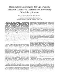
In Appendix D, we prove that this suboptimal policy satisfies the collision probability constraint. Also, in Section V, it is shown by using simulations that the suboptimal policy achieves a near-optimal performance. In Fig. 5, we summarize the operation of the channel access algorithm when the suboptimal policy is applied. V. N UMERICAL R ESULTS We first evaluate the performances of the channel learning and the channel access algorithms separately, and then study the benefit of the combined use of both algorithms. The simulation parameters are as follows: bandwidth of a frequency channel (W ) is 10 MHz; length of a frame is 200 ms; length of a slot (T ) is 20 µs. There are 1000 and 9000 slots in a channel learning subframe and in a channel access subframe, respectively. The threshold for energy detection (δ) is set to 1.16. The set of possible channel usage patterns is given as

k

0 .8

k

k

0 .7

k

^ k

^

-1

^ k -2

0 .6 -3 0 .5 0 .4

-4

0 .3

S N R (d B )

S ta te tra n s itio n ra te s (k H z )

where η(π; a, o) := (ηi,j (π; a, o))(i,j)∈S . The optimal policy β ∗ is a policy such that βn∗ for each n maps a belief vector to a maximizing argument in (20) and (21). Although we can calculate the optimal policy from (20) and (21), the complexity of the dynamic programming in an uncountable set can be prohibitive [31]. Moreover, we should also find the Lagrange multiplier ν that makes the collision probability constraint in (14) satisfied, which requires a high complexity iterative algorithm such as the subgradient method. To overcome this difficulty, we suggest a simple stationary suboptimal policy that exhibits a near-optimal performance in terms of channel utilization while restricting the collision probability within the collision probability limit Clim . The suboptimal policy is ( 1, 1 − π0,0 ≤ Clim sub βn (π) = ∀n = 1, . . . , NA . (22) 0, otherwise

-5 0 .2 -6 0 .1 0 .0

-7 0

5 0 0

1 0 0 0

1 5 0 0

2 0 0 0

2 5 0 0

3 0 0 0

3 5 0 0

4 0 0 0

F ra m e

Fig. 6.

Estimates of the channel usage pattern over frames.

U = {(λ, µ, γ)|λ ≤ 1 kHz, µ ≤ 1 kHz, ρ ≥ −10 dB}. We use the recursive algorithm for estimating the channel usage pattern. We use a constant step size, σk = 10−5 , for the recursive algorithm. We assume that the SU does not switch the frequency channel during simulation time. Fig. 6 demonstrates how well the channel learning algorithm estimates the time-varying channel usage pattern. The channel usage pattern changes in frames 1000, 2000, and 3000. In this figure, we can see that the estimate fluctuates around the real channel usage pattern due to the constant step size. Nonetheless, the channel learning algorithm well tracks the variations of the channel usage pattern. Note that the speed and the accuracy of convergence can be controlled by adjusting the step size σk . We evaluate the performance of the channel access algo-

10

1

U tiliz a tio n a n d c o llis io n p ro b a b ility

U tiliz a tio n a n d c o llis io n p ro b a b ility

1

0 .1

0 .0 1

C o llis io n U tiliz a tio C o llis io n U tiliz a tio C o llis io n

1 E -3

p ro b a b ility lim n , = = 0 .2 P r o b ., = = n , = 0 .2 k H z P ro b ., = 0 .2

0 .0 1

it k H z , 0 .2 k , = k H z ,

S N R = -3 H z , S N R 0 .1 k H z , = 0 .1 k

d B = -3 d B S N R = -5 d B H z , S N R = -5 d B

0 .0 4

0 .0 7

0 .1

0 .0 1

P ro P ro P ro P ro

0 .1

p o s p o s p o s p o s

e d w e d w e d w e d w

ith ith /o /o

le a rn in g , u tiliz a tio n le a rn in g , c o llis io n p ro b . le a rn in g , u tiliz a tio n le a rn in g , c o llis io n p ro b .

1 E -3

C o llis io n p ro b a b ility lim it

1 0 0

5 0 0

1 0 0 0

1 5 0 0

2 0 0 0

2 5 0 0

3 0 0 0

3 5 0 0

4 0 0 0

F ra m e

Fig. 7. Variations in utilization and collision probability with collision probability limit for the proposed channel access algorithm. Fig. 9. Time variation of utilization and collision probability for the proposed schemes with and without the channel learning algorithm. The utilization and collision probability are time-averaged over every 100 frames. 0 .5

0 .4

1 .0

P ro p o s e d w ith le a rn in g P ro p o s e d w /o le a rn in g H e u ris tic

0 .9 0 .8 0 .7 0 .2

P ro p o s P ro p o s H e u ris P ro p o s P ro p o s H e u ris

0 .1

0 .0 0 .0 1

e d , e d , tic , e d , e d , tic ,

s u b o p tim o p tim a l, = = 0 s u b o p tim o p tim a l, = 0 .2 k 0 .1

a l, = = = .2 k H z a l, = = 0 .2 H z , =

C o llis io n p ro b a b ility

0 .6

= 0 .2 k H z

c d f

U tiliz a tio n

0 .3

0 .2 k H z 0 .2 k H z , = 0 .1 k H z k H z , = 0 .1 k H z 0 .1 k H z

0 .5

U tiliz a tio n

0 .4 0 .3 0 .5

C o llis io n P ro b a b ility

0 .2 0 .1 0 .0 0 .0 0 3

Fig. 8. Performance comparison of the proposed channel access algorithms with suboptimal and optimal policies, and the heuristic channel access algorithm in terms of utilization and collision probability. The SNR of a PU signal is set to -4 dB.

rithm in Figs. 7 and 8. For these figures, we assume that the channel usage pattern remains the same over time and is known to the SU so that we can focus on the performance of the channel access algorithm. Fig. 7 shows the utilization and the collision probability for the proposed channel access algorithm with the suboptimal policy as function of the collision probability limit. We can see in the figure that the utilization converges to the probability that a slot is not occupied by the PU as the collision probability increases. This figure shows that the collision probability does not exceed the collision probability limit, regardless of the channel usage pattern. By lowering the collision probability limit, we can decrease the collision probability at the cost of the utilization. Fig. 8 compares the performances of the proposed channel access algorithm (with suboptimal and optimal policies) and the performances of the heuristic channel access algorithm. We compare the proposed algorithm with a simple listenbefore-talk heuristic algorithm. If the sensing result in slot (n − 1) indicates that the channel is inactive, the heuristic

0 .0 1

0 .1

1

U tiliz a tio n a n d c o llis io n p ro b a b ility

Fig. 10. Cumulative density functions of utilization and collision probability when the proposed schemes with and without the channel learning algorithm and the heuristic channel access algorithm are used.

algorithm transmits data for τ consecutive slots from slot n until it performs another energy detection. Thus, τ balances the tradeoff between the utilization and the collision probability for the heuristic algorithm. The graphs are plotted by varying Clim for the proposed algorithm with the suboptimal policy, ν and Clim for the proposed algorithm with the optimal policy, and τ for the heuristic algorithm. In this figure, we can see that the proposed algorithm with the suboptimal policy exhibits performance very close to the optimal one. Therefore, we can say that the suboptimal policy is a very useful lowcomplexity alternative to the optimal policy, accomplishing a near-optimal performance as well as effectively limiting the collision probability. We also observe that the proposed algorithm outperforms the heuristic algorithm. The proposed algorithm can achieve very low collision probability owing to its resilience to sensing errors, whereas the heuristic algorithm cannot.

11

In Figs. 9-10, we consider the channel learning algorithm as well as the channel access algorithm to investigate the impact of channel learning on the system performance. Fig. 9 shows the time variation of the utilization and the collision probability of the proposed schemes with and without the channel learning algorithm. Since the proposed scheme with learning consumes additional NL slots for channel learning, for fairness in comparison, we multiply NA /(NL + NA ) to the utilization of the proposed scheme with learning. For both the schemes, the collision probability limit, Clim , is set to 0.03. While the proposed scheme with learning utilizes the channel usage pattern estimated by the channel learning algorithm to adjust the parameters of the channel access algorithm, the proposed scheme without learning just assumes that λ = µ = 0.3 kHz and γ = −3 dB. The channel usage pattern uk varies over time as follows: (0.4 kHz, 0.4 kHz, −3 dB) for k = 1, . . . , 1000, (0.6 kHz, 0.2 kHz, −5 dB) for k = 1001, . . . , 2000, (0.1 kHz, 0.6 kHz, −2 dB) for k = 2001, . . . , 3000, and (0.4 kHz, 0.2 kHz, −6 dB) for k = 3001, . . . , 4000. From Fig. 9, we observe that the proposed scheme without learning violates the collision probability limit and imposes excessive interference to PU traffic, when the channel usage pattern is unfavorable. On the other hand, for the proposed scheme with learning, the collision probability remains below the collision probability limit, irrespective of how the channel usage pattern varies. This is due to the fact that the scheme with learning is able to adapt its parameters to the varying channel usage pattern. In Fig. 10, we compare the cumulative distribution functions (cdf’s) of the utilization and the collision probability when the proposed schemes with and without learning and the heuristic channel access algorithm are used. We estimate the utilization and the collision probability in each frame and calculate the corresponding cumulative distribution functions. The channel usage pattern randomly changes over frames. The duration between consecutive changes in the channel usage pattern follows a geometric distribution with an average of 1000 frames. The state transition rates λ and µ are selected from a uniform distribution over [0.1 kHz, 1 kHz], and the SNR of PU signals is uniformly distributed over [−6 dB, −3 dB]. The collision probability limit is set to 0.03. The proposed scheme without learning assumes that λ = µ = 0.8 kHz and γ = −6 dB. For the heuristic algorithm, we set τ = 1 to reduce the collision probability of the heuristic algorithm as much as possible. From Fig. 10, we observe that the collision probability limit is frequently violated by the proposed scheme without learning and the heuristic algorithm, while the proposed scheme with learning well keeps the collision probability below the limit. The proportions of the frames in which the collision probability exceeds the limit are 0.07, 0.08, and 0.61 for the proposed schemes with and without learning, and the heuristic algorithm, respectively. From this figure, we can conclude that the proposed scheme with learning can effectively maintain the collision probability under the target limit. While keeping the collision probability, the proposed scheme with learning also has the average utilization (i.e., 0.31) considerably higher than the proposed scheme without learning (i.e., 0.18) and the heuristic algorithm (i.e., 0.24).

VI. C ONCLUSION We have proposed a channel sensing and channel access scheme that opportunistically exploits frequency channels occupied by a data-centric primary user network. The proposed scheme repeats a learning and access cycle, driven by the channel learning and the channel access algorithms. To make the scheme robust to high sensing error probability, we have applied the hidden Markov model (HMM) and partially observable Markov decision process (POMDP) frameworks to the channel learning and the channel access algorithms, respectively. The simulation results have shown that, by adapting to varying channel usage pattern, the proposed scheme provides efficient access to spectrum opportunities while constraining the interference to the primary users below the target limit. The proposed scheme outperforms a heuristic algorithm without any learning functionality. Extension of the scheme to a distributed multiuser scenario will be considered in our future work. A PPENDIX A. Proof of the Condition for Equivalence of Two AMPs ˜ be the channel usage patterns corresponding Let u and u ˜ respectively. The probability of to the AMPs with h and h, an observation sequence x = {x1 , . . . , xN } given the channel usage pattern u can be rewritten as Pr[o = x|u] = 1T · IxN h · IxN −1 h · · · Ix2 h · Ix1 π = 1T hxN hxN −1 · · · hx2 π x1

(23)

where π := (π 0 , π 1 )T is a column vector of the initial state distribution in which π 0 and π 1 are 2-by-1 column vectors, I0 := diag(1, 1, 0, 0), and I1 := diag(0, 0, 1, 1). ˜ 0 τ = 0. We first consider the case that 1T h0 τ = 0 and 1T h T T T˜ In this case, we have 1 hx = 1 yx and 1 hx = 1T y˜x for x = 0, 1 and some real values y0 , y1 , y˜0 , and y˜1 . Then, we have Pr[o = x|u] = yxN yxN −1 · · · yx2 yx1 and Pr[o = x|˜ u] = ˜ are equivalent y˜xN y˜xN −1 · · · y˜x2 y˜x1 . The AMPs with h and h if and only if yxN yxN −1 · · · yx2 yx1 and y˜xN y˜xN −1 · · · y˜x2 y˜x1 are the same for all observation sequences x. This condition is satisfied only when yx = y˜x for x = 0, 1. Therefore, we ˜ 0 should be satisfied for the can conclude that 1T h0 = 1T h equivalence of two AMPs. ˜ 0 τ 6= 0. We now consider the case that 1T h0 τ 6= 0 or 1T h The proof for this case is based on the result in [28]. Let V denote the null space defined by V := {π|1T · IxN h · IxN −1 h · · · Ix2 h · Ix1 π = 0 ∀x}. (24) The vector in the null space should satisfy 1T π 0 = 0, 1T h0 π 0 = 0, 1T π 1 = 0, and 1T h0 π 1 = 0. If 1T h0 τ 6= 0, the only vector satisfying the condition is the zero vector. In ˜ are equivalent [28], it is shown that the AMPs with h and h ˜ if and only if h and h are similar via some block diagonal matrix preserving the probability, on the quotient space where the null space is factored out. Since the null space has zero dimension in this case, the AMPs are equivalent if and only if there exists a 2-by-2 matrix X such that ˜ 0 X, and Xh1 = h ˜ 1 X. 1T X = 1T , Xh0 = h (25)

12

B. Proof of the Condition for Identifiability of an AMP T

If 1 h0 τ = 0, there can be an infinite number of AMPs ˜ 6= h that satisfies with the transition probability matrix h T˜ T 1 h0 = 1 h0 . Since these AMPs are equivalent to the AMP with h from Theorem 1, it should be satisfied that 1T h0 τ 6= 0 for the AMP to be identifiable. ˜ that is equivalent Suppose that there exists an AMP with h to the AMP with h when 1T h0 τ 6= 0. Then, from Theorem 1, ˜ 0 X, and there exists X 6= I such that 1T X = 1T , Xh0 = h ˜ 1 X. We can calculate h ˜ 0 = Xh0 X−1 and h ˜1 = Xh1 = h Xh1 X−1 . These matrices should satisfy, for some r˜i,j and γ˜ ,   γ )) ˜ 0 = r˜0,0 (1 − D(0)) r˜1,0 (1 − Υ(˜ h (26) r˜0,1 (1 − Υ(˜ γ )) r˜1,1 (1 − D(˜ γ )) and  r˜ D(0) ˜ h1 = 0,0 r˜0,1 Υ(˜ γ)

 r˜1,0 Υ(˜ γ) . r˜1,1 D(˜ γ)

(27)

Therefore, we have 1T X = 1T and F(˜ γ ) ◦ (Xh0 X−1 ) = G(˜ γ ) ◦ (Xh1 X−1 ). (28) If there is no X 6= I and γ˜ ≥ 0 satisfying the above condition, we can say that there is no AMP equivalent to the AMP with h. C. Calculation of the Gradient of Ξ(o; u) We calculate the partial derivatives of Ξ(o; u) with respect to λ, µ, and γ. To do this, we first define φ(o; u) := Pr[o|u]. Recall that αn is the PU activity at time t = (n − 1)T when t = 0 at the start of the channel learning subframe. Let us define α := (α1 , . . . , αNL +1 ). Then, φ(o; u) can be rewritten as the sum of the probabilities Pr[o, α|u]’s for all possible P α’s, that is, φ(o; u) = α κ(o, α; u), where κ(o, α; u) = Pr[o, α|u] = bα1

NL Y

rαn ,αn+1 ·

qαonn ,αn+1 .

n=1

(29) In the above equation, we define bi := Pr[α1 = i] and ri,j := Pr[αn+1 = j|αn = i]. Then, we have b0 = µ/(λ + µ), b1 = λ/(λ + µ), r0,0 = e−λT , r0,1 = 1 − e−λT , r1,0 = 1 − e−µT , and r1,1 = e−µT . In addition, using the definition of Υ(γ), 1 0 0 = 1 − D(0), q0,0 = D(0), q0,1 = 1 − Υ(γ), we have q0,0 1 0 1 0 q0,1 = Υ(γ), q1,0 = 1 − Υ(γ), q1,0 = Υ(γ), q1,1 = 1 − D(γ), 1 and q1,1 = D(γ). First, we calculate the derivative of κ(o, α; u) with respect to an arbitrary variable x. That is, X ∂bi 1 ∂κ (o, α; u) = · · 1α1 =i Pr[o, α|u] ∂x ∂x bi i∈{0,1}

+

NL X ∂ri,j 1 X · · 1s =(i,j) Pr[o, α|u] ∂x ri,j n=1 n

(i,j)∈S

+

where S is the state space, O is the observation space, and 1X is a function that is 1 if X is true; and 0 otherwise. Now, we calculate ∂Ξ/∂x as X ∂κ(o, α; u) 1 ∂φ(o; u) 1 ∂Ξ (o; u) = · = · ∂x φ(o; u) ∂x φ(o; u) α ∂x  X 1 ∂bi 1 = · · · ωi (o; u) φ(o; u) ∂x bi i∈{0,1}

X ∂ri,j 1 + · · χi,j (o; u) ∂x ri,j (i,j)∈S

 m X X ∂qi,j 1 m (31) + · m · ψi,j (o; u) ∂x qi,j (i,j)∈S m∈V

where we define i, o|u], PNL ωi (o; u) := Pr[α1 = m χ n=1 Pr[sn = (i, j), o|u], and ψi,j (o; u) := Pi,j (o; u) := n|on =m Pr[sn = (i, j), o|u]. From this equation, we can calculate ∂Ξ/∂λ, ∂Ξ/∂µ, and ∂Ξ/∂γ. For example, we can derive ∂Ξ/∂λ as  1 ∂b0 1 ∂b1 1 ∂Ξ (o; u) = · · · · ω0 (o; u) + · ω1 (o; u) ∂λ φ(o; u) ∂λ b0 ∂λ b1 1 ∂r0,0 · · χ0,0 (o; u) + ∂λ r0,0  1 ∂r0,1 · + · χ0,1 (o; u) ∂λ r0,1  1 µ · ω1 (o; u) ω0 (o; u) = · − φ(o; u) λ(λ + µ) λ+µ  T · χ0,1 (o; u) − T · χ0,0 (o; u) . (32) + eλT − 1 We can also calculate ∂Ξ/∂µ and ∂Ξ/∂γ in a similar way. D. The Suboptimal Policy Satisfies the Collision Probability Constraint Proof: We prove that collision probability does not exceed the collision probability limit, i.e., C ≤ Clim , when the sub suboptimal policy β sub = (β1sub , . . . , βN ) is applied. Provided A sub that β is used, we can rewrite the collision probability as PNA n=1 Pr[sn 6= (0, 0), an = 1] C = PNA n=1 Pr[an = 1] PNA P n=1 Γn Pr[sn 6= (0, 0), 1 − π0,0 ≤ Clim |Γn ] · Pr[Γn ] = PNA P n=1 Γn Pr[1 − π0,0 ≤ Clim |Γn ] · Pr[Γn ] (33) where Γn := {π 1 , a1 , . . . , an−1 , o1 , . . . , on−1 }. Since π0,0 only depends on Γn , the value of Pr[1 − π0,0 ≤ Clim |Γn ] in the denominator in (33) is one if 1 − π0,0 ≤ Clim ; and zero, otherwise. Also, Pr[sn 6= (0, 0), 1 − π0,0 ≤ Clim |Γn ] in the numerator in (33) is calculated as

NL m X X ∂qi,j 1 X · m · 1s =(i,j),on =m Pr[o, α|u] ∂x qi,j n=1 n

(i,j)∈S m∈O

(30)

Pr[sn 6= (0, 0), 1 − π0,0 ≤ Clim |Γn ] = ( 1 − π0,0 , if 1 − π0,0 ≤ Clim 0, otherwise.

(34)

13

Therefore, the inequality Pr[sn 6= (0, 0), 1−π0,0 ≤ Clim |Γn ] ≤ [22] Clim · Pr[1 − π0,0 ≤ Clim |Γn ] is satisfied. Applying this [23] inequality to (33), we can conclude that PNA P [24] Γn Clim · Pr[1 − π0,0 ≤ Clim |Γn ] · Pr[Γn ] = Clim . C ≤ n=1 PNA P n=1 Γn Pr[1 − π0,0 ≤ Clim |Γn ] · Pr[Γn ] [25]

R EFERENCES [1] S. Geirhofer, L. Tong, and B. M. Sadler, “A measurement-based model for dynamic spectrum access in WLAN channels,” in Proc. IEEE MILCOM’06, Washington, D.C., Oct. 2006. [2] S. Geirhofer, L. Tong, and B. M. Sadler, “Dynamic spectrum access in the time domain: Modeling and exploiting white space,” IEEE Commun. Mag., vol. 45, no. 5, pp. 66–72, May 2007. [3] S. D. Jones, E. Jung, X. Liu, N. Merheb, and I. J. Wang, “Characterization of spectrum activities in the U.S. public safety band for opportunistic spectrum access,” in Proc. IEEE DySPAN’07, Dublin, Ireland, Apr. 2007. [4] M. Wellens, J. Riihij¨arvi, and P. M¨ah¨onen, “Empirical time and frequency domain models of spectrum use,” Physical Communication (Elsevier), vol. 2, no. 1–2, pp. 10–32, Mar. 2009. [5] M. Wellens and P. M¨ah¨onen, “Lessons learned from an extensive spectrum occupancy measurement campaign and a stochastic duty cycle model,” in Proc. TridentCom09, Washington, D.C., Apr. 2009. [6] D. Willkomm, S. Machiraju, J. Bolot, and A. Wolisz, “Primary user behavior in cellular networks and implications for dynamic spectrum access,” IEEE Commun. Mag., vol. 47, no. 3, pp. 88–95, Mar. 2009. [7] Q. Zhao, L. Tong, A. Swami, and Y. Chen, “Decentralized cognitive MAC for opportunistic spectrum access in ad hoc networks: A POMDP framework,” IEEE J. Sel. Areas Commun., vol. 25, no. 3, pp. 589–600, Apr. 2007. [8] Q. Zhao, B. Krishnamachari, and K. Liu, “On myopic sensing for multi-channel opportunistic access: Structure, optimality, and performance,” IEEE Trans. Wireless Commun., vol. 7, no. 12, pp. 5431–5440, Dec. 2008. [9] Q. Zhao, S. Geirhofer, L. Tong, and B. M. Sadler, “Opportunistic spectrum access via periodic channel sensing,” IEEE Trans. Signal Process., vol. 56, no. 2, pp. 785–796, Feb. 2008. [10] H. Su and X. Zhang, “Cross-layer based opportunistic MAC protocols for QoS provisionings over cognitive radio wireless networks,” IEEE J. Sel. Areas Commun, vol. 26, no. 1, pp. 118–129, Jan. 2008. [11] S. Geirhofer, L. Tong, and B. M. Sadler, “Cognitive medium access: Constraining interference based on experimental models,” IEEE J. Sel. Areas Commun, vol. 26, no. 1, pp. 95–105, Jan. 2008. [12] S. Huang, X. Liu, and Z. Ding, “Opportunistic spectrum access in cognitive radio networks,” in Proc. IEEE INFOCOM’08, Phoenix, AJ, Apr. 2008. [13] R. Urgaonkar and M. J. Neely, “Opportunistic scheduling with reliability guarantees in cognitive radio networks,” IEEE Trans. Mobile Comput., vol. 8, no. 6, pp. 766–777, Jun. 2009. [14] Y.-C. Liang, Y. Zeng, E. C. Y. Peh, and A. T. Hoang, “Sensingthroughput tradeoff for cognitive radio networks,” IEEE Trans. Wireless Commun., vol. 7, no. 4, pp. 1326–1337, Apr. 2008. [15] H. Kim and K. G. Shin, “Efficient discovery of spectrum opportunities with MAC-layer sensing in cognitive radio networks,” IEEE Trans. Mobile Comput., vol. 7, no. 5, pp. 533–545, May 2008. [16] L. Lai, H. El Gamal, H. Jiang, and H. V. Poor, “Cognitive medium access: Exploration, exploitation and competition,” IEEE/ACM Trans. Netw., submitted for publication. [Online]. Available: http://www.ece.osu.edu/∼helgamal/ [17] H. Jiang, L. Lai, R. Fan, and H. V. Poor, “Optimal selection of channel sensing order in cognitive radio,” IEEE Trans. Wireless Commun., vol. 8, no. 1, pp. 297–307, Jan. 2009. [18] R. Fan and H. Jiang, “Channel sensing-order setting in cognitive radio networks: A two-user case,” IEEE Trans. Veh. Technol., vol. 58, no. 9, pp. 4997–5008, Nov. 2009. [19] L. R. Rabiner, “A tutorial on hidden Markov models and selected applications in speech recognition,” Proceedings of the IEEE, vol. 77, no. 2, pp. 257–286, Feb. 1989. [20] T. Ryd´en, “On recursive estimation for hidden Markov models,” Stochastic Processes and their Applications, vol. 66, no. 1, pp. 79–96, Feb. 1997. [21] S. Huang, X. Liu, and Z. Ding, “Optimal transmission strategies for dynamic spectrum access in cognitive radio networks,” IEEE Trans. Mobile Comput., vol. 8, no. 12, pp. 1636–1648, Dec. 2009.

[26] [27] [28]

[29] [30] [31]

T. Clancy and B. Walker, “Predictive dynamic spectrum access,” in Proc. SDR Forum Technical Conference, Orlando, FL, Nov. 2006. I. A. Akbar and W. H. Tranter, “Dynamic spectrum allocation in cognitive radio using hidden markov models: Poisson distributed case,” in Proc. SoutheastCon 2007, Richmond, VA, Mar. 2007. G. E. Monahan, “A survey of partially observable Markov decision processes: Theory, models, and algorithms,” Management Science, vol. 28, no. 1, pp. 1–16, Jan. 1982. J. Jia, Q. Zhang, and X. Shen, “HC-MAC: A hardware-constrained cognitive MAC for efficient spectrum management,” IEEE J. Sel. Areas Commun, vol. 26, no. 1, pp. 106–117, Jan. 2008. H. Urkowitz, “Energy detection of unknown deterministic signals,” Proceedings of the IEEE, vol. 55, no. 4, pp. 523-531, Apr. 1967. Y. Ephraim and N. Merhav, “Hidden Markov processes,” IEEE Trans. Inf. Theory, vol. 48, no. 6, pp. 1518–1569, Jun. 2002. H. Ito, S.-I. Amari, and K. Kobayashi. “Identifiability of hidden Markov information sources and their minimum degrees of freedom,” IEEE Transactions on Information Theory, vol. 38, no. 2, pp. 324–333, Mar. 1992. L. E. Baum and T. Petrie, “Statistical inference for probabilistic functions of finite state Markov chains,” The Annals of Mathematical Statistics, vol. 37, no. 6, pp. 1554–1563, Dec. 1966. K. W. Choi, “Adaptive sensing technique to maximize spectrum utilization in cognitive radio,” IEEE Trans. Veh. Technol., vol. 59, no. 2, pp. 992–998, Feb. 2010. W. S. Lovejoy, “A survey of algorithmic methods for partially observable Markov decision processes,” Annals of Operations Research, vol. 28, no. 1, pp. 47–66, Dec. 1991.

Kae Won Choi received the B.S. degree in civil, urban, and geosystem engineering in 2001, and the M.S. and Ph.D. degrees in electrical engineering and computer science in 2003 and 2007, respectively, all from Seoul National University, Seoul, Korea. From 2008 to 2009, he was with Telecommunication Business of Samsung Electronics Co., Ltd., Korea. From 2009 to 2010, he was a postdoctoral researcher in the Department of Electrical and Computer Engineering, University of Manitoba, Winnipeg, MB, Canada. In 2010, he joined the faculty at Seoul National University of Science and Technology, Korea, where he is currently an assistant professor in the Department of Computer Science. His research interests include cognitive radio, wireless network optimization, radio resource management, and mobile cloud computing.

Ekram Hossain (S’98-M’01-SM’06) is a full Professor in the Department of Electrical and Computer Engineering at University of Manitoba, Winnipeg, Canada. He received his Ph.D. in Electrical Engineering from University of Victoria, Canada, in 2001. Dr. Hossain’s research interests include design, analysis, and optimization of wireless/mobile communications networks and cognitive radio systems (http://www.ee.umanitoba.ca/∼ekram). He serves as the Area Editor for the IEEE Transactions on Wireless Communications in the area of “Resource Management and Multiple Access”, an Editor for the IEEE Transactions on Mobile Computing, the IEEE Communications Surveys and Tutorials, and IEEE Wireless Communications. Dr. Hossain has several research awards to his credit which include the University of Manitoba Merit Award in 2010 (for Research and Scholarly Activities) and the 2011 IEEE Communications Society Fred Ellersick Prize Paper Award. He is a registered Professional Engineer in the province of Manitoba, Canada.