NOTATION

Closed-Form Posterior Cram´er-Rao Bounds for Bearings-Only Tracking

LP(C) MP(C) BOT Xt Yt ny 3

(BOT) for a single object, which belongs to the general class

Idn 0n£m − X¤ kXk2Q ± ¢ r det(X) pdf

of nonlinear filtering problems. Recently, algorithms based on

A

T. BREHARD J.-P. LE CADRE IRISA/CNRS France

We address the classical bearings-only tracking problem

sequential Monte-Carlo methods (particle filtering) have been proposed. As far as performance analysis is concerned, the posterior Crame´ r-Rao bound (PCRB) provides a lower bound on the mean square error. Classically, under a technical assumption

H Q

named “asymptotic unbiasedness assumption,” the PCRB is given by the inverse Fisher information matrix (FIM). The latter is computed using Tichavsky´ ’s recursive formula via Monte-Carlo methods. Two major problems are studied here. First, we show that the asymptotic unbiasedness assumption can be replaced by an assumption which is more meaningful. Second, an exact algorithm to compute the PCRB is derived via Tichavsky´ ’s recursive formula without using Monte-Carlo methods. This result is based on a new coordinate system named logarithmic polar coordinate (LPC) system. Simulation results illustrate that PCRB can now be computed accurately and quickly, making it suitable for sensor management applications.

Manuscript received December 20, 2003; revised March 4 and December 9, 2005; released for publication February 25, 2006. IEEE Log No. T-AES/42/4/890174. Refereeing of this contribution was handled by B. La Scala. Authors’ address: IRISA/CNRS, Campus de Beaulieu, 35042 Rennes Cedex, France. E-mail: ([email protected]). c 2006 IEEE 0018-9251/06/$17.00 ° 1198

Logarithmic polar coordinates Modified polar coordinates Bearings-only tracking Target state in Cartesian coordinate system Target state in LPC system Size of target state (ny = 4) Inequality R3S means that R ¡ S is positive semi-definite matrix n £ n identity matrix n £ m matrix composed of zero element Kronecker product Denotes transpose of matrix X = EfX ¤ Q¡1 Xg where X is column vector Dirac delta function Laplacian operator Gradient operator Determinant of matrix X Probability density function · ¸ 0 1 = Id4 + ±t B with B = − Id2 0 0 μ ¶ ± = t − Id2 1 μ ¶ ®3 ®2 = § − Id2 with § = . ®2 ®1

I. INTRODUCTION In many applications (submarine tracking, aircraft surveillance), a bearings-only sensor is used to collect observations about target trajectory. This problem of tracking has been of interest for the past thirty years. The aim of bearings-only tracking (BOT) is to determine the target trajectory using noise-corrupted bearing measurements from a single observer. Target motion is classically described by a diffusion model1 so that the filtering problem is composed of two stochastic equations. The first one represents the temporal evolution of the target state (position and velocity) called state equation. The second one links the bearing measurement to the target state at time t (measurement equation). One of the characteristics of the problem is the nonlinearity of the measurement equation so that the classical Kalman filter is not convenient in this case. We can find in literature two kinds of solutions to this problem. The first one, proposed by Lindgren and Gong in [2], consists of deriving a pseudolinear measurement equation. Then, a Kalman filter can be used to solve the problem. The stochastic stability analysis of the estimates had been addressed by Song and Speyer in [3]. However, Aidala and Nardone show in [4] that this approach produces bias range estimates which can be reduced if the observer 1 See

[1] for an exhaustive review on dynamic models.

IEEE TRANSACTIONS ON AEROSPACE AND ELECTRONIC SYSTEMS VOL. 42, NO. 4

Authorized licensed use limited to: UR Rennes. Downloaded on July 10, 2009 at 11:18 from IEEE Xplore. Restrictions apply.

OCTOBER 2006

executes a maneuver. Consequently, bias range can be estimated as soon as it becomes observable [5]. A second idea consists of using the extended Kalman filter (EKF) in a Cartesian coordinate system to solve the problem. However, simulations show that this algorithm is often divergent due to the weak observability of range [6—8]. To remedy this problem, Aidala and Hammel in [9] proposed an EKF using another system named modified polar coordinate (MPC) system whose one salient feature is that range is not coupled with the observable components. This constitutes a neat improvement. Another solution proposed by Peach in [10] is a range-parametrized EKF, in which a number of EKF trackers parametrized by range run in parallel. Recently, particle filtering algorithms have been proposed in this context [11—13]. In [14], Arulampalam and Ristic compare the particle filter with the range-parametrized and EKF in MPC system; while a comprehensive overview of the state of art can be found in [15]. As far as performance analysis is concerned, the posterior Crame´ r-Rao bound (PCRB) proposed in [16] is widely used to assess the performance of filtering algorithms, by the tracking community [17—20] and in particular in the bearings-only context [15, 21, 22]. The PCRB gives a lower bound for the error covariance matrix (ECM). More precisely, under a technical assumption, the PCRB is the inverse of the Fisher information matrix (FIM). A seminal contribution on performance analysis is the paper from Tichavsky´ , et al. [23]. Here, the authors noticed that only the right lower block of the FIM inverse was of interest for investigating tracking performance. This was the key idea for deriving a practical updating formula for the PCRB. Recently, PCRB has been used for various sensor management problems like automating the deployment of sensors in [24] or determining the optimal sensor trajectory in the bearings-only context in [25]. Moreover, PCRB can be used to schedule active measurements in a system involving active and passive subsystems. This application is addressed in the simulation section. However, some problems remain to be solved. In this paper, two major issues of the PCRB are addressed. First, under a technical assumption named “asymptotic unbiasedness assumption,” the PCRB is the FIM inverse. However, the validity of this assumption has not been thoroughly investigated in the BOT context yet. Here, our approach consists of deriving the PCRB in an original coordinate system named logarithmic polar coordinate (LPC) system. Using this coordinate system, it is shown that the asymptotic unbiasedness assumption can be replaced with another one, more meaningful in the BOT context. Second, Tichavsky´ ’s recursive formula is a powerful result to compute the right lower block of

the FIM inverse. However, complex integrals without any closed forms are involved in this recursion. So, these complex integrals must be approximated via Monte-Carlo methods. This approach is quite feasible but induces high computation requirements which highly reduces its suitability for complex problems like sensor management. For instance, the aim of active measurement scheduling consists in optimizing the time distribution of range measurements to obtain an accurate target state estimate. It implies to perform Monte-Carlo evaluations of the PCRB for each policy, which would rapidly become infeasible. To avoid this problem, Ristic, et al. in [15] assume that the target process noise is zero. In the general case, we show that the complex integrals required for calculating the PCRB admit closed-form expressions if the PCRB is derived in the LPC system. Remarkably, though this coordinate system is only a slight modification of the MPC [9], it allows instrumental simplifications in the calculation of the elementary terms of the PCRB recursion. Applications to active measurement scheduling is briefly considered in a simulation framework. In Section II, the BOT problem is presented in the Cartesian coordinate system and then in the LPC system. This original coordinate system is the key point to derive a closed form for the PCRB. In Section III, the classical PCRB is presented. A close examination of the asymptotic unbiasedness assumption is achieved so as to prove the validity of the “usual” PCRB, as given by the FIM inverse. We study this assumption and derive a more meaningful condition. In particular, conditions ensuring its validity are examined in the BOT context. Calculation of closed-form expressions of the right lower block of the FIM inverse via Tichavsky´ ’s recursive formula is addressed in Section IV, in the LPC setting. Then, the closed-form PCRB is investigated for scheduling active measurements in Section V. In Section VI, simulation results present a comparison between the closed-form PCRB and the classical one (i.e., where the terms involved in Tichavsky´ ’s formula are approximated by Monte-Carlo methods). Finally, the closed-form PCRB is used for investigating scheduling of passive and active measurements. II.

FROM CARTESIAN TO LPC SYSTEM

A. Cartesian Framework for BOT Historically, BOT is presented in the Cartesian system. Let us define target state at time t: Xt = [rx (t) ry (t) vx (t) vy (t)]¤

(1)

made of target relative velocity and position in the x-y plane. It is assumed that the target follows a nearly constant-velocity model. The discretized state

´ BREHARD & LE CADRE: CLOSED-FORM POSTERIOR CRAMER-RAO BOUNDS FOR BEARINGS-ONLY TRACKING

Authorized licensed use limited to: UR Rennes. Downloaded on July 10, 2009 at 11:18 from IEEE Xplore. Restrictions apply.

1199

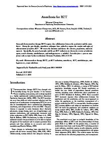
Fig. 1. Two examples of pdf of Zt given Xt . (a) If Zt is far from the bounds. (b) If Zt is close to ¼=2.

equation2 is given by Xt+1 = AXt + Ut + ¾Wt

(2)

where Wt » N (0, Q) A = Id4 + ±t B Q = § − Id2

with B = with § =

·

·

0 1 0 0

¸

®3

®2

®2

®1

− Id2 ¸

:

and ±t is the elementary time period and ¡Ut is the known difference between observer velocity at time t + 1 and t. The state covariance ¾ is unknown. However we assume classically that ¾ < ¾max , so that we use in practice the following equation: Xt+1 = AXt + Ut + ¾max Wt :

(3)

Otherwise, we note Zt the bearing measurement received at time t. The target state is related to this measurement through the following equation: μ ¶ X Zt = arctan

rx (t) ry (t)

+ Vt +

k2Z

|

N (0, ¾¯2 )

k¼1¡¼=2
{z (?)

}

(4)

1200

Thus, the target state at time t is defined by (5), where ¯t and rt are the relative bearing and target range. We propose in the following section a slight modification of the MPC system, named the LPC system. The only difference is that the second component is not 1=rt but ln(rt ). Even if this tiny difference appears very minor, it will be shown that it is instrumental for deriving a closed form of the PCRB. Let us now derive BOT equations given by (3) and (4) in the LPC framework.

¾¯2

where Vt » and is known. Let us notice that the term (?) is usually omitted. However, it is necessary to consider that measurement Zt is restricted to a part of the space. This is the case if symmetry of the receiver (e.g. linear array) leads to considering measurements belonging in the interval ] ¡ ¼=2, ¼=2[, so that the additional term (?) in (4) is necessary. Two examples of probability density function (pdf) of Zt given Xt are presented in Fig. 1 to enlighten the importance of the additional term (?). In Fig. 1(b), the bearing measurement is close to ¼=2 so that there is an overlapping phenomena. 2 For

The system (3)—(4) has two components: a linear state equation (3) and a nonlinear measurement equation (4). Particle filter techniques [26, 27] are, thus, particularly appealing. Otherwise, practical implementations of EKF-based algorithms [9, 10] use a specific coordinate system, namely MPC. Indeed, if the target follows a deterministic trajectory (i.e., Wt = 0 8t 2 f0, : : : , Tg in (3)), Nardone and Aidala have demonstrated in [7] that no information on range exists as long as the observer is not maneuvering. So the idea consists of using a coordinate system for which unobservable component (range) is not coupled with the observable part. This is also the motivation of Aidala and Hammel [9] for defining the MPC system: · ¸¤ 1 _ r_t ¯t ¯t : (5) rt rt

a general review of dynamic models for target tracking see [1].

B. LPC Framework for BOT We consider now that the system state Yt is expressed in the LPC system, i.e., Yt = [¯t ½t ¯_ t ½_ t ]¤

(6)

where ½t = ln rt : As between Cartesian and modified polar (MP) system, we do not have a direct bijection between the Cartesian and the LPC system due to arctan function definition. We just have flpc and fclp , respectively LPC-to-Cartesian and Cartesian-to-LPC state mapping

IEEE TRANSACTIONS ON AEROSPACE AND ELECTRONIC SYSTEMS VOL. 42, NO. 4

Authorized licensed use limited to: UR Rennes. Downloaded on July 10, 2009 at 11:18 from IEEE Xplore. Restrictions apply.

OCTOBER 2006

A. Classical PCRB

functions such that ½ c flp (Yt ) if ry (t) > 0 Xt = ¡flpc (Yt ) if ry (t) < 0 2 3 sin ¯t 6 7 cos ¯t 6 7 7 flpc (Yt ) = rt 6 6 ¯_ cos ¯ + ½_ sin ¯ 7 4 t t t t 5 ¡¯_ sin ¯ + ½_ cos ¯ t

t

t

and

(7)

!

x

y

k2Z

(10)

First, let us recall the FIM and bias definitions. 3

DEFINITION 1 (FIM) For the filtering problem given by (9), the FIM, at time t, is denoted J0 : t and defined as J0 : t = EfrY0 : t ln p(Z1 :t , Y0 : t )r¤Y0 : t ln p(Z1 : t , Y0 : t )g (11) (8)

where p(Z1 : t , Y0 : t ) is the joint pdf of Z1 :t and Y0 : t . DEFINITION 2 (Bias) For the filtering problem described by (9), estimation bias related to the estimated trajectory Yˆ0 : t is defined as:

y

Thus, using (7) and (8), the stochastic system given by (3) and (4) becomes ( lp fc (Aflpc (Yt ) + Ut + ¾max Wt ) if ry (t) > 0 Yt+1 = fclp (¡Aflpc (Yt ) + Ut + ¾max Wt ) if ry (t) < 0 X

0:t

ECM0 : t = kYˆ0 : t ¡ Y0 : t k2 :

rx2 (t) + ry2 (t)

Zt = ¯t + Vt +

0:t

Z1 : t . We focus here on the ECM at time t which is ny (t + 1) £ ny (t + 1)-matrix, defined by

rx (t) 7 6 arctan r (t) y 7 6 7 6 ´ ³q 7 6 2 2 6 ln rx (t) + ry (t) 7 7 6 7 Yt = fclp (Xt ) = 6 6 vx (t)ry (t) ¡ vy (t)rx (t) 7 : 7 6 7 6 rx2 (t) + ry2 (t) 7 6 7 6 4 v (t)r (t)) + v (t)r (t) 5 x

Let Y0 : t and Z1 : t be the trajectory and the set of bearing measurements up to time t. They are random vectors of size ny (t + 1) and t, respectively. Let Yˆ be an estimator of Y which is a function of

t

Ã

2

with

(9) k¼1¡¼=2<¯t +Vt +k¼<¼=2 :

Though it seems that the LPC increases the complexity of the BOT problem, it has also the advantage of highlighting the multi-modality associated with the two solutions corresponding to ry (t) > 0 and ry (t) < 0, respectively. III. PCRB FOR STATE ESTIMATION In this section, “usual” PCRB given by the inverse FIM is presented. Notably, in subsection A, we present the proof of this classical result. The role of a technical hypothesis named asymptotic unbiasedness assumption is thus highlighted, especially in the LPC system. Then, we show in subsection B that this hypothesis is not always satisfied in the BOT context and we propose to replace it by an original extension. Finally, it is shown that the usual PCRB as given by FIM inverse is valid if bearing measurements are sufficiently far from ¡¼=2 and ¼=2. Let us remark that the PCRB is not derived in the Cartesian framework for two reasons. First, the asymptotic unbiasedness assumption seems rather difficult to address in this setting. Second, it is shown that a closed form exists in LPC but not in the classical coordinate systems (Cartesian or MPC).

B(Y0 : t ) = EfYˆ0 : t ¡ Y0 : t j Y0 : t g:

(12)

Y0 :t is a ny (t + 1) vector so that B(Y0 : t ) is a ny (t + 1) vector too. The estimator of the trajectory Yˆ is 0:t

unbiased if vector B(Y0 :t ) is almost surely equal to zero. This choice of the bias definition is justified in Appendix A. Proposition 1 ensures that the FIM gives a lower bound for the ECM under a specific assumption called asymptotic unbiasedness assumption. Before introducing this technical assumption let us introduce a notation to simplify the presentation: Notation 1 For a function F : Rd ! Rn , U and U two Rd -vectors such that U = [U1 , : : : , Ud ]¤ and U = [U1 , : : : , Ud ]¤ , we define 2 3 6 lim F(U) = 6 4 U!U

limU1 !U1 (F(U))1

¢¢¢

limUd !Ud (F(U))1

.. .

.. .

limU1 !U1 (F(U))n

¢¢¢

limUd !Ud (F(U))n

7 7 5

(13) where (F(U))i is the ith component of vector F(U). Let us notice that limU1 !U1 (F(U))1 is a function which depends on variables U1 and fU2 , : : : , Ud g so that limU!U F(U) depends on variables U and U. We will see that Notation 1 is defined unambiguously in Proposition 1 proof and is helpful in presenting the following assumption. Assumption 1 (Asymptotic unbiasedness) For the filtering problem given by (9), the asymptotic unbiasedness assumption is defined as: 8 k 2 f1, : : : , tg,

lim B(Y0 : t )p(Y0 : t ) = lim B(Y0 : t )p(Y0 : t )

Yk !Y + k

Yk !Y ¡ k

´ BREHARD & LE CADRE: CLOSED-FORM POSTERIOR CRAMER-RAO BOUNDS FOR BEARINGS-ONLY TRACKING

Authorized licensed use limited to: UR Rennes. Downloaded on July 10, 2009 at 11:18 from IEEE Xplore. Restrictions apply.

(14) 1201

where Yk is the (connected) domain of Yk , k 2 f1, : : : , tg, while fYk¡ , Yk+ g are its bounds. Looking at the definition of LPC given by (6), we have Yl¡ = [¡¼=2, ¡1, ¡1, ¡1]¤ and Yl+ = [¼=2, +1, +1, +1]¤ . Moreover, B(Y0 : t )p(Y0 : t ) is a ny (t + 1) vector following Notation 1, limYk !Y + B(Y0 : t )p(Y0 :t ) is an ny (t + 1) £ ny matrix. After k introducing Assumption 1, we can now present the classical result on the PCRB. PROPOSITION 1 (PCRB) For a filtering problem given by (9) ¤ ECM0 : t 3C0 : t J0¡1 : t C0 : t

C0 : t is an ny (t + 1) £ ny (t + 1) matrix made of (t + 1) £ (t + 1) elementary blocks. We study each of these elementary blocks (denoted C0 : t (k, l)): Z C0 : t (k, l) = (Yˆk ¡ Yk )r¤Yl p(Z1 : t , Y0 : t )d(Z1 : t , Y0 : t ), k 2 f1, : : : , ny g,

with

¢ C0 : t = Ef(Yˆ0 : t ¡ Y0 : t )r¤Y0 : t ln p(Z1 : t , Y0 : t )g:

(15)

Moreover, under Assumption 1, C0 : t is the identity matrix. Proposition 1 ensures that the FIM inverse gives a lower bound for the ECM conditionally to the validity of the technical Assumption 1 named asymptotic unbiasedness assumption. Classically, Assumption 1 is true if the estimator Yˆ0 : t is unbiased when Yk ¼ Yk¡ and Yk ¼ Yk+ . However, this point is relatively complex to verify in the bearings-only context. We propose to study Assumption 1 to find a more concrete one. First, let us present a proof of the rather classical Proposition 1. For the sake of completeness, the following lemma is reviewed. LEMMA 1 Let S be a symmetric matrix defined as ¸ · A C (16) S= C¤ B where A is a nonnegative real symmetric matrix B is a positive real symmetric matrix C is a real matrix then S30 implies A ¡ CB ¡1 C ¤ 30.

(19)

Notation 2 For a function F : Rd ! Rn , U, U ¡ and U + three Rd -vectors such that U = [U1 , : : : , Ud ]¤ , U ¡ = [U1¡ , : : : , Ud¡ ]¤ and U + = [U1+ , : : : , Ud+ ]¤ , then we can define +

[F(U)]UU ¡ = lim+ F(U) ¡ lim¡ F(U) U!U

(20)

U!U

where limU!U + F(U) and limU!U ¡ F(U) are defined using Notation 1. Integrating by parts and using the previous notation, a matrix element of C0 : t given by (19) can be rewritten Z C0 : t (k, l) = Idny ±k=l +

Y+

[(Yˆk ¡ Yk )p(Z1 : t , Y0 : t )]Yl¡ d(Z1 : t , Y0 : t ) ¡flg

l

(21) ¡flg Y0 : t

where is a whole target trajectory except the term Yl . Now, if limit and integral operators can be reversed, we have ¸Yl+ Z ·Z (Yˆk ¡ Yk )p(Z1 : t , Y0 : t )dZ1 : t

Y¡ l

¡flg

dY0 : t :

(22)

PROOF OF PROPOSITION 1 Using Lemma 1, we build the S matrix such that ¸ · A0 :t C0 : t S= C0¤: t B0 : t where ¢

A0 : t = ECM0 :t ¢

l 2 f1, : : : , ny g:

Before integrating by parts, let us introduce the following notation:

C0 : t (k, l) = Idny ±k=l +

PROOF OF LEMMA 1 This lemma is a classical algebraic result given in [28].

Using bias notation previously introduced, we finally obtain Z Y+ ¡flg C0 : t (k, l) = Idny ±k=l + [B(Y0 : t )p(Y0 : t )]Yl¡ dY0 : t : l

(23) Thus, under Assumption 1, C0 : t is the identity matrix. Then we can apply Proposition 1 to the BOT problem if asymptotic unbiasedness assumption is satisfied. More precisely, this assumption ensures that the term C0 : t is the identity matrix. Let us now study the validity of this hypothesis in the BOT context.

(17)

B0 : t = J0 : t ¢

C0 : t = Ef(Yˆ0 : t ¡ Y0 : t )r¤Y0 : t ln p(Z1 :t , Y0 :t )g: From this definition, S is a nonnegative matrix. Using Lemma 1, one remarks that we just have to prove that 1202

C0 : t is equal to the identity matrix. The asymptotic unbiasedness assumption is used to do so. First, let us notice that C0 : t can be rewritten as Z C0 : t = (Yˆ0 : t ¡ Y0 : t )r¤Y0 : t p(Z1 : t , Y0 : t )d(Z1 : t , Y0 : t ):(18)

B. Validity of Asymptotic Unbiasedness Assumption in BOT Context First let us remind that by Proposition 1 the PCRB is given by the inverse FIM if a technical assumption

IEEE TRANSACTIONS ON AEROSPACE AND ELECTRONIC SYSTEMS VOL. 42, NO. 4

Authorized licensed use limited to: UR Rennes. Downloaded on July 10, 2009 at 11:18 from IEEE Xplore. Restrictions apply.

OCTOBER 2006

named asymptotic unbiasedness assumption is true. According to the previous section, C0 : t given by (15) is not the identity matrix if this assumption is not verified. The following proposition shows that the asymptotic unbiasedness assumption is not always true in the BOT context. PROPOSITION 2 (PCRB) For a filtering problem given by (9), ¤ ECM0 : t 3C0 : t J0¡1 : t C0 : t where C0 : t is an ny (t + 1) £ ny (t + 1) block diagonal matrix where diagonal terms are expressed as follows: 2 1 ¡ ¼p(¯ )j 3 0 0 0 l

6 6 C0 : t (l, l) = 6 4

¼=2

0

1 0

0

0 1

07 7

0

0 0

1

7,

05

8 l 2 f0, : : : , tg

where p(¯l ) is the pdf of ¯l . More precisely, Proposition 2 gives a more simple formula for C0 :t . This result is quite intuitive. When bearing measurements are close to a bound (i.e., ¡¼=2 or ¼=2) there is an overlapping phenomenon due to the arctan definition as the underlying pdf is not Gaussian but something like that function represented in Fig. 1. Finally let us notice that p(¯l ) is not defined in ¼=2 because ¯l is in ] ¡ ¼=2, ¼=2[. However, the limit exists. PROOF OF PROPOSITION 2 The complete proof of Proposition 2 is given in Appendix B with two intermediate results skipped in Subappendices B1 and B2. The idea of the proof consists of studying C0 : t using the formula given by (22) in Proposition 1 proof. To study (22), the pdf of Yt+1 given Yt , i.e., p(Yt+1 j Yt ) is derived in Appendix B1. Then, a technical lemma allows us to end the proof. In the filtering context, we are generally not interested in ECM0 : t but only in the right lower block ECMt = kYˆt ¡ Yt k2 . Thus, it is not the whole matrix ¤ C0 : t J0¡1 : t C0 : t which is of interest but just the right lower block. As C0 : t is a diagonal matrix according to Proposition 2, we have

6 6 Ct = 6 4

1 ¡ ¼p(¯t )j¼=2 0 0 0

0 0 0

where p(¯l ) is the pdf of ¯l .

ECMt 3Jt¡1 :

(27)

PROOF OF PROPOSITION 3 Proposition 3 is easily derived from Proposition 2. IV. CLOSED-FORM FORMULATION FOR ´ FORMULA IN LPC COORDINATE TICHAVSKY’S SYSTEM We have derived in the previous section a PCRB adapted to the BOT context, given by (27). Now it is necessary to estimate Jt¡1 . The classical approach consists of using Jt¡1 recursive formula proposed by Tichavsky´ ’s et al. However, some terms involved in this formula must be estimated using Monte-Carlo methods. We demonstrate here that all these terms have closed-form expressions if the PCRB is derived using the LPC system, so that Jt¡1 can be computed exactly via Tichavsky´ ’s formula. In subsection A, Tichavsky´ ’s recursive formula is reminded. We remark in subsection B that no closed-form expressions for the terms involved in this formula can be obtained using Cartesian or MPC framework. Then we show in subsection C that closed-form calculation can be derived in the new LPC system. A. Tichavsk´y’s Formula

ECMt 3Ct Jt¡1 Ct¤ 2

Assumption 2 (Side assumption) For a filtering problem given by (9), the side assumption is defined as 8 l 2 f0, : : : , Tg (26) p(¯l )j¼=2 = 0, PROPOSITION 3 (PCRB) Under Assumption 2,

(24)

with

the problem is to be able to estimate Jt¡1 and Ct . Concerning the first one, Jt¡1 is classically obtained by means of Tichavsky´ ’s recursive formula via Monte-Carlo methods. Looking at (25), we can see that Ct only modifies the PCRB linked to the first component of the target state ¯t . The PCRB associated to this component is overestimated because p(¯t )j¼=2 is not zero all the time. When bearing measurements are sufficiently far from the bounds ¡¼=2 and ¼=2, Ct is the identity matrix, so that the classical PCRB is given by the FIM inverse.

3

1 0 07 7 7: 0 1 05 0 0 1

Matrix Jt¡1 is the right lower block of J0 : t -inverse, given by (11). Now from a practical point of view,

(25)

Tichavsky´ , et al. proposed a recursive formula in [23] for the right lower block of the FIM inverse noted Jt¡1 . PROPOSITION 4 (Tichavsky´ ’s formula) For a filtering problem given by (9), the right lower block of the FIM inverse noted Jt¡1 has a recursive formula: Jt+1 = Dt22 + Dt33 ¡ Dt21 (Jt + Dt11 )¡1 Dt12

´ BREHARD & LE CADRE: CLOSED-FORM POSTERIOR CRAMER-RAO BOUNDS FOR BEARINGS-ONLY TRACKING

Authorized licensed use limited to: UR Rennes. Downloaded on July 10, 2009 at 11:18 from IEEE Xplore. Restrictions apply.

1203

TABLE I Closed Forms In Different Coordinate Systems

Dt11 Dt12 Dt21 Dt22 Dt33

quadratic forms in Xt , Xt+1 . Indeed, we have

Cartesian

Modified Polar

Logarithmic Polar

Yes Yes Yes Yes No

No No No No Yes

Yes Yes Yes Yes Yes

¢

ln p(Yt+1 j

¢

y

¢

ln p(Zt+1 j

Yt+1 )r¤Yt+1

ln p(Zt+1 j Yt+1 )g:

Proposition 4 is proved in [23]. However, for the BOT context, even if pdf p(Yl+1 j Yl ) and p(Zt j Yt ) are known and simple, Dt11 , Dt12 , Dt21 , Dt22 , and Dt33 do not have closed-form expressions altogether. We show now that existence of closed-form expressions is a characteristic of the LPC system, introduced in Section IIB. Dt11 ,

Dt12 ,

Dt22 ,

B. Closed-Form Expressions of and Dt33 in Different Coordinate Systems

Dt21 ,

Ristic, et al. in [15] have derived the PCRB in the Cartesian coordinate system. Matrices Dt11 , Dt12 , Dt22 and Dt21 have closed-form expressions using this system. However Dt33 has no closed form, so that the authors assumed that the process noise makes a very small effect on the PCRB (i.e., Wt = 0) for approximating Dt33 . Otherwise, the classical PCRB has not been derived in MPC system yet. It seems that no closed form for Dt11 , Dt12 , Dt22 , and Dt21 can be expected, though a closed form of Dt33 exists. These results are summed up in Table I. Now the question is whether we can find a coordinate system allowing closed forms for all terms. First, it seems that the coordinate system must include ¯t so that under Assumption 2, Dt33 has a closed form as in the MPC system. Second, in the Cartesian framework, it seems that the existence of closed forms for Dt11 , Dt12 , Dt22 , and Dt21 in (28) are inherited from the linear property of rXt ln p(Xt+1 j Xt ) and rXt+1 ln p(Xt+1 j Xt ). First, considering LPC definition given by (6), we can see that ¯t is one of the components of the state. Second, we can show that gradients rYt ln p(Xt+1 j Xt ) and rYt+1 ln p(Xt+1 j Xt ) are 1204

¤

¡1

(Xt+1 ¡ AXt ¡ Ut ) Q rYt+1 fXt+1 g

x

¡vx (t) vy (t)

(28)

Dt22 = EfrYt+1 ln p(Yt+1 j Yt )r¤Yt+1 ln p(Yt+1 j Yt )g ¢ Dt33 = EfrYt+1

2 ¾max

6 ¡r (t) r (t) 6 x y rYt fXt g = 6 4 vy (t) vx (t)

ln p(Yt+1 j Yt )g

Dt12 = EfrYt ln p(Yt+1 j Yt )r¤Yt+1 ln p(Yt+1 j Yt )g

ln p(Xt+1 j Xt ) = ¡

1

where rYt fXt g and rYt +1 fXt+1 g are LPC-to-Cartesian mapping function derivatives at time t and t + 1 (LPC-to-Cartesian mapping function is given by (7)). These two terms can be expressed using the Cartesian framework: 2 r (t) r (t) 3 0 0

Dt11 = EfrYt ln p(Yt+1 j Yt )r¤Yt ln p(Yt+1 j Yt gg Yt )r¤Yt

1 (Xt+1 ¡ AXt ¡ Ut )¤ Q¡1 ArYt fXt g 2 ¾max

(29) r¤Yt+1

where Dt11 , Dt12 , Dt21 , Dt22 , Dt33 are defined by

¢ Dt21 = EfrYt+1

r¤Yt ln p(Xt+1 j Xt ) =

0

ry (t) ¡rx (t)

2 r (t + 1) r (t + 1) y x 6 ¡r (t + 1) r (t + 1) 6 x y rYt +1 fXt+1 g = 6 4 vy (t + 1) vx (t + 1)

¡vx (t + 1) vy (t + 1)

0 7 7

7

rx (t) 5

ry (t)

0 0 ry (t + 1)

(30) 3 0 7 0 7 7: rx (t + 1) 5

¡rx (t + 1) ry (t + 1)

so that rYt fXt g and rYt +1 fXt+1 g given by (30) are linear operators in Xt , Xt+1 . C.

An Algorithm for Calculating a Closed-Form PCRB, in the LPC System

Based on previous sections, 1, 2, 3, and 4 below give closed forms for Dt11 , Dt12 , Dt22 , and Dt33 in the LPC framework. Moreover, we show that these closed-forms can be written in a recursive manner. The algorithm that calculates the closed-form PCRB is summed up in Fig. 2. We can see that calculation of Dt11 , Dt12 , and Dt22 is split in two steps. In step 1, the auxiliary matrices ¡t11 , ¡t12 , and ¡t22 , defined by (35), (38), and (41), are computed via a linear system. Then, Dt11 , Dt12 , and Dt22 are extracted from ¡t11 , ¡t12 , ¡t22 in step 2. This algorithm is compared in the simulations section with the classical PCRB summed up in Fig. 3. 1) Dt11 Closed Form: We show in Appendix D that Dt11 can be expressed as an expectation of a simple function in the Cartesian coordinate system: Dt11 =

1 EfFX¤t A¤ Q¡1 AFXt g 2 ¾max

with FXt = rYt fXt g:

(31) The problem is now to compute this expectation. We show now that no “direct” recursive formula can be derived for Dt11 but the latter can be obtained as the by-product of a general linear system in Proposition 5.1. First let us investigate the nonmaneuvering case. In this case, using the statistical properties of Xt+1 given Xt and the linear property of F, (31) can be rewritten as

IEEE TRANSACTIONS ON AEROSPACE AND ELECTRONIC SYSTEMS VOL. 42, NO. 4

Authorized licensed use limited to: UR Rennes. Downloaded on July 10, 2009 at 11:18 from IEEE Xplore. Restrictions apply.

OCTOBER 2006

Fig. 2. Closed-form calculation of PCRB.

Dt11 =

1 EfFX¤t ¡AXt¡1 A¤ Q¡1 AFXt ¡AXt¡1 g 2 ¾max | {z } constant

+

1 ¤ EfFAX A¤ Q¡1 AFAXt¡1 g: 2 t¡1 ¾max

(32)

The first term can be calculated remarking that 2 Q) and F is a linear operator. Xt ¡ AXt¡1 » N (0, ¾max We derived in Appendix D from the linear property of F that ½ FAXt = FXt + ±t GXt

8 <

where

GAXt = GXt

(33)

FXt = rYt fXt g

: G = Id − Xt 2

μ

vy (t)

vx (t)

¡vx (t)

vy (t)

¶

1

EfFX¤t¡1 A¤ Q¡1 AFXt¡1 g 2 ¾max {z } |

where FXt and GXt are defined by (33).

±2 + 2t EfGX¤ t¡1 A¤ Q¡1 AGXt¡1 g ¾max

+

We can see that Dt11 is just one block of ¡t11 . Now the following proposition assumes that we have a recursive formula for ¡t11 , so that Dt11 is obtained as a by product.

±t EfFX¤t¡1 A¤ Q¡1 AGXt¡1 g 2 ¾max ±t 2 ¾max

EfGX¤ t¡1 A¤ Q¡1 AFXt¡1 g:

(35)

EfGX¤ t A¤ Q¡1 AGXt g

11 =Dt¡1

+

propose an original recursive formula for Dt11 via a joint matrix ¡t11 formed with the four terms involved in (34) which is valid in the general case including the maneuvering case: Dt11 = [Idny 0ny £3ny ]¡t11 , 0 1 EfFX¤t A¤ Q¡1 AFXt g B C ¤ ¤ ¡1 1 B EfFXt A Q AGXt g C C ¡t11 = 2 B C ¾max B @ EfGX¤ t A¤ Q¡1 AFXt g A

:

Incorporating (33) in (32), we obtain Dt11 = constant +

Fig. 3. Classical computation of PCRB.

(34)

Looking at (34), it seems that no “direct” recursive formula can be derived for Dt11 . However, we can

PROPOSITION 5.1 (¡t11 formula) For a filtering problem given by (9), we have the following recursive formula for ¡t11 : 11 ¡t11 = − 11 + ª ¡t¡1 + ¤11 t¡1

´ BREHARD & LE CADRE: CLOSED-FORM POSTERIOR CRAMER-RAO BOUNDS FOR BEARINGS-ONLY TRACKING

Authorized licensed use limited to: UR Rennes. Downloaded on July 10, 2009 at 11:18 from IEEE Xplore. Restrictions apply.

1205

where 0

B0 B ª =B @0 0

0

±t2

1

0

0

1

±t C C C − Id4 ±t A

0

0 ¤

1

2®3 A Q A + 2®1 BA¤ Q¡1 AB ¤ + 2®2 BA¤ Q¡1 A + 2®2 A¤ Q¡1 AB ¤

B B − 11 = B @ and

1

±t

1 ±t

¡1

2®1 A¤ Q¡1 AB ¤ + 2®2 A¤ Q¡1 A 2®1 A¤ Q¡1 A

We refer to (2), for a definition of the various terms fA, B, Q, ®1 , ®2 , ®3 g involved in this closed form. For definitions of F and G see (33). Let us now make some remarks about the previous proposition. We can see that the recursive formula for ¡t11 given by (36) is just a simple linear equation, where all the terms have closed-form expressions. Moreover, if the maneuvering term Ut¡1 is zero, then EXt = AEXt¡1 . As a consequence, ¤11 t¡1 is zero if the maneuvering term Ut¡1 is zero. If this condition does not hold, ¤11 t¡1 can be computed exactly using E(X0 ) and the recursion E(Xt ) = AE(Xt¡1 ) + Ut¡1 . Finally, ¡011 can be initialized by Monte-Carlo method. 2) Dt12 Closed Form: Using the same approach as in the previous section, we show in Appendix D that Dt12 = ¡

1 EfFX¤t A¤ Q¡1 FAXt g ¡¨t12 2 ¾max {z } |

8 0ny £ny > > > > > if Ut = 0 < ¨t12 = 1 ¤ ¤ > (FEX A¤ Q¡1 FEXt+1 ¡ FEX A¤ Q¡1 FAEXt ) > > t t 2 > ¾ max > : if Ut 6= 0

B B − 12 = B @ 1206

(36)

if Ut¡1 6= 0:

where operator F is defined by (33). Comparing (37) with (31), we can notice that we have now two terms to compute. The term ¨t12 can be easily calculated. We can remark that the latter is zero if Ut is zero. If this condition is not verified, E(Xt ) is computed for any value of t using E(X0 ) and the relation E(Xt ) = AE(Xt¡1 ) + Ut¡1 . Otherwise, (?) can be computed recursively using the same approach as for Dt11 . Dt12 is deduced from ¡t12 via Dt12 = ¡[Idny 0ny £3ny ]¡t12 ¡ ¨t12 0 1 EfFX¤t A¤ Q¡1 FAXt g B C EfFX¤t A¤ Q¡1 GAXt g C 1 B 12 B C ¡t = 2 B ¾max @ EfGX¤ A¤ Q¡1 FAX g C A t t

(38)

where operators F and G are given by (33). Again, we have a recursive formula for ¡t12 , yielding Dt12 as a by-product. PROPOSITION 5.2 (¡t12 formula) For a filtering problem given by (9), we have the following recursive formula for ¡t12 12 ¡t12 = − 12 + ª ¡t¡1 + ¤12 t¡1

(37)

0

if Ut¡1 = 0,

EfGX¤ t A¤ Q¡1 GAXt g

(?)

with

C C C A

2®1 BA¤ Q¡1 A + 2®2 A¤ Q¡1 A

8 04n £ny > > > y 0 > 1 ¤ ¤ > > FEX A¤ Q¡1 AFEXt ¡ FAEX A¤ Q¡1 AFAEXt¡1 > t t¡1 < B ¤ ¤ ¡1 C ¤ ¤11 FEXt A Q AGEXt ¡ FAEX A¤ Q¡1 AGAEXt¡1 C 1 B t¡1 = t¡1 > B C > > B ¤ ¤ ¡1 C 2 ¤ ¤ ¡1 > ¾max > G A Q AF ¡ G A Q AF @ > EXt AEXt¡1 A EXt AEXt¡1 > : ¤ ¤ GEX A¤ Q¡1 AGEXt ¡ GAEX A¤ Q¡1 AGAEXt¡1 t t¡1

1

where

2(®3 + ±t ®2 )A¤ Q¡1 + 2®1 BA¤ Q¡1 B ¤ + 2(®2 + ±t ®1 )BA¤ Q¡1 + 2®2 A¤ Q¡1 B ¤ 2®1 BA¤ Q¡1 + 2®2 A¤ Q¡1 2®1 A¤ Q¡1 B ¤ + 2(®2 + ±t ®1 )A¤ Q¡1 2®1 A¤ Q¡1

1 C C C A

IEEE TRANSACTIONS ON AEROSPACE AND ELECTRONIC SYSTEMS VOL. 42, NO. 4

Authorized licensed use limited to: UR Rennes. Downloaded on July 10, 2009 at 11:18 from IEEE Xplore. Restrictions apply.

OCTOBER 2006

and 8 04ny £ny > > > > 0 ¤ ¤ ¡1 1 ¤ > > FEXt A Q FAEXt ¡ FAEX A¤ Q¡1 FA2 EXt¡1 > t¡1 < B ¤ ¤ ¡1 C ¤ ¤12 FEXt A Q GAEXt ¡ FAEX A¤ Q¡1 GA2 EXt¡1 C 1 B t¡1 = t¡1 > B C > > B ¤ ¤ ¡1 C 2 ¤ ¤ ¡1 > ¾max > G A Q F ¡ G A Q F @ > AEXt A2 EXt¡1 A EXt AEXt¡1 > : ¤ ¤ GEX A¤ Q¡1 GAEXt ¡ GAEX A¤ Q¡1 GA2 EXt¡1 t t¡1 ª is given by (36). We refer to (2), for a definition of the various terms fA, B, Q, ®1 , ®2 , ®3 g involved in this closed form. For definitions of F and G see (33). Again, the recursion giving ¡t12 is linear and has a closed form. Similarly to ¡t11 recursion, ¤12 t¡1 is zero if no maneuver occurs (EXt = AEXt¡1 ). Else, ¤12 t¡1 is updated from E(X0 ). Considering the initialization of the ¡t12 recursion, ¡012 can be approximated using the Monte-Carlo method. 3) Dt22 Closed Form: Using the same approach as in the previous section, we show in Appendix D that Dt22 where

1

=

2 ¾max

|

¤ EfFAX Q¡1 FAXt g +C t

{z

00 0 0 B0 8 0 B B ®32 C =B B 0 0 2 ® ® ¡ ®2 B 3 1 2 @ 0

and

0

0

0

0 0 2

®23 ®3 ®1 ¡ ®22

¤ EfFAX Q¡1 FAXt g t

and

where operators F and G are given by (33). Again, the following proposition yields a closed-form recursive formula for ¡t22 , and for Dt22 as a by-product. PROPOSITION 5.3 (¡t22 formula) For a filtering problem given by (9), a closed-form recursive formula for ¡t22 is given by 22 ¡t22 = − 22 + ª ¡t¡1 + ¤22 t¡1

(40)

where

¤22 t¡1 =

2®1 Q¡1 B ¤ + 2(®2 + ±t ®1 )Q¡1 2®1 Q¡1

0

0ny £ny

¤ FAEX Q¡1 FAEXt t

¡ FA¤2 EXt¡1 Q¡1 FA2 EXt¡1

1 C C C A

2®1 BQ¡1 + 2(®2 + ±t ®1 )Q¡1

8 > > > > > > > <

(41)

¤ EfGAX Q¡1 GAXt g t

C C C C C C A

2(®3 + 2±t ®2 + ±t2 ®1 )Q¡1 + 2®1 BQ¡1 B ¤ + 2(®2 + ±t ®1 )(BQ¡1 + Q¡1 B ¤ )

B B − 22 = B @

1

C B C B ¤ ¡1 C B EfFAX Q G g AXt C t B 1 22 C B ¡t = 2 B C ¾max B ¤ ¡1 C B EfGAXt Q FAXt g C A @

1

8 0ny £ny if Ut = 0, > > > < 1 ¤ ¤ ¨t22 = (FEX Q¡1 FEXt+1 ¡ FAEX Q¡1 FAEXt ) t 2 t+1 > ¾ > max > : if Ut 6= 0 0

22 22 Dt+1 = [Idny £ny 0ny £3ny ]¡t+1 + C + ¨t22

+ ¨t22

0

(39)

if Ut¡1 6= 0:

where the operator F is defined by (33). As we can see above, C is just a constant term and ¨t22 is a maneuvering term which can be calculated using the same approach as for ¨t12 in Section B2. Otherwise, (?) in (40) can be calculated recursively. The matrix Dt22 is deduced from ¡t22 via

}

(?)

if Ut¡1 = 0,

1

B ¤ C ¡1 ¤ ¡1 C 1 B B FAEXt Q GAEXt ¡ FA2 EXt¡1 Q GA2 EXt¡1 C > > B C > 2 > B G¤ Q¡1 F ¾max ¡ GA¤ 2 EXt¡1 Q¡1 FA2 EXt¡1 C > AEX AEX > t t @ A > : ¤ ¡1 ¤ ¡1 GAEXt Q GAEXt ¡ GA2 EXt¡1 Q GA2 EXt¡1

if Ut¡1 = 0,

if Ut¡1 6= 0:

´ BREHARD & LE CADRE: CLOSED-FORM POSTERIOR CRAMER-RAO BOUNDS FOR BEARINGS-ONLY TRACKING

Authorized licensed use limited to: UR Rennes. Downloaded on July 10, 2009 at 11:18 from IEEE Xplore. Restrictions apply.

(42)

1207

4) Dt33 Closed Form: We show in Appendix D that Dt33 is simply 1 0 1 0 0 0 C B ¾¯2 C B B 0 0 0 0C 33 (43) Dt = B C: C B @ 0 0 0 0A 0

0 0 0

V. PCRB FOR PASSIVE AND ACTIVE MEASUREMENTS

0

We assume now that additionally to (passive) bearing measurements, there is another subsystem which can produce a noise-corrupted range measurement at time t noted dt : dt = rt + ´t

Using Dt33 given by (43) and range measurement equation given by (44), we obtain 2 1 3 0 0 0 6 ¾¯2 7 6 7 6 7 2 6 7 Er 33 t+1 6 0 07 (47) Dt = 6 0 7: 2 ¾r 6 7 6 7 0 0 05 4 0

where ´t » N (0, ¾r2 )

(44)

where ¾r is the range measurement standard deviation. However, active measurements have a cost so that the total active measurements budget is fixed. The aim of measurement scheduling is to optimize the time distribution of active measurements to obtain an accurate target state estimate. The general problem of optimizing the time distribution of measurements has a long history. Avitzour, et al. in [29] have proposed an algorithm to optimize the time-distribution of measurements when estimating a scalar random variable by solving a nonquadratic minimization problem. This result has been extended by Shakeri, et al. in [30] to discrete-time stochastic processes. However, this approach is devoted to linear systems when the BOT is highly nonlinear. Then, Le Cadre has proposed to use the CRB to solve the problem in [31] for nonlinear systems where the state equation is deterministic. We show in this section that a closed-form PCRB derived can be used for active measurement scheduling. In the previous section, a closed-form PCRB has been derived for bearings-only measurements. What happens if range measurements are included ? We show in this section that the PCRB still has a closed form. First, looking at (28), we can see that only Dt33 depends on the measurement equation. Then, only the latter has to be modified. If the sensor produces a range measurement at time t, then:

Dt33

= EfrYt+1 ln p(Zt+1 j

|

Yt+1 )r¤Yt+1

{z

=Dt33

ln p(Zt+1 j Yt+1 )g

2 = Efrx2 (t + 1) + ry2 (t + 1)g Ert+1 2 ®3 + Efrx2 (t) + ry2 (t)g = 2¾max | {z } =Ert2

+ 2±t Efvx (t)rx (t) + vy (t)ry (t)g + ±t2 Efvx2 (t) + vy2 (t)g:

(48)

Then looking at (48), It seems that no “direct” 2 recursive formula can be derived for Ert+1 . However, we can propose an original recursive formula for the latter via a joint matrix ¡t33 formed with the three terms involved in (48) which is valid in the general case including the maneuvering case: Er2t+1 = [1 0 0]¡t33 (49) 3 2 Efrx2 (t + 1) + ry2 (t + 1)g 7 6 ¡t33 = 4 Efvx (t + 1)rx (t + 1) + vy (t + 1)ry (t + 1)g 5 : Efvx2 (t + 1) + vy2 (t + 1)g

2 We can see that Ert+1 is the first component of ¡t33 . We have a simple recursive formula for ¡t33 given by Proposition 6.

PROPOSITION 6 (¡t33 formula) 33 + ¤33 ¡t33 = − 33 + ©¡t¡1 t¡1

where

2

®3

3

7 2 6 − 33 = 2¾max 4 ®2 5 ®1

}

2

+ EfrYt+1 ln p(dt+1 j Yt+1 )r¤Yt+1 ln p(dt+1 j Yt+1 )g:

(46) 1208

0 0

2 Consequently, the problem is to compute Ert+1 . We show now that there is no “direct” recursive formula 2 to calculate Ert+1 but the latter can be obtained as a by-product of a linear system. First let us address the nonmaneuvering case. Using the state equation given by (3) and the statistical properties of Wt , elementary calculations yield

Dt33 = EfrYt+1 ln p(Zt+1 , dt+1 j Yt+1 )r¤Yt+1 ln p(Zt+1 , dt+1 j Yt+1 )g:

(45) Using the independence property between bearings and range measurements, (45) can be rewritten

0

1 2±t

6 © = 40 0

1 0

±t2

3

7 ±t 5 1

IEEE TRANSACTIONS ON AEROSPACE AND ELECTRONIC SYSTEMS VOL. 42, NO. 4

Authorized licensed use limited to: UR Rennes. Downloaded on July 10, 2009 at 11:18 from IEEE Xplore. Restrictions apply.

OCTOBER 2006

Fig. 4. Closed-form calculation of PCRB for active measurements scheduling.

and

2

·

Erx (t)

¸¤

·

Evx (t)

¸¤

3

2± Ut + 2±t2 Ut + ±t2 Ut¤ Ut 7 6 t Ery (t) Ev (t) y 7 6 · ¸¤ ¸¤ · 7 6 Erx (t) Evx (t) 7 6 33 ¤ ¤t¡1 = 6 Ut + 2±t Ut + ±t Ut Ut 7 : 7 6 Er Ev (t) (t) y y 7 6 ¸¤ · 5 4 Erx (t) 2 Ut + Ut¤ Ut Ery (t) (50) We refer to (2), for a definition of the various terms f®1 , ®2 , ®3 g involved in this closed form. PROOF OF PROPOSITION 6 We incorporate the diffusion equation given by (3) in ¡t33 given by (49). Finally, we obtain (50) using the statistical properties of Wt . ¤33 t¡1 is zero if no maneuver occurs. Concerning the initialization, ¡033 can be approximated by Monte-Carlo method. The algorithm is summed up in Fig. 4 and is illustrated by simulation results in the following section. VI. SIMULATIONS We have shown in the Section IV that under Assumption 2, the PCRB has a closed form. We have

presented the algorithm in Fig. 2. The aim of this section is double. First, we show that these original formulas are valid and allow to compute accurately the PCRB without high computation load. Second, this bound can be used for optimal scheduling of active measurements in a sensor management context. To check formulas, the closed-form PCRB is compared with the classical one using two scenarios. In the first one, the observer goes straight line while in the second one, the observer maneuvers. For the sake of completeness, all the constants involved in the two scenarios are presented in Table II. For these two scenarios, the standard deviation of the process noise in the state equation ¾max is fixed to 0:05 ms¡1 so that target trajectory strongly departs from a straight line. The classical PCRB algorithm is reviewed in Fig. 3 (the sample size to approximate Dt11 , Dt12 , Dt22 , and Dt21 by Monte-Carlo methods is 1000). For all the algorithms, the initial FIM inverse is computed using the initial ECM. The latter is computed using Monte-Carlo methods. More precisely, N initial target states in LPC, noted fY0(i) gi2f1,:::,Ng , are sampled by using the initial range, bearing, and speed standard deviations which are, respectively, set to ¾r0 = 2 km, ¾¯0 = 0:05 rad (about 3 deg), and ¾s = 1 ms¡1 . Then, we obtain J0¡1 using the following approximation:

´ BREHARD & LE CADRE: CLOSED-FORM POSTERIOR CRAMER-RAO BOUNDS FOR BEARINGS-ONLY TRACKING

Authorized licensed use limited to: UR Rennes. Downloaded on July 10, 2009 at 11:18 from IEEE Xplore. Restrictions apply.

1209

Fig. 5. Scenario 1. (a1) Example of trajectory of target (solid line) and observer (dashed line). (b1) Set of bearings measurements. Scenario 2. (a2) Example of trajectory of target (solid line) and observer (dashed line). (b2) Set of bearings measurements.

J0¡1

TABLE II Scenarios Constants

¤

¼ Ef(Y0 ¡ EfY0 g)(Y0 ¡ EfY0 g) g ¼

N 1 X (i) (Y0 ¡ Y0 )¤ (Y0(i) ¡ Y0 ): N

(51)

i=1

The first scenario is presented in Fig. 5. An example of trajectory is presented in Fig. 5(a1), while the set of bearing measurements is presented in Fig. 5(b1). Fig. 6 presents the comparison of PCRB obtained by the algorithms given by Fig. 2 and Fig. 3 for the four components of the target state. The closed-formed PCRB and the classical one produce the same results which verify formulas. Moreover, the computation load difference between the two methods is important. The approximated PCRB takes about 600 sec when closed-form PCRB takes about 3 sec. Now looking at ½t ’s bound given Fig. 6(b), it is a bit surprising to see that the two PCRBs decrease while rt is weakly observable. The fact is that ½t is not a meaningful component such that the bound given Fig. 6(b) for ECM½t (i.e., the ECM related to ½t ) is not intuitive. A bound for ECMrt (i.e., the ECM related to rt ) would be more meaningful. Using a Taylor series, we can demonstrate that ECMrt ¼ e2E(½t ) ECM½t 1210

(52)

Duration

Scenario 1 6000 s

Scenario 2 6000 s

rxobs (0) ryobs (0)

3, 5 km 0 km

3, 5 km 0 km

vxobs (0) vyobs (0)

10 ms¡1 ¡2 ms¡1

10 ms¡1 ¡2 ms¡1

rxcib (0) rycib (0)

0 km 3, 5 km

0 km 3, 5 km

vxcib (0) vycib (0)

6 ms¡1 3 ms¡1

6 ms¡1 3 ms¡1

±t ¾max ¾¯

6 s 0:05 ms¡1 0:05 rad (about 3 deg)

6 s 0:05 ms¡1 0:05 rad (about 3 deg)

¾r

2 km

2 km

¾v

1 ms¡1

1 ms¡1

0:05 rad (about 3 deg)

0:05 rad (about 3 deg)

0 0

¾¯

0

so that ECMrt ¸ e2E(½t ) FIM½t :

(53)

Consequently, we can use the PCRB related to ½t to derive a bound for the ECM related to rt . The problem

IEEE TRANSACTIONS ON AEROSPACE AND ELECTRONIC SYSTEMS VOL. 42, NO. 4

Authorized licensed use limited to: UR Rennes. Downloaded on July 10, 2009 at 11:18 from IEEE Xplore. Restrictions apply.

OCTOBER 2006

Fig. 6. PCRB for (a) ¯t , (b) ½t , (c) ¯_ t , (d) ½_ t .

is that E(½t ) is generally weakly observable. We have computed in Fig. 9 the bound given by (53) using the true rt . We can see that the bound increases over time which matches theoretical observability results. In the second scenario, the closed-form PCRB is checked when maneuvering terms appear. We consider that the observer follows a leg-by-leg trajectory. Its

velocity vector is constant on each leg: μ obs ¶ μ ¶ vx (t) 4 ms¡1 1500 · t · 4500 obs = vy (t) 12 ms¡1 μ obs ¶ μ ¶ 8 ms¡1 vx (t) = 4500 · t · end obs : vy (t) ¡7 ms¡1

´ BREHARD & LE CADRE: CLOSED-FORM POSTERIOR CRAMER-RAO BOUNDS FOR BEARINGS-ONLY TRACKING

Authorized licensed use limited to: UR Rennes. Downloaded on July 10, 2009 at 11:18 from IEEE Xplore. Restrictions apply.

(54)

1211

Fig. 7. PCRB for (a) ¯t , (b) ½t , (c) ¯_ t , (d) ½_ t with scenario 2: closed-form PCRB (dashed line) versus approximated PCRB (solid line).

An example of trajectory for the second scenario is presented in Fig. 5(a2), while the set of bearing measurements is presented in Fig. 5(b2). Fig. 7 presents a comparison of PCRB obtained by the algorithms given in Fig. 2 and Fig. 3. We obtain the same results. Then the closed-form PCRB is valid in the maneuvering case. As for the previous scenario, 1212

we compute the bound given by (53) which is given by Fig. 10. As expected, the PCRB dramatically decreases when the observer maneuvers at time periods 1500 and 4500. Consequently, we can now compute the PCRB accurately and quickly, making it suitable for sensor management applications. We have

IEEE TRANSACTIONS ON AEROSPACE AND ELECTRONIC SYSTEMS VOL. 42, NO. 4

Authorized licensed use limited to: UR Rennes. Downloaded on July 10, 2009 at 11:18 from IEEE Xplore. Restrictions apply.

OCTOBER 2006

Fig. 8. Closed-form PCRB with range measurements scheduling (solid line) versus closed-form PCRB without range measurements (dashed line). (a) ¯t , (b) ½t , (c) ¯t , (d) ½t .

proposed in Section V an algorithm given by Fig. 4 which calculates the closed form PCRB for active measurement scheduling application. Fig. 8 presents a comparison based on the first scenario of the closed-form PCRB with active measurements produced every 80 sec with the closed-form when no

active measurements are produced. In simulations, The range measurement standard deviation is set to ¾r = 100 m. As we can see in Fig. 8(b). ½t bound falls when the sensor produces a range measurement. Fig. 11 presented the related bounds for rt given by (53).

´ BREHARD & LE CADRE: CLOSED-FORM POSTERIOR CRAMER-RAO BOUNDS FOR BEARINGS-ONLY TRACKING

Authorized licensed use limited to: UR Rennes. Downloaded on July 10, 2009 at 11:18 from IEEE Xplore. Restrictions apply.

1213

Fig. 9. PCRB for rt with scenario 1: closed-form PCRB (dashed line) versus approximated PCRB (solid line).

Fig. 10. PCRB for scenario 2: closed-form PCRB for rt (dashed line) versus approximated PCRB for rt (dashed line).

Fig. 11. Closed-form PCRB with range measurements scheduling for rt (solid line) versus closed-form PCRB for rt without range measurements (dashed line).

VII. CONCLUSION

APPENDIX A. ABOUT THE BIAS

An innovative analysis of the PCRB in the bearings-only context has been presented. In particular, strong results were shown with regards to the PCRB calculation; namely we derived an original closed-form PCRB. This power result, asserted by various simulations, cascades down from an original frame that consists in a new coordinate system: the LPC system. Computing the PCRB then becomes an accurate and time-varying technique of particular interest for real-time sensor management issues.

Bias definition as given by (12) may appear surprising at first. A more natural definition could be EfYˆ0 : t ¡ Y0 : t g where Yˆ0 : t is an estimator of Y0 : t and function of Z1 : t . It is this point of view we are now going to explain through a decomposition of the mean square error related to the estimation of Y0 :t . When estimating a deterministic parameter, the mean square error can be classically decomposed in estimation variance and bias. However, in the stochastic case, using (10), we only have the

1214

IEEE TRANSACTIONS ON AEROSPACE AND ELECTRONIC SYSTEMS VOL. 42, NO. 4

Authorized licensed use limited to: UR Rennes. Downloaded on July 10, 2009 at 11:18 from IEEE Xplore. Restrictions apply.

OCTOBER 2006

following relation:

obtain

ECM0 : t = kY0 : t ¡ EfYˆ0 : t j Y0 : t gk2 + kEfYˆ0 : t j Y0 : t g ¡ Yˆ0 : t k2 :

(55) The mean square error is then equal to the covariance estimation error if and only if kY0 : t ¡ EfYˆ0 : t j Y0 :t gk2 = 0:

(56)

Assumption (56) is equivalent to EfY0 : t ¡ Yˆ0 : t j Y0 : t g = 0,

£(k, l) =

8 μ(k, l)p(Zl+1:t , Yl+2:t j Yl+1 ) > > > > > > μ(k, l)p(Zl+1:t , Yl+2:t j Yl+1 )p(Yl¡1 ) > > > > <

if l = 1

> μ(k, l)p(Zl+1:t , Yl+2:t j Yl+1 )p(Z1:l¡1 , Y0:l¡1 ) > > > > > > if 1 < l < t > > > : μ(k, l)p(Z1:l¡1 , Y0:l¡1 ) if l = t

where

for almost Y0 :t

(57)

which is the retained definition of an unbiased estimator. APPENDIX B. PROOF OF PROPOSITION 2

8 ˆ Y+ [(Yk ¡ Yk )p(Yl+1 j Yl )p(Yl )]Yl¡ if l = 0 > > l > > > > < [(Yˆ ¡ Y )p(Z j Y )p(Y j Y )p(Y j Y )]Yl+¡ k k l l l+1 l l l¡1 Y l μ(k, l) = > > > if 0 < l > > Yl+ : ˆ [(Yk ¡ Yk )p(Zl j Yl )p(Yl j Yl¡1 )]Y ¡ if l = t: l

Proposition 2 is adapted from Proposition 1 to BOT context. More precisely, Proposition 2 gives a more simple formula for C0 : t . The idea of proof is to study this term. Looking at (22) in Proposition 1 proof, each ny £ ny -matrix term of C0 : t can be rewritten Z ¡flg C0 : t (k, l) = Idny £ny ±k=l + £(k, l)d(Z1 : t , Y0 : t )

(61) We are thus reduced to calculate μ(k, l). Thus, the following limits must be studied: lim p(Yl j Yl¡1 ),

Yl !Yl+

lim p(Yl+1 j Yl ),

Yl !Yl+

lim p(Zl j Yl ),

where £(k, l) = [(Yˆk ¡ Yk )p(Z1 : t , Y0 : t )]

Yl+ Yl¡

Yl !Yl+

:

(58)

Remark that Yl¡ and Yl+ are ny -vectors, so that

t Y p(Z1 : t , Y0 : t ) = fp(Zj j Yj )p(Yj j Yj¡1 )gp(Y0 ) (59)

2

3Yl+ t Y £(k, l) = 4(Yˆk ¡ Yk ) fp(Zj j Yj )(Yj j Yj¡1 )gp(Y0 )5 : Yl¡

(60) Now, one can see that some terms in (60) do not depend on Yl so that they can be factorized. Then we

lim p(Yl+1 j Yl )

Yl !Yl¡

(62)

lim p(Zl j Yl ):

Yl !Yl¡

4 p(Xt+1 j Xt )®(Yt ) p(Yt+1 j Yt ) = rt+1

where p(Xt+1 j Xt ) =

4¼2

1 2 1 p e¡ 2 kXt+1 ¡AXt ¡Ut kQ , det(Q)

®(Yt ) = P(ry (l) > 0 j Yl )1fry (l)>0g

j=1

which is true under two assumptions. First, the measurement at time t depends only on the target state at time t. Second, fYt gt2N is a Markovian process. These two assumptions are easily deduced from the formulation of the BOT problem given by (9). Then using (59), (58) is equivalent to

lim p(Yl j Yl¡1 )

Yl !Yl¡

To study the first four limits, p(Yl+1 j Yl ) derived in Appendix B1 is needed:

Y+

£(k, l) is an ny £ ny -matrix (notation [ ]Yl¡ defined in l (20)). First, let us rewrite £(k, l) using the statistical property of stochastic system (9). The idea is to use the following relation:

j=1

if l = 0,

(63)

+ P(ry (l) < 0 j Yl )1fry (l)<0g : We can notice that in (63), p(Xt+1 j Xt ) is just the pdf of the diffusion process given by (3). The pdf of Yt+1 given Yt is less simple than in Cartesian coordinate system because we do not have a direct bijection between the two coordinate systems. Now let us remark that Yl takes its values in ] ¡ ¼=2, ¼=2[£R3 so that Yl¡ = [¡¼=2, ¡1, ¡1, ¡1] and Yl+ = [¼=2, +1, +1, +1]. According to (62), we must study limYl !Y ¡ p(Xt+1 j Xt ) and limYl !Y + p(Xt+1 j l l Xt ) to derive the first four limits of (62). Using flpc definition given by (7), we can obtain limYl !Y ¡ Xt and l limYl !Y + Xt via limYl !Y ¡ flpc (Yl ) and limYl !Y + flpc (Yl ) and l

l

l

´ BREHARD & LE CADRE: CLOSED-FORM POSTERIOR CRAMER-RAO BOUNDS FOR BEARINGS-ONLY TRACKING

Authorized licensed use limited to: UR Rennes. Downloaded on July 10, 2009 at 11:18 from IEEE Xplore. Restrictions apply.

1215

finally derive lim p(Xt j Xt¡1 ) = [p(Xt j Xt¡1 )j¯l =¡¼=2 0 0 0]

Yl !Yl¡

lim p(Xt j Xt¡1 ) = [p(Xt j Xt¡1 )j¯l =¼=2 0 0 0]

Yl !Yl+

lim¡ p(Xt+1 j Xt ) = [p(Xt+1 j Xt )j¯l =¡¼=2 0 0 0]

(64)

Yl !Yl

0

lim p(Xt+1 j Xt ) = [p(Xt+1 j Xt )j¯l =¼=2 0 0 0]:

Now using (64) and notice that P(ry (l) > 0 j Yl ) and P(ry (l) < 0 j Yl ) are bounded functions, we obtain lim+ p(Yl j Yl¡1 ) = [p(Yl j Yl¡1 )j¯l =¼=2 0 0 0]

Yl !Yl

lim¡ p(Yl j Yl¡1 ) = [p(Yl j Yl¡1 )j¯l =¡¼=2 0 0 0] (65)

lim p(Yl+1 j Yl ) = [p(Yl+1 j Yl )j¯l =¼=2 0 0 0]

Yl !Yl+

lim p(Yl+1 j Yl ) = [p(Yl+1 j Yl )j¯l =¡¼=2 0 0 0]:

Yl !Yl¡

We have studied the four first limits of (62). Now, let us turn toward the two last ones. According to (4): p(Zl j Yl ) = p(Zl j ¯l ):

lim p(Zl j Yl ) = [p(Zl j ¯l )j¯ =¼=2 p(Zl j ¯l ) p(Zl j ¯l ) p(Zl j ¯l )] l

l

(67)

lim p(Zl j Yl ) = [p(Zl j ¯l )j¯ =¡¼=2 p(Zl j ¯l ) p(Zl j ¯l ) p(Zl j ¯l )]: l

Yl !Y ¡ l

Using limits given by (65) and (67), μ(k, l) given by (61) can be rewritten 8 [[(Yˆ ¡ Y )p(Y j Y )p(Y )]¼=2 0 if l = 0 k k l+1 l l ¡¼=2 ny £(ny ¡1) ] > > > ¼=2 > > [[(Yˆ ¡ Y )p(Zl j Yl )p(Yl+1 j Yl )p(Yl j Yl¡1 )]¡¼=2 0ny £(ny ¡1) ] > < k k μ(k, l) =

> > > ¼=2 > > [[(Yˆ ¡ Y )p(Zl j Yl )p(Yl j Yl¡1 )]¡¼=2 > : k k

if

lim p(Zl j Yl ) = lim p(Zl j Yl ) ¯l !¼=2 ¯l !¼=2

lim p(Yl+1 j Yl ) = lim p(Yl+1 j Yl ):

1216

¯l !¼=2

if l = t:

Incorporating μ(k, l) new formula given by (70) £(k, l) formulation given by (61), yields 2 ¡¼p(Z1 : t , Y0 : t )j¯l =¼=2 0 0 6 6 0 0 0 6 £(k, l) = ±fk=lg 6 6 0 0 0 4 0

in 0

3

7 07 7 7: 07 5

0 0 0

(71) Putting the new expression of £(k, l) given by (71) in C0 : t formula given by (58), we deduce that C0 : t is a diagonal matrix with diagonal element: 3 2 1 ¡ ¼p(¯l )j¼=2 0 0 0 7 6 6 0 1 0 07 7 6 (72) C0 : t (l, l) = 6 7: 7 6 0 0 1 0 5 4 0

0 0 1

The aim of this section is to derive the pdf of Yl+1 given Yl . The classical approach consists of proving that there exists a function gYl (:) such that

l = t:

LEMMA 2 For a filtering problem given by (9)

¯l !¡¼=2

p(Z1 : t , Y0 : t )j¯l =¼=2

if

0ny £(ny ¡1) ]

lim p(Yl j Yl¡1 ) = lim p(Yl j Yl¡1 )

(70)

if 0 < l < t,

APPENDIX B1. A CLOSED-FORM FOR P(YL+1 j YL )

Consequently, lots of terms in μ(k, l) are equal to zero without any technical assumption. The problem is now to study more precisely the first column of μ(k, l). The following result assures a more simple formulation for this column.

¯l !¡¼=2

> > > > :

1
(68)

¯l !¡¼=2

³(l) =

8 p(Yl+1 j Yl )p(Yl )j¯l =¼=2 if l = 0, > > > > < p(Zl j Yl )p(Yl+1 j Yl )p(Yl j Yl¡1 )j¯ =¼=2 l

(66)

We deduce from (66) that Yl !Y +

0 0 0

where

Yl !Yl+

Yl !Yl

Lemma 2 is proved in Appendix B2. Using previous lemma, μ(k, l) formula given by (68) becomes 3 2 ¡¼³(l) 0 0 0 7 6 6 0 0 0 07 7 6 μ(k, l) = ±fk=lg 6 7 6 0 0 0 07 5 4

(69)

P(Yl+1 2 A j Yl ) =

Z

8 A2B

A

gYl (yl+1 )d¸(yl+1 )

³i

´ ¼ ¼h ¡ , £ R3 2 2

(73)

where B(] ¡ ¼=2, ¼=2[£R3 ) is the ¾-algebra of Borel subsets of ] ¡ ¼=2, ¼=2[£R3 and ¸(:) is Lebesgue measure. If this property is true then gYl (:) is the distribution density function of Yl+1 given Yl . To obtain this result we use the distribution density function of Xl+1 given Xl . However, computation is not easy because there is no direct bijection between Cartesian and LPC system. We only have (7) and (8). Then we

IEEE TRANSACTIONS ON AEROSPACE AND ELECTRONIC SYSTEMS VOL. 42, NO. 4

Authorized licensed use limited to: UR Rennes. Downloaded on July 10, 2009 at 11:18 from IEEE Xplore. Restrictions apply.

OCTOBER 2006

lim p(Xl j Xl¡1 ) = lim p(flpc (Yl ) j Xl¡1 )1ry (l)>0

have

¯l !¼=2

P(Yl+1 2 A j Yl )

¯l !¼=2

+ lim p(¡flpc (Yl ) j Xl¡1 )1ry (l)<0 : ¯l !¼=2

= P(fclp (Xl+1 ) 2 A j Yl ) = P(fclp (Xl+1 ) 2 A j Yl , fry (l) > 0g)P(fry (l) > 0g j Yl )

Now if we note ¼=2

Xl

(74)

+ P(fclp (Xl+1 ) 2 A j Yl , fry (l) < 0g)P(fry (l) < 0g j Yl ):

(75) Then, using the pdf of Xl+1 given Xl and the change of variable theorem, we obtain the pdf of Yl+1 given Yl :

= [rl 0 rl ½_ l ¡ rl ¯_ l ]¤

we finally obtain ¼=2

lim p(Xl j Xl¡1 ) = p(Xl

¯l !¡¼=2

¼=2

j Xl¡1 )

¼=2

j Xl¡1 )

j Xl¡1 ) + p(¡Xl

(81) ¼=2

lim p(Xl j Xl¡1 ) = p(¡Xl

¯l !¼=2

4 p(Yl+1 j Yl ) = rl+1 p(Xl+1 j Xl )®(Yl )

(80)

j Xl¡1 ) + p(Xl

so that the second relation of Lemma 2 is true.

with p(Xl+1 j Xl ) =

4¼ 2

1 2 1 p e¡ 2 kXl+1 ¡AXl ¡HUl kQ , det(Q)

®(Yl ) = 1fry (l)>0g P(fry (l) > 0g j Yl )

Third Relation of Lemma 2 (76)

Looking at (76), we can see that we have to prove that lim p(Xl+1 j Xl )®(Yl ) = lim p(Xl+1 j Xl )®(Yl ):

+ 1fry (l)<0g P(fry (l) < 0g j Yl ):

¯l !¡¼=2

4 rl+1

One can remark that the Jacobian term is where rl+1 is the relative range at time t + 1. Moreover p(Xl+1 j Xl ) is the pdf of the diffusion process given by (3). This term can be rewritten as function of Yl and Yl+1 using Cartesian-to-LPC state mapping function given by (7).

¯l !¼=2

(82) The proof is a little bit more difficult because we need to study ®(Yl ) limit. First let us remark that ®(Yt ) definition given by (76) can rewritten as ®(Yt ) = P(ry (l) > 0 j jry (l)j)1fry (l)>0g + P(ry (l) < 0 j jry (l)j)1fry (l)<0g :

APPENDIX B2. LEMMA 2 PROOF

(83)

Now to study ®(Yl ) limit, we need the following lemma.

First Relation of Lemma 2

LEMMA 3 For X a scalar random variate According to (4), the pdf of Zl given Yl is 1

p(Zl j Yl ) = p 2¼¾¯

X

e¡(Zl ¡¯l ¡k¼)

k2Z

2

=2¾¯2

1¡¼=2
We can see examples of pdf of Zl given Yl in Fig. 1. Using p(Zl j Yl ) given by (77), we can see that the first relation of Lemma 2 is true.

¯l !¼=2

(78)

lim p(Xl j Xl¡1 ) =

(84)

P(X > 0 j jXj 2 [x ¡ ², x + ²]) R x+² x¡² pX (x)dx = R x+² R ¡x+² x¡² pX (x)dx + ¡x¡² pX (x)dx

(85)

so that

with

lim p(flpc (Yl ) j Xl¡1 )1ry (l)>0

M²¡ =

¯l !¡¼=2

+ lim p(¡flpc (Yl ) j Xl¡1 )1ry (l)<0 ¯l !¡¼=2

pX (¡x) pX (x) + pX (¡x)

M²¡ · P(X > 0 j jXj 2 [x ¡ ², x + ²]) · M²+

Then we need to express Xl as a function which depends on Yl . Using (7), we obtain ¯l !¡¼=2

P(X < 0 j jXj = x) =

PROOF OF LEMMA 3 First let us remark that for a positive ², we can write

Looking at (76), we can see that we have just to prove that lim p(Xl j Xl¡1 ) = lim p(Xl j Xl¡1 ):

pX (x) pX (x) + pX (¡x)

where pX is the pdf of X.

Second Relation of Lemma 2

¯l !¡¼=2

P(X > 0 j jXj = x) =

(79)

M²+

inf[x¡²,x+²] pX (x) sup[x¡²,x+²] pX (x) + sup[¡x¡²,¡x+²] pX (x)

sup[x¡²,x+²] pX (x) = : inf[x¡²,x+²] pX (x) + inf[¡x¡²,¡x+²] pX (x)

´ BREHARD & LE CADRE: CLOSED-FORM POSTERIOR CRAMER-RAO BOUNDS FOR BEARINGS-ONLY TRACKING

Authorized licensed use limited to: UR Rennes. Downloaded on July 10, 2009 at 11:18 from IEEE Xplore. Restrictions apply.

(86)

1217

Then let ² converge to zero so that the first relation of the lemma is proved. The second relation is straightforward.

PROPERTY 1 G: and F: are linear operators, i.e., let Xt and X˜ t to state vector, then FXt +X˜ t = FXt + FX˜ t and GXt +X˜ t = GXt + GX˜ t .

Applying Lemma 3 with X = ry (l) and finally remarking that lim¯l !¡¼=2 ry (l) = lim¯l !¼=2 ry (l) = 0, we obtain

PROPERTY 2 Reminding that ¸ · 1 ±t − Id2£2 A= 0 1

lim ®(Yt ) = lim ®(Yt ) =

¯l !¡¼=2

¯l !¼=2

1 2

(87)

terms GAk Xt and FAk Xt stand as follows:

so that

FAk Xt = FXt + k±t GXt , ¼=2

lim p(Xl+1 j Xl )®(Yl ) = 12 p(Xl+1 j ¡Xl

¯l !¡¼=2

¼=2

) + 12 p(Xl+1 j Xl

GAk Xt = GXt :

(92)

)

Proofs are omitted.

(88) ¼=2

lim p(Xl j Xl¡1 )®(Yl ) = 12 p(Xl+1 j Xl

¯l !¼=2

¼=2

) + 12 p(Xl+1 j ¡Xl

)

¼=2

with Xl defined by (80). The third relation of lemma is proven. APPENDIX C. AND G

APPENDIX D. CLOSED FORMS FOR DT11 , DT12 AND DT22 AND DT33 We show in this section that (28) can be rewritten as

PROPERTIES OF OPERATORS F

cos ¯t

t

t

We can notice the block structure of rYt flpc (Yt ). Then using (89) and (90), FXt can be rewritten using Kronecker products, so that (33) can be rewritten as · ¸ where RXt =

·

ry (t)

rx (t)

¡rx (t) ry (t)

¸

0

0

1

0

− VXt ,

and

·

vy (t)

vx (t)

¡vx (t)

vy (t)

¸

Now let us detail the basic properties of F: and G: operators.

0 0 0

0

cos ¯t ½_t sin ¯t + ¯_ t cos ¯t ½_ cos ¯ ¡ ¯_ sin ¯

0

t

t

t

0

7 7 7: sin ¯t 7 5 0

cos ¯t ¡ sin ¯t

3

(90)

cos ¯t

¤ ¤ ¨t12 = FEX A¤ Q¡1 FEXt+1 ¡ FEX A¤ Q¡1 FAEXt t t ¤ ¤ ¨t22 = FEX Q¡1 FEXt+1 ¡ FAEX Q¡1 FAEXt t t+1

0

:

(91)

1218

7 7 7 0 0 07 7 7 0 0 05

sin ¯t

t

(93)

3

with

GXt = Id2£2 − VXt

VXt =

0 0 0

0

6 ¡ sin ¯t 6 rYt flpc (Yt ) = rt 6 6 ½_ cos ¯ ¡ ¯_ sin ¯ 4 t t t t _ ¡½_ sin ¯ ¡ ¯ cos ¯

FXt = Id2£2 − RXt +

1 EfFX¤t A¤ Q¡1 FAXt g ¡ ¨t12 2 ¾max

2 1 6 ¾¯2 6 6 33 0 Dt = 6 6 6 4 0

(89)

t

EfFX¤t A¤ Q¡1 AFXt g

1 ¤ EfFAX Q¡1 FAXt g + C + ¨t22 t 2 ¾max

Dt22 =

Using now flpc definition given by (7), we have

t

2 ¾max

Dt12 = ¡

Operators F and G are defined by (33). Before investigating the properties of such operators, let us remark that these operators can be rewritten using direct tensor product. First, let us study FXt which represents the derivative of the LPC-to-Cartesian mapping w.r.t. state in LPC. Using (7), we have ½ rYt flpc (Yt ) if ry (t) > 0 FXt = rYt fXt g = c ¡rYt flp (Yt ) if ry (t) < 0:

2

1

Dt11 =

0 0

B0 8 B B B C=B B0 0 B B @ 0 0

0

0

0 2®23 ®3 ®1 ¡ ®22

0

0

0 2®32 ®3 ®1 ¡ ®22

IEEE TRANSACTIONS ON AEROSPACE AND ELECTRONIC SYSTEMS VOL. 42, NO. 4

Authorized licensed use limited to: UR Rennes. Downloaded on July 10, 2009 at 11:18 from IEEE Xplore. Restrictions apply.

1

C C C C C: C C C A

OCTOBER 2006

Considering at Dt11 , Dt12 and Dt22 and Dt33 formulas given by (28), it is necessary to derive p(Yt+1 j Yt ) and p(Zt j Yt ). According to Appendix B1: 4 p(Yt+1 j Yt ) = rt+1 p(Xt+1 j Xt )®(Yt ):

(94)

More precisely, according to (28), we need rYt ln p(Yt+1 j Yt ), rYt+1 ln p(Yt+1 j Yt ) and rYt ln p(Zt j Yt ). Using p(Yt+1 j Yt ) as given by (94) and remarking that rYt ®(Yt ) = 0, we obtain

Dt11 =

¤ (Xt+1 ¡ AXt ¡ Ut )¤ Q¡1 AFXt g, Dt12 = ¡

=

2 ¾max

4 rt+1 FX¤t A¤ Q¡1 (Xt+1

Dt22 =

μ

4 = rt+1 ¡

1 2 ¾max

(95) ¶

1 EfFX¤t+1 Q¡1 (Xt+1 ¡ AXt ¡ Ut )g[0 4 0 0] 2 ¾max

¡

1 [0 4 0 0]¤ Ef(Xt+1 ¡ AXt ¡ Ut )¤ Q¡1 FXt+1 g 2 ¾max

(97)

Now, we are dealing with the calculation of each elementary term of (97) separately. Dt11 Formula: Let us rewrite Dt11 as given by (97), we have

£ p(Xt+1 j Xt )®(Yt )

where FXt is defined by (33). Then, using (94) and (95), we obtain

=

¡

+ [0 4 0 0]¤ [0 4 0 0]:

FX¤t+1 Q¡1 (Xt+1 ¡ AXt ¡ Ut ) + [0 4 0 0]¤

Dt11 =

1 EfFX¤t+1 Q¡1 (Xt+1 ¡ AXt ¡ Ut ) 4 ¾max ¤ (Xt+1 ¡ AXt ¡ Ut )¤ Q¡1 FXt+1 g

¡ AXt ¡ Ut )p(Xt+1 j Xt )®(Yt )

rYt+1 p(Yt+1 j Yt )

1 EfFX¤t A¤ Q¡1 (Xt+1 ¡ AXt ¡ Ut ) 4 ¾max £ (Xt+1 ¡ AXt ¡ Ut )¤ Q¡1 FXt+1 g,

rYt p(Yt+1 j Yt ) 1

1 EfFX¤t A¤ Q¡1 (Xt+1 ¡ AXt ¡ Ut ) 4 ¾max

1 EfFX¤t A¤ Q¡1 (Xt+1 ¡ AXt ¡ Ut )(Xt+1 ¡ AXt ¡ Ut )¤ Q¡1 AFXt g 4 ¾max 1 4 ¾max

EfFX¤t A¤ Q¡1 Ef(Xt+1 ¡ AXt ¡ Ut )(Xt+1 ¡ AXt ¡ Ut )¤ j Xt g Q¡1 AFXt g: {z } |

(98)

2 Q =¾max

rYt ln p(Yt+1 j Yt ) =

1 FX¤t A¤ Q¡1 (Xt+1 ¡ AXt ¡ Ut ) 2 ¾max

(96)

rYt+1 ln p(Yt+1 j Yt ) =¡

1 F ¤ Q¡1 (Xt+1 2 ¾max Xt+1

¡ AXt ¡ Ut ) + [0 4 0 0]¤ :

Then using the statistical property of Xt+1 given Xt , 2 i.e., N (AXt + Ut , ¾max Q) given by (3), we obtain Dt11 formula as given by (93). Dt12 Formula: Our aim is now to render explicit Dt12 given by (97). Let us first use the linear property of F: :

=0

Dt12

1

=¡

4 ¾max

¡

4 ¾max

1

z }| { EfFX¤t A¤ Q¡1 (Xt+1 ¡ AXt ¡ Ut )(Xt+1 ¡ AXt ¡ Ut )¤ Q¡1 FXt+1 ¡AXt ¡Ut g EfFX¤t A¤ Q¡1 (Xt+1 ¡ AXt ¡ Ut )(Xt+1 ¡ AXt ¡ Ut )¤ Q¡1 FAXt +Ut g:

Incorporating rYt ln p(Yt+1 j Yt ), rYt+1 ln p(Yt+1 j Yt ) given by (96) in (28), we obtain:

(99)

Using the statistical property of Xt+1 , i.e., Xt+1 given Xt is an N (AXt + Ut , Q), we obtain

´ BREHARD & LE CADRE: CLOSED-FORM POSTERIOR CRAMER-RAO BOUNDS FOR BEARINGS-ONLY TRACKING

Authorized licensed use limited to: UR Rennes. Downloaded on July 10, 2009 at 11:18 from IEEE Xplore. Restrictions apply.

1219

Dt12

=¡

1 2 ¾max

EfFX¤t A¤ Q¡1 FAXt g ¡

1 2 ¾max

where

0

¤ FEX A¤ Q¡1 FUt : t

(100)

− 11 =

Now remarking that Ut = EXt+1 ¡ AXt and the linearity of operator F, we obtain Dt12 expression given by (93). Dt22 Formula: Starting from Dt22 given by (97) and using again the linearity of F: :

B

EfF(X¤ t ¡AXt¡1 ¡Ut¡1 ) A¤ Q¡1 AF(Xt ¡AXt¡1 ¡Ut¡1 ) g

1 C

B EfF ¤ C ¤ ¡1 (Xt ¡AXt¡1 ¡Ut¡1 ) A Q AG(Xt ¡AXt¡1 ¡Ut¡1 ) g C 1 B B C

C: ¤ EfG(X A¤ Q¡1 AF(Xt ¡AXt¡1 ¡Ut¡1 ) g C ¡AX ¡U ) t t¡1 t¡1 @ A

2 B ¾max B

¤ EfG(X A¤ Q¡1 AG(Xt ¡AXt¡1 ¡Ut¡1 ) g t ¡AXt¡1 ¡Ut¡1 )

(103)

=0

Dt22

=

1 4 ¾max

+ with C=

z }| { ¤ ¡1 ¤ ¡1 Q (X ¡ AX ¡ U )(X ¡ AX ¡ U ) Q F g EfFAX t+1 t t t+1 t t Xt+1 ¡AXt ¡Ut t +Ut

1 4 ¾max

¤ EfFAX Q¡1 (Xt+1 ¡ AXt ¡ Ut )(Xt+1 ¡ AXt ¡ Ut )¤ Q¡1 FAXt +Ut g + C t +Ut

1 EfFX¤t+1 ¡AXt ¡Ut Q¡1 (Xt+1 ¡ AXt ¡ Ut )(Xt+1 ¡ AXt ¡ Ut )¤ Q¡1 FXt+1 ¡AXt ¡Ut g 4 ¾max ¡

1 2 ¾max

EfFX¤t+1 ¡AXt ¡Ut Q¡1 (Xt+1 ¡ AXt ¡ Ut )g(0 4 0 0) ¡

1 Ef(0 4 0 0)¤ E(Xt+1 ¡ AXt ¡ Ut )¤ Q¡1 FXt+1 ¡AXt ¡Ut g + (0 4 0 0)¤ (0 4 0 0): 2 ¾max

Let us notice that we can show using F definition given by (33) and the statistical property of Xt+1 2 (i.e., Xt+1 given Xt is N (AXt + Ut , ¾max Q) distributed) that the C definition given by (102) is equivalent to the C definition given by (93). Now, using again the statistical property of Xt+1 , we obtain Dt22 =

1 ¤ EfFAX Q¡1 (Xt+1 ¡ AXt ¡ Ut ) t +Ut 4 ¾max £ (Xt+1 ¡ AXt ¡ Ut )¤ Q¡1 FAXt +Ut g + C: (102)

To end the proof, the linearity of the operator F and the equality Ut = EXt+1 ¡ Xt allow us to infer (93) from (102). APPENDIX E1.

PROOF OF PROPOSITION 5.1

The proof of Proposition 5.1 is based on the properties of FXt and GXt investigated in Appendix C. Developing ¡t11 given by (35) and using the linearity of operator F, we obtain 0 1 ¤ A¤ Q¡1 AF(AXt¡1 +Ut¡1 ) g EfF(AX t¡1 +Ut¡1 ) B C ¤ EfF(AX A¤ Q¡1 AG(AXt¡1 +Ut¡1 ) g C 1 B t¡1 +Ut¡1 ) 11 11 B C ¡t = − + 2 B C ¤ ¡1 ¾max @ EfG¤ A Q AF g (AXt¡1 +Ut¡1 ) (AXt¡1 +Ut¡1 ) A ¤ EfG(AX A¤ Q¡1 AG(AXt¡1 +Ut¡1 ) g t¡1 +Ut¡1 )

1220

(101)

Now remarking that Ut¡1 = EXt ¡ AEXt¡1 and using linear property of operator F, we obtain 0

¤ EfFAX A¤ Q¡1 AFAXt¡1 g t¡1

1

C B C B EfF ¤ A¤ Q¡1 AG g C B AX AX t¡1 t¡1 1 C + ¤11 ¡t11 = − 11 + 2 B t¡1 C B ¾max B EfG¤ A¤ Q¡1 AF C AXt¡1 g A AXt¡1 @ ¤ EfGAX A¤ Q¡1 AGAXt¡1 g t¡1

(104)

where ¤11 t¡1 is defined by (36). According to Appendix C, FAXt¡1 = FXt¡1 + ±t GXt¡1 and GAXt¡1 = GXt¡1 , so that 11 ¡t11 = − 11 + ª ¡t¡1 + ¤11 t¡1

(105)

where ª is defined by (36). It remains to show that − 11 has a more simple formula using the following lemma. LEMMA 4 For X and Y two state vectors, let us define 0 1 E(FX¤ (§ − Id2£2 )FY ) B C B E(FX¤ (§ − Id2£2 )GY ) C B C £=B (106) C B E(G¤ (§ − Id )F ) C @ 2£2 Y A X E(GX¤ (§ − Id2£2 )GY )

where operators F and G are defined by (33). Then

IEEE TRANSACTIONS ON AEROSPACE AND ELECTRONIC SYSTEMS VOL. 42, NO. 4

Authorized licensed use limited to: UR Rennes. Downloaded on July 10, 2009 at 11:18 from IEEE Xplore. Restrictions apply.

OCTOBER 2006

0

B B £=B @

§ − EfRX¤ RY g + §- − EfVX¤ VY g + §# − EfVX¤ RY g + §" − EfRX¤ VY g §" − EfVX¤ VY g + § − EfRX¤ VY g

§Ã − EfVX¤ VY g + § − EfVX¤ RY g § − EfVX¤ VY g

where §" = §- =

· ·

0 1 0 0

¸

§,

§Ã = §

·

0 0 1 0

C C C A

Lemma 4 is again the key for simplifying − 12 , and is used with

¸

¸ ¸ · 0 0 : § 1 0 0 0

1

X = Xt ¡ AXt¡1 ¡ Ut¡1

(107)

Y = A(Xt ¡ AXt¡1 ¡ Ut¡1 )

0 1

§ − Id2£2 =

PROOF OF LEMMA 4 We just have to rewrite (106) using F and G formulas given by (33). We prove Lemma 4 using direct tensor product properties.

1 2 ¾max

¤

(111)

¡1

AQ :

Now, using the statistical property of Xt , i.e., Xt given 2 Q)-distributed, we obtain Xt¡1 is N (AXt¡1 + Ut¡1 , ¾max 12 for − the simple formula given by (39).

To end the proof, Lemma 4 is applied with APPENDIX E3. PROOF OF PROPOSITION 5.3 X = Xt ¡ AXt¡1 ¡ Ut¡1 Y = Xt ¡ AXt¡1 ¡ Ut¡1 § − Id2£2 =

1 2 ¾max

(108)

The proof again mimics that of Proposition 5.1. Thus, we first obtain 22 ¡t22 = − 22 + ª ¡t¡1 + ¤22 t

A¤ Q¡1 A:

Then, using the statistical property of Xt , i.e., Xt given 2 Xt¡1 is N (AXt¡1 + Ut¡1 , ¾max Q)-distributed, we obtain 2 ®3 Id2£2 EfRX¤ RY g = 2¾max 2 EfRX¤ VY g = 2¾max ®2 Id2£2 2 EfVX¤ RY g = 2¾max ®2 Id2£2

where ª and ¤22 t¡1 given by (36) and (42), and 0 1 ¤ Q¡1 FA(Xt ¡AXt¡1 ¡Ut¡1 ) g EfFA(X t ¡AXt¡1 ¡Ut¡1 ) B C ¤ EfFA(X Q¡1 GA(Xt ¡AXt¡1 ¡Ut¡1 ) g C 1 B t ¡AXt¡1 ¡Ut¡1 ) 22 B C: − = 2 B C ¡1 ¾max @ EfG¤ Q F g A(Xt ¡AXt¡1 ¡Ut¡1 ) A(Xt ¡AXt¡1 ¡Ut¡1 ) A ¤ EfGA(X Q¡1 GA(Xt ¡AXt¡1 ¡Ut¡1 ) g t ¡AXt¡1 ¡Ut¡1 )

(109)

(112) We prove now that − 22 has a more simple formula using Lemma 4 with

2 EfVX¤ VY g = 2¾max ®1 Id2£2

X = A(Xt ¡ AXt¡1 ¡ Ut¡1 )

so that − 11 is given by (101).

Y = A(Xt ¡ AXt¡1 ¡ Ut¡1 ) APPENDIX E2.

PROOF OF PROPOSITION 5.2

§ − Id2£2 =

Using the same approach as in Proposition 5.1 proof, we have ¡t12 = − 12 + ª ¡ 12 (t ¡ 1) + ¤12 t¡1 where ª and ¤12 t¡1 are given by (36) and (42) and 0 EfF ¤ 1 ¤ ¡1 (Xt ¡AXt¡1 ¡Ut¡1 ) A Q FA(Xt ¡AXt¡1 ¡Ut¡1 ) g B C ¤ ¤ ¡1 B C 1 B EfF(Xt ¡AXt¡1 ¡Ut¡1 ) A Q GA(Xt ¡AXt¡1 ¡Ut¡1 ) g C 12 − = 2 B C: ¾max B EfG¤ C ¤ ¡1 (Xt ¡AXt¡1 ¡Ut¡1 ) A Q FA(Xt ¡AXt¡1 ¡Ut¡1 ) g A @ ¤ EfG(X A¤ Q¡1 GA(Xt ¡AXt¡1 ¡Ut¡1 ) g t ¡AXt¡1 ¡Ut¡1 )

(110)

1 2 ¾max

(113)

Q¡1 :

Then, using the statistical property of Xt , i.e., Xt given 2 Xt¡1 is N (AXt¡1 + Ut¡1 , ¾max Q)-distributed, we obtain 22 for − the formula given by (42). REFERENCES [1]

[2]

Rong Li, X., and Jilkov, V. A survey of maneuvering target tracking. Part I: Dynamics models. IEEE Transactions on Aerospace and Electronic Systems, 39, 4 (Oct. 2003), 1333—1364. Lindgren, A. G., and Gong, K. F. Position and velocity estimation via bearings observations. IEEE Transactions on Aerospace and Electronic Systems, AES-14, 4 (July 1978), 564—577.

´ BREHARD & LE CADRE: CLOSED-FORM POSTERIOR CRAMER-RAO BOUNDS FOR BEARINGS-ONLY TRACKING

Authorized licensed use limited to: UR Rennes. Downloaded on July 10, 2009 at 11:18 from IEEE Xplore. Restrictions apply.

1221

[3]

[4]

[5]

[6]

Song, T. L., and Speyer, J. L. A stochastic analysis of a modified gain extended Kalman filter with applications to estimation with bearings only measurements. IEEE Transactions on Autmatic Control, 30, 10 (Oct. 1985), 940—949. Aidala, V. J., and Nardone, S. C. Biased estimation properties of the pseudolinear tracking filter. IEEE Transactions on Aerospace and Electronic Systems, AES-18, 4 (July 1982), 432—441. Lerro, D., and Bar-Shalom, Y. Bias compensation for improved recursive bearings-only target state estimation. In American Control Conference, Seattle, WA, June 1995, 648—652. Aidala, V. J. Kalman filter behaviour in bearings-only tracking applications. IEEE Transactions on Aerospace and Electronic Systems, AES-15, 1 (Jan. 1979), 29—39.

[7]

Nardone, S. C., and Aidala, V. J. Observability criteria for bearings-only target motion analysis. IEEE Transactions on Aerospace and Electronic Systems, 17, 2 (Mar. 1981), 161—166.

[8]

Mohler, R. R., and Hwang, S. Nonlinear data observability and information. The Franklin Institute, 325, 4 (1988), 443—464.

[9]

Aidala, V. J., and Hammel, S. E. Utilization of modified polar coordinates for bearing-only tracking. IEEE Transactions on Automatic Control, 28, 3 (Mar. 1983), 283—294.

[10]

[11]

[12]

[13]

[14]

Peach, N. Bearing-only tracking using a set of range-parametrised extented Kalman filters. IEEE Proceedings on Control Theory Application, 142, 1 (Jan. 1995), 73—80. Gordon, N., Salmond, D., and Smith, A. Novel approach to non-linear/non-Gaussian Bayesian state estimation. Proceedings of the IEE, 140, 2 (Apr. 1993), 107—113. Pitt, M. K., and Shephard, N. Filtering via simulation: Auxiliary particle filters. Journal of the American Statistical Association, 94 (1999), 590—599. Hue, C., Le Cadre, J.-P., and Pe´ rez, P. Sequential Monte Carlo methods for multiple target tracking and data fusion. IEEE Transactions on Signal Processing, 50, 2 (Feb. 2002), 309—325. Arulampalam ,S., and Ristic, B. Comparaison of the particule filter with range-parameterised and modified polar EKFs for angle-only tracking. In Conference on Signal and Data Processing of Small Targets, vol. 4048, (SPIE Annual International Symposium on Aerosense), 2000, 288—299.

[15]

Ristic, B., Arulampalam, S., and Gordon, N. Beyond the Kalman Filter, Particle Filters for Tracking Applications. Norwood, MA: Artech House, 2004.

[16]

Van Trees, H. L. Detection, Estimation and Modulation Theory. New York: Wiley, 1968.

1222

[17]

[18]

[19]

[20]

[21]

[22]

[23]

[24]

[25]

[26]

[27]

[28]

[29]

[30]

[31]

Bergman, N., Doucet, A., and Gordon, N. Optimal estimation and Crame´ r-Rao bounds for partial non-Gaussian state space models. Ann. Ins. Statist. Math, 53, 1 (1998), 97—112. Zhang, X., Willett, P., and Bar-Shalom, Y. The Crame´ r-Rao bound for dynamic target tracking with measurement origin uncertainty. In The 41st IEEE Conference on Decision and Control, 2002. Hernandez, M. L., Marrs, A. D., Gordon, N. J., Marskell, S. R., and Reed, C. M. Crame´ r-Rao bounds for non-linear filtering with measurement origin uncertainty. In Proceedings of the 5th International Conference on Information Fusion, Annapolis, MD, July 2002. Bessel, A., Ristic, B., Farina, A., Wang, X., and Arulampalam, M. S. Error performance bounds for tracking a manoeuvring target. In Proceedings of the 6th International Conference on Information Fusion, Cairns, Queensland, Australia, 2003. Ristic, B., Zolllo, S., and Arulampalam, S. Performance bounds for manoeuvring target tracking using asynchronous multi-platform angle-only measurements. In Proceedings of the 4th International Conference on Information Fusion, Montre´ al, Quebec, Canada, July 2001. Hue, C., Le Cadre, J.-P., and Pe´ rez, P. Performance analysis of two sequential Monte Carlo methods and posterior Crame´ r-Rao bounds for multi-target tracking. Technical report, IRISA, 2002. Tichavsky´ , P., Muravchik, C., and Nehorai, A. Posterior Crame´ r-Rao bounds for discrete-time nonlinear filtering. IEEE Transactions on Signal Processing, 46, 5 (May 1998), 1386—1396. Hernandez, M., Kirubarajan, T., and Bar-Shalom, Y. Multisensor resource deployment using posterior Crame´ r-Rao bounds. IEEE Transactions on Aerospace and Electronic Systems, 40, 2 (Apr. 2004), 399—416. Hernandez, M. Optimal sensor trajectories in bearings-only tracking. In Proceedings of the 7th International Conference on Information Fusion, Stockholm, Sweden, July 2004. Doucet, A., De Freitas, N., and Gordon, N. Sequential Monte Carlo Methods in Practice. New York: Springer, 2001. Arulampalam, M. S., Maskell, S., Gordon, N., and Clapp, T. A tutorial on particule filters for online non-linear/non-Gaussian Bayesian tracking. IEEE Transactions on Signal Processing, 50, 2 (Feb. 2002). Horn, R. A., and Johnson, C. R. Matrix Analysis. New York: Cambridge Univ. Press, 1985. Avitzour, D., and Rogers, S. R. Optimal measurements scheduling for prediction and estimation. IEEE Transactions on Acoustic, Speech and Signal Processing, 38, 10 (Oct. 1990), 1733—1739. Shakeri, M., Pattipati, K. R., and Kleinman, D. L. Optimal measurements scheduling for state estimation. IEEE Transactions on Aerospace and Electronic Systems, 31, 2 (Apr. 1995), 716—729. Le Cadre, J.-P. Scheduling active and passive measurements. In Proceedings of the 3rd International Conference on Information Fusion, Paris, France, July 2000.

IEEE TRANSACTIONS ON AEROSPACE AND ELECTRONIC SYSTEMS VOL. 42, NO. 4 OCTOBER 2006

Authorized licensed use limited to: UR Rennes. Downloaded on July 10, 2009 at 11:18 from IEEE Xplore. Restrictions apply.

Thomas Bre´ hard was born in 1978. He graduated from the Superior Engineering School of Statistics and Information Sciences in 2002. He received the M.Sc. degree in statistics in 2002 and the Ph.D. degree in applied mathematics in 2005, both from the University of Rennes, France. His research interests include statistical methods for target tracking, performance analysis and sensor management.

Jean-Pierre Le Cadre (M’93) received the M.S. degree in mathematics in 1977, the “Doctorat de 3¡eme cycle” in 1982, and the “Doctorat d’Etat” in 1987, both from INPG, Grenoble. From 1980 to 1989, he worked at the GERDSM (Groupe d’Etudes et de Recherche en Detection Sous-Marine), a laboratory of the DCN (Direction des Constructions Navales), mainly on array processing. Since 1989, he is with IRISA/CNRS, where he is “Directeur de Recherche” at CNRS. His interests are now topics like system analysis, detection, multitarget tracking, data association, and operations research. Dr. Le Cadre has received (with O. Zugmeyer) the Eurasip Signal Processing best paper award (1993). ´ BREHARD & LE CADRE: CLOSED-FORM POSTERIOR CRAMER-RAO BOUNDS FOR BEARINGS-ONLY TRACKING

Authorized licensed use limited to: UR Rennes. Downloaded on July 10, 2009 at 11:18 from IEEE Xplore. Restrictions apply.

1223