Collective Moral Hazard, Maturity Mismatch and ...

Viewer
Transcript

Collective Moral Hazard, Maturity Mismatch and Systemic Bailouts and Jean Tirole∗

Emmanuel Farhi

June 29, 2009 Abstract The paper elicits a mechanism by which private leverage choices exhibit strategic complementarities through the reaction of monetary policy. When everyone engages in maturity transformation, authorities haver little choice but facilitating refinancing. In turn, refusing to adopt a risky balance sheet lowers the return on equity. The key ingredient is that monetary policy is non-targeted. The ex post benefits from a monetary bailout accrue in proportion to the number amount of leverage, while the distortion costs are to a large extent fixed. This insight has important consequences. First, banks choose to correlate their risk exposures. Second, private borrowers may deliberately choose to increase their interest-rate sensitivity following bad news about future needs for liquidity. Third, optimal monetary policy is time inconsistent. Fourth, macro-prudential supervision is called for. We characterize the optimal regulation, which takes the form of a minimum liquidity requirement coupled with monitoring of the quality of liquid assets. We establish the robustness of our insights when the set of bailout instruments is endogenous and characterize the structure of optimal bailouts. Keywords: monetary policy, funding liquidity risk, strategic complementarities, macro-prudential supervision JEL numbers: E44, E52, G28. ∗

Respectively: Harvard and TSE; TSE. Emails: [email protected], [email protected]. We thank Fernando Alvarez, Bruno Biais, Markus Brunnermeier, Douglas Diamond, John Moore, Jean-Charles Rochet and Robert Shimer for useful comments and seminar participants at the Bank of France, Bank of Spain, Bocconi, Bonn, Chicago Booth School of Business, LSE, Maryland and at several conferences (2009 Allied Social Sciences Meetings, Banque de France January 2009 conference on liquidity, Banque de France - Bundesbank June 2009 conference, 8th BIS annual conference “Financial Systems and Macroeconomic Resilience: Revisited”, June 2009).

1 Electronic copy available at: http://ssrn.com/abstract=1427830

”As long as the music is playing, you have to get up and dance” Charles Prince, CEO Citigroup, summer 2007

I

Introduction

One of the many striking features of the ongoing crisis is the extreme exposure of economically and politically sensitive actors to liquidity needs and market conditions: • Subprime borrowers have been heavily exposed to interest rate conditions, which aﬀect their monthly repayment (for those with adjustable rate mortgages) and condition their ability to refinance (through their impact on housing prices). • Commercial banks, which traditionally engage in transformation, have recently increased their sensitivity to market conditions. First and arbitraging loopholes in capital adequacy regulation,1 , they have pledged substantial amounts of oﬀ-balance-sheet liquidity support to the conduits they designed. These conduits have almost no equity on their own and roll over commercial paper with an average maturity under one month. For many large banks, the ratio of asset backed commercial paper to the bank’s equity was substantial (for example, in January 2007, 77.4% for Citibank and 201.1% for ABN Amro, the two largest conduit administrators).2 Second, on the balance sheet, the share of retail deposits has fallen from 58% of bank liabilities in 2002 to 52% in 2007.3 Third, going forward commercial banks counted on further securitization to provide new cash. When the market dried up, they lost an important source of liquidity. • Broker-dealers (investment banks) have gained market share and have become major players in the financing of the economy. Investment banks rely on repo and commercial paper funding much more than commercial banks do. An increase in investment banks’ market share mechanically resulted in increased recourse to market financing.4 The overall picture is one of a wide-scale maturity mismatch. It is also one of substantial systematic-risk exposure, as senior CDO tranches, a good share of which was held by commercial banks, amounted to ”economic catastrophe bonds”.5 1

See e.g. Figure 2.3 (page 95) in Acharya-Richardson (2009), documenting the widening gap between total assets and risk-weighted assets. 2 See Table 2.1 (page 93) in Acharya-Richardson for the numbers for the 10 largest administrators. 3 Source: Federal Reserve Board’s Flow of Funds Accounts. 4 Source: Federal Reserve Board’s Flow of Funds accounts. 5 To use Coval et al (2007)’s expression.

2 Electronic copy available at: http://ssrn.com/abstract=1427830

This paper argues that this wide-scale transformation is closely related to the unprecedented intervention by Central Banks and Treasuries. Strikingly, by March 2009, the Fed alone had seen its balance sheet triple in size (to $ 2.7 trillion) relative to 2007. The bailout is both monetary (nominal interest rates nearing 0) and fiscal6 ; the latter category covers support to institutions (underpriced deposit insurance, purchase of commercial paper, recapitalizations) and support to asset prices (as planned in TARP I and II). In a nutshell, private leverage choices depend on the anticipated reaction to the overall policy mismatch. Diﬃcult economic conditions call for public policy to help financial institutions and industrial companies weather the shock. Policy instruments however are only imperfectly targeted to the institutions they try to rescue. Take the archetypal nontargeted policy, namely monetary (interest rate) policy. Low interest rates benefit financial institutions engaging in maturity mismatch, but their eﬀects apply to the entire economy. Put diﬀerently, a low-interest-rate policy involves both an implicit subsidy from consumers to banks (the lower yield on savings transfers resources from consumers to borrowing institutions and is an invisible subsidy to the latter) and a deadweight loss associated with, for example, a distortion in intertemporal preferences. Consequently balance-sheet riskiness choices exhibit strategic complementarities. It is ill-advised to be in a minority of institutions exposed to the shock, as policymakers are then reluctant to incur the ”fixed cost” associated with a low interest rate. By contrast, when everybody engages in maturity transformation, the central bank has little choice but intervening. Refusing to adopt a risky balance sheet then lowers banks’ rate of return. As Charles Prince observed in the citation above, it is unwise to play safely while everyone else gambles. The same insight applies when some players expose themselves to liquidity risk because they are unsophisticated or engage in regulatory arbitrage. Such players may for instance miscalibrate the risk involved in relying on funding liquidity or on securitization to cover their future needs, and thereby mistakenly engage in maturity mismatch. Strategic complementarities then manifest themselves in the increased willingness of sophisticated actors to take on more liquidity risk due to the presence of unsophisticated ones. Similarly, if some institutions increase their mismatch for regulatory purposes (as was the case with largely underpriced liquidity support to conduits), others are more inclined to do the same even if they have no capital requirement benefits. A reinterpretation of our analysis is thus in terms of an amplification mechanism. 6

Throughout the paper, a ”monetary bailout” will be defined as one that lowers the real rate of interest, and a ”fiscal bailout” as one that involves a direct transfer to the corporate sector.

3

The paper’s first objective is to develop a simple framework that is able to capture and build on these insights. Corporate entities (called ”banks”) choose whether to hoard liquid instruments in order to meet potential liquidity needs. In the basic model liquidity shocks are correlated, and so there is macroeconomic uncertainty. Maturity transformation is intense in the economy when numerous institutions fail to hoard liquidity. In case of an aggregate shock authorities can lower the interest rate in order to facilitate troubled institutions’ refinancing; for example a 1% interest rate cuts the cost of capital by 75% relative to a 4% rate and can keep a number of highly mismatched institutions afloat. The monetary transmission mechanism in our economy is therefore in line with the ”credit channel” of monetary policy. Low interest rates however entail a wedge between marginal rates of transformation and substitution and therefore creates a distortion in the economy. This distortion is akin to a fixed cost, which is worth incurring only if the size of the troubled sector is large enough. Furthermore, low interest rates transfer resources from consumers to banks with refinancing needs. Focusing in a first step on monetary policy, we obtain the following insights: • Excessive maturity transformation. The central bank tends to supply too much liquidity in the time-consistent outcome. Our theory therefore brings support to the view that authorities in the recent crisis had few options when confronted with the fait accompli, and that the crisis could have been contained ex ante through more careful prudential policies. While prudential supervision is traditionally concerned with the solvency of individual institutions, a new, macro-prudential approach is called for, in which prudential regulators will consider not only the individual institutions’ transformation activities7 , but also the overall transformation of the strategic institutions.8 • Optimal liquidity regulation. The regulation of liquidity should take the form of a minimum liquidity ratio. By contrast, subsidizing liquid instruments is bad policy even though the concern is that institutions do not hoard enough liquidity. • Who is to be regulated? If regulation is costly, regulation should be confined to a subset of key institutions. The regulatory pecking order is obtained by looking at whom 7

Although extremely imperfect, liquidity regulation does exist at the micro level (both through stress tests under Basel II, and through the definition of country-specific liquidity ratios). 8 These questions are at the forefront of the regulatory reform agenda. The Financial Stability Forum (2009) calls for ”a joint research program to measure funding and liquidity risk attached to maturity transformation, enabling the pricing of liquidity risk in the financial system” (Recommendation 3.2) and recommends that ”the BIS and IMF could make available to authorities information on leverage and maturity mismatches on a system-wide basis” (Recommendation 3.3).

4

the central bank is more tempted to lower interest rates for. These strategic institutions correspond to large retail banks (where size matters indirectly because of the disruption in the payment and credit systems, or because of the greater coverage in the media), or to other large financial institutions that are deeply interconnected with them through opaque transactions (as was the case recently with AIG or the large investment banks. They also include those with close connections with the central bank; in the latter respect, while starting with Barro-Gordon (1983) the literature on central bank independence as a response to time-inconsistency has emphasized political independence, our analysis stresses the need for independence with respect to the financial industry. • Endogenous macroeconomic uncertainty. We relax the correlated-shock assumption and let banks choose the correlation of their shock with that of other banks. We find that they actually choose to maximize the correlation of their shocks due to the nature of the policy response. This result runs counter conventional wisdom. Financial theory (CAPM) predicts that, when faced with a choice among activities, a firm will want to load up as much risk as possible in those states of nature in which the economy is doing well. That is, it will strive to be as negatively correlated as possible with the market portfolio. • Strategic complementarities in the choice of liquid assets quality. Regulating liquidity ratios is not suﬃcient, as institutions may then fulfill their liquidity requirement by hoarding toxic assets. Interestingly, banks have more incentives to hoard toxic assets if other banks do. Monetary policy is a rough instrument: As we already observed, not only does it indirectly subsidize institutions in distress at the expense of the consumers, but it also distorts the interest rate economy-wide. By contrast, fiscal bailouts (recapitalizations, direct liquidity support) do not distort intertemporal choices and involve only a subsidy. One might therefore conjecture that monetary policy is a dominated instrument when fiscal bailouts are available. Relatedly, we need to check the robustness of the insights stated above to optimal policy interventions. Accordingly, the second objective of the paper is to analyze the optimal bailout mix using a mechanism design approach. Section VI allows authorities to operate direct transfers to institutions. However when recapitalizing the banks, they face an asymmetry of information; consequently, recapitalization entails a diﬀerent set of distortions, associated with wastedsupport costs. We characterize the optimal policy intervention (monetary and fiscal) given informational constraints. We show that:

5

• Monetary policy is actually always used in equilibrium; indeed fiscal bailouts are not even used in a region of parameters; for the remaining region, monetary policy and fiscal bailouts are used in conjunction. Monetary policy is a market-driven solution, in that it benefits primarily those institutions with actual borrowing needs. Recapitalizations and direct liquidity support better focus on strategic actors, such as commercial banks, but they entail a greater waste of resources by supporting entities that have no need for, or should not engage in refinancing. Interestingly, by increasing the market value of intact institutions, monetary policy discourages the latter from tapping into public funds. • The insights gleaned for pure monetary bailouts carry over to optimal bailouts: strategic complementarities in the size and quality of liquidity positions, excessive maturity transformation, pecking order of regulation and endogenous macroeconomic uncertainty. • Parameterizing the economy by the fraction of banks that are in distress, the following conclusions emerge (when the Pareto-dominant equilibrium is chosen in the region of multiple equilibria). As more banks are in distress, the authorities first lower the interest rate and reduce the extent of downsizing requested from those banks that request assistance. They then completely bail out the banks through very low interest rates. Finally, as the crisis becomes very severe, they raise the interest rate (but keeping it suboptimally low) and transfer cash to firms without requesting downsizing. The paper is organized as follows. Section II sets up the model. Section III analyses the commitment benchmark, where the central bank can announce and stick to an interest-rate policy. Section IV performs the same exercise for the time-consistent outcome. Section V draws the implications for regulation and demonstrates that the same insights obtain when the concern is the quality rather than the quantity of liquid assets. Section VI allows for the full range of policy instruments and derives the optimal bailout policy. Finally, Section VII concludes with reinterpretations and extensions of our results. Relationship to the literature. Our paper is related to several disjoint bodies of literature. The importance of keeping interest low in recessions is classic in macroeconomic theory. Our paper contributes to this literature first by pointing out that a new channel by which loosening of monetary policy faces a time-consistency problem (of the kind emphasized by Kydland-Prescott 1977), and second by viewing monetary policy in a broader bailout context in which support to institutions and asset prices are alternative instruments. Potential macroeconomic shortages of liquidity exist if corporations are net lenders (Woodford 1990) or if corporations are net borrowers and face macroeconomic shocks (Holmstr¨om6

Tirole 1998). The literature on aggregate liquidity has emphasized the role of governments in providing (possibly contingent) stores of value that can’t be created by the private sector. Like in Holmstr¨om-Tirole, liquidity support is viewed here as redistribution from consumers to firms in bad states of nature; it however is an ex post redistribution rather than a planned one, and it emphasizes the role of interest rates in enabling refinancing. Time-inconsistency from rescuing banks and the resulting moral hazard problems in a single-bank context have been emphasized by numerous papers. Perhaps the earlier mention of this argument is in Bagehot (1873). More recent treatments can be found for example in Dewatripont-Tirole (1994), Mailath-Mestler (1994) and Freixas (1999). Through its emphasis on strategic complementarities, our paper is reminiscent of the wide body of literature on multiple equilibria in macroeconomics, starting with Diamond (1982) and Cooper-John (1988) (see e.g. Cooper 1999 for a review). Our paper emphasizes the idea that strategic complementarities stem from the government’s policy response. In that, it is particularly related to Morris-Shin (1998), Schneider-Tornell (2004) and RanciereTornell-Westermann (2008). Morris and Shin, and Schneider and Tornell are concerned with exchange rates while Ranciere, Tornell and Westermann focus on a risky technological choice. These papers posit that the government accommodates private agents once the latter have reached some exogenous threshold of private involvement (in speculation, currency mismatch or realized returns). This threshold gives rise to strategic complementarities. An important diﬀerence in our model is that the incentives to bail out and hence the policy reaction function are endogenized. This puts the time-inconsistency of policy at the center stage and has important positive implications for comparative statics, as well as normative consequences by allowing us to study the optimal design of regulation. Acharya-Yorulmazer (2007) study the incentives for two banks to correlate the risks inherent in their investment choices. In their model, the possibility for one bank to acquire the other pushes banks to minimize their correlation. However, they assume that when both banks fail, both banks are bailed out. If the bailout guarantee when both banks fail is worth more than the rents obtained by the surviving banks when only one bank fails and is sold to the other, then banks seek to maximize their correlation. Diamond-Rajan (2009) emphasize, as we do, that interest rate policy is time inconsistent and that low-interest rate policies may encourage excessive leverage. Interestingly, in their framework, because of an assumed form of market incompleteness (non-contingent deposits) absent in our model, optimal interest rate policy under commitment involves raising interest

7

rates at their intermediate stage when no crisis occurs in order to punish banks that have chosen to be illiquid. Our work shares with Philippon-Schnabl (2009) the goal of studying an optimal rescue package. They focus on a diﬀerent friction, debt overhang and follow a mechanism design approach. They derive rich predictions on the type of securities that the government should get in exchange for bailout money. An important diﬀerence with us is that they do not consider the possibility of monetary bailouts. Finally, the optimal regulation in our model bears a lot of resemblance to Kahsyap-RajanStein (2008). They propose replacing capital requirements by mandatory capital insurance policy, whereby banks are forced to hoard liquidity, in the form of Treasury bills.

II

The model

There are three periods,  = 0 1 2. There are two groups of economic agents, of mass 1 each: banking entrepreneurs and consumers (investors). There are two forms of technologies: linear storage technologies and the technologies operated by banking entrepreneurs. Storage technologies. There exist two linear storage technologies. The first is a longterm storage technology: it allows resources to be transferred between date 0 and date 2 with rate of return equal to 1 The second is a short-term storage technology: it allows resources to be transferred between date 1 and date 2 , with rate of return equal to 1 Thus, the natural rate of interest between dates 1 and 2 (the marginal rate of transformation) is equal to 1. Consumers. Consumers derive utility from consumption path {0  1  2 }  = 0 + (1 ) + 2  where  is increasing and concave. They have “large” endowments 0  1 at dates 0 and 1.9 The linearity of utility at dates 0 and 2 simplifies the expected return and thereby borrowing capacity expressions, while the concavity of date-1 utility allows for an endogenous marginal rate of substitution between dates 1 and 2 — a feature that we will rely on when we introduce monetary policy 9

The date-2 endowment of consumers is irrelevant.

8

Banking entrepreneurs. Entrepreneurs have utility function  = 0 + 1 + 2 where  is their date- consumption. Their only endowment is their wealth  at date 0. Their technology set exhibits constant returns to scale. At date 0 they choose their investment scale . At date 1 their investment project is intact with probability  and distressed with probability 1 −  Whether the project is intact or distressed depends on the realization of an aggregate shock - a ”crisis”. In other words, the shocks impacting the diﬀerent banking entrepreneurs are perfectly correlated.10 If the project is intact, the investment then delivers at date 2 a payoﬀ of 1 , of which 0 , is pledgeable to investors.11 If the project is distressed, the project yields no payoﬀ at date 2 unless fresh resources  are reinvested. The project can be downsized to any level  ≤  It then delivers at date 2 a payoﬀ of 1 , of which 0  is pledgeable to investors. We make the following assumption: Assumption 1 (pledgeability). 0  1 and 1 + (1 − )  1 That each unit of investment generates only 0  1 units of collateral ensures that banks are credit-constrained at  = 0 and at  = 1 when in distress. That 1 + (1 − )  1 ensures that the investment projects of banks are socially profitable. This guarantees that banking entrepreneurs to invest all their wealth  in the bank Central bank/ authorities. The central bank sets monetary policy by controlling the real interest rate in the economy. In our environment, this amounts to assuming that investment in the linear storage technology between date 1 and date 2 is observable. Usage of this technology can then be taxed or subsidized, leading to a real (after-tax) interest rate equal to  The proceeds are then rebated lump sum to consumers. The central bank maximizes a weighted average  of consumer and entrepreneur welfare  and  :  =  +  10

Later we will allow entrepreneurs to choose how correlated their shock is with the the shocks faced by other entrepreneurs. 11 As usual, the “agency wedge” 1 − 0 can be motivated in multiple ways, including limited commitment, private benefits or incentives to counter moral hazard (see e.g., Holmstr¨ om and Tirole 2009 for a discussion).

9

The relative weight  ≤ 1 of banking entrepreneurs can be understood as a reduced form parameter capturing both how politically powerful and how strategic (say, because letting a bank fail would have damaging consequences for the flow of credit to the overall economy and the functioning of the payment system) the banking sector is. For the time being, we rule out other forms of policy interventions. The only bailouts we consider are monetary bailouts. Later, we will explicitly consider the possibility of direct bailouts. Indeed, we will endogenize the nature of the bailout which will be optimally chosen over an unconstrained set of mechanisms. We will show that over some region for the parameters of the economy, the optimal bailout actually takes the form a pure monetary bailout. We will analyze two situations: one where the central bank can commit at date 0 to a specific contingent policy at date 1 and the (probably more likely) alternative where the central bank lacks commitment and instead determines its policy at  = 1 with no regard for previous commitments. We will see that both under commitment and under no-commitment, it is optimal for the central bank to set the interest rate to 1 if there is no crisis, and to 0 ≤  ≤ 1 if there is a crisis. Therefore, banking entrepreneurs and consumers need only form expectations regarding the interest rate  that will be set if a crisis occurs. Of course, this interest rate depends on whether commitment is feasible. Markets and contracts. We assume that consumers lack commitment: they cannot pledge at date 0 their endowment at date 1 But consumers can lend to banks. We will call consumers who contract with the bank at  = 0 date-0 investors and consumers who contract with the bank at  = 1 date-1 investors. More specifically, at  = 0 date-0 investors enter in a short-term contract with banking entrepreneurs. The contract specifies how much resources  −  +  consumers hand to the entrepreneur at  = 0 how these resources should be split between investment  and liquidity  to be hoarded in the long-term storage technology and how much consumers are entitled to be repaid at  = 1 both if a crisis occurs and if it doesn’t. At  = 1 the banking entrepreneur must raise new funds from date-1 investors to repay the date-0 investors as well as to finance its reinvestment needs in case of distress. Banking entrepreneurs are protected by limited liability. Optimal contracts. Optimal contracts have the following features. First, date-0 investors are repaid only if there is no crisis. This is driven by the assumption of limited liability. Second, banking entrepreneurs invest all their wealth in the bank and pledge all 10

the pledgeable resources generated by the project, a consequence of Assumption 1. If there is no crisis at  = 1 banking entrepreneurs can return (0 + )  to date-0 investors: the part 0  of the payoﬀ of the investment that is pledgeable and the hoarded liquidity . If there is a crisis, banking entrepreneurs can pledge (+0 ) if they continue at scale  This is because in this case, the interest rate is equal to  and the pledgeable resources comprise the part 0  of the payoﬀ of the reinvestment that is pledgeable and the hoarded liquidity  For date-0 and date-1 investors to break even, it must be the case that  −  +  =  (0 + )  ⇐⇒  = and  = min

½

¾  + 0   

 1 + (1 − )  − 0

⇐⇒  = min

½

¾   1   − 0

(1)

(2)

The expected payoﬀ for the banking entrepreneur is (1 − 0 ) [ + (1 − ) ]  Banks therefore face a trade-oﬀ between the scale  of the investment project and the reinvestment scale  that they are able to achieve. Investing at a large scale requires hoarding little liquidity and having to downsize the project if a crisis occurs. It can be verified that for all  ∈ [0  1] optimal contracts prescribe that enough liquidity ( − 0 )  be hoarded for projects to continue at full scale  =  in the event of a crisis. The investment scale is then determined by    ≡  () = 1 + (1 − )  − 0 Therefore, leverage  is equal to to the investment multiplier  () where  () =

1  1 + (1 − )  − 0

Leverage is a decreasing function of the interest rate  and of the probability of crisis 1 −  Remark 1 The inability of consumers to commit their future endowments at date 0 does not aﬀect economic outcomes in our model. This occurs because we have introduced storage technologies with rate of return equal to the investors’ marginal rate of substitution As a result, the commitment problem of consumers is moot and can costlessly be circumvented by hoarding liquidity. Crucially, this liquidity is returned to investors if no crisis occurs. A 11

commitment to refinance the bank in case of crisis can therefore be mimicked through a market arrangement. This logic would break down if the long-term storage technology incorporated a liquidity premium  − 1  0, i.e. if it had a rate of return −1  1 instead of 1 Although we restrict ourselves to  −1 = 1 all key results in the paper would hold with  −1  1 Discussion: debt maturity as an alternative cause of illiquidity. Our model emphasizes the central role of liquidity. Liquidity, in the form of stores of value, has to be directly purchased at date 0 to weather liquidity shocks at date 1 In practice, liquidity management, or asset liability management, manifests itself in many related forms. For example, imagine that there are no stores of value, but that every unit of investment at date 0 generates  units of pledgeable income at date 1 in all states of the world, including the crisis state. The bank has to decide how much short-term debt  per unit of investment to issue. The bank might decide to preserve liquidity by limiting the amount of short-term debt and setting   , thereby allowing continuation at scale  = min {( − )  (1 − 0 )  1} in the event of a crisis. The corresponding trade-oﬀ between scale  and reinvestment scale  is very similar to the one present in our model and we could easily have adopted it for the rest of the paper, with little changes to our results and conclusions. The model is sketched with a little more details in the appendix.12 Liquidity is a net concept that compares cash flows and cash outlays. Economically, there is little diﬀerence in hoarding liquidity to withstand shocks and limiting the amount of short-term debt to free some cash flows for reinvestment. At the core of these models is a maturity mismatch issue, where a long-term project requires occasional reinvestments. The bank has to compromise between initial investment scale  and reinvestment scale in the event of a crisis . Maximizing initial scale  requires hoarding little liquidity and exhausting reserves of pledgeable income, which in turn forces the bank to downsize and delever in the event of a crisis. Conversely, taking actions to mitigate maturity mismatch requires sacrificing scale . 12

The case where there are no stores of value but pledgeable income is generated at date 2 can also be treated along the same lines. Suppose that every unit of investment at date 0 generates  units of pledgeable income at date 2 in all the states of the world, including the crisis state. The bank might then decide to maintain some liquidity and keep some reserve of pledgeable income in times of crisis: by issuing long-term debt per unit of investment    the bank is able to at least partly withstand shocks and continue at scale  = min {( − )  ( − 0 )  1} in the event of a crisis

12

III

Commitment solution

In this Section, we analyze the equilibrium under commitment where monetary policy is chosen at date 0. As will become apparent, the central bank will never find it optimal to lower the interest rate in times of crisis below 0  At that interest rate, projects can continue at full scale when no liquidity has been hoarded. Lowering the interest rate below 0 would only increase the distortion associated with monetary policy at no gain. Therefore, we focus below on  ≥ 0  Consumer welfare. To analyze the trade-oﬀs associated with monetary policy, it will prove convenient to define the following object: ˆ () ≡  (1 − ) +  with 0 (1 − ) =  This distortion function, defined entirely from consumers’ preferences, represents the date-1 welfare of a representative consumer with date-1 endowment 1 and date-2 endowment 0 who faces a budget line with slope −1 but is forced to pick a suboptimal point on the budget line, as if its slope were − Correspondingly, the distortion function ˆ is concave, increasing for  ≤ 1 with ˆ 0 (1) = 0. With this definition in hand, we show how this object can be used in our model to compute date-1 consumer welfare depending on whether or not a crisis hits. We then move on to compute date-0 consumer welfare. Consider first consumer welfare from date 1 on when a crisis occurs. In this case, there is no repayment to date-0 investors. When the interest rate in case of crisis is expected to be , the representative banking entrepreneur invests at scale  () and hoards liquidity ( − 0 )  ()  The representative consumer saves an amount  determined by 0 (1 − ) =  A part  () of these savings is used to finance reinvestments in distressed banks. The rest  −  () is invested in the short-term storage technology. The representative consumer earns a rate of return equal to  on his savings. In addition, the proceeds (1 − ) ( −  ()) of the tax on the storage technology are rebated to him lump sum. The welfare of the representative consumer from date 1 on if there is a crisis is therefore given by  (1 − ) +  + (1 − ) ( −  ()) = ˆ () − (1 − )  ()  This expression identifies the two costs for the consumers of lowering interest rates: (1) the deadweight loss associated with distorting the consumers’ marginal rate of substitution

13

away from the marginal rate of transformation, captured by ˆ ()  and (2) the implied subsidy to banking entrepreneurs (1 − )  ()  Welfare from date 1 on if there is no crisis is easily computed. The date-0 investors are repaid the pledgeable part of the payoﬀ of the investment project 0  () as well as the hoarded liquidity ( − 0 )  (). Since the interest rate is equal to 1, the welfare of the representative consumer from date 1 on is simply given by ˆ (1) +  [0  () + ( − 0 )  ()]  Using the fact that date-0 investors break even, we can compute the date-0 welfare  () of the representative consumer h i ˆ ˆ  () ≡  (1) + (1 − )  () − (1 − )  ()  Banking entrepreneurs’ welfare. The welfare of banking entrepreneurs is simpler to compute. Indeed, banking entrepreneurs invest all their net worth  at date 0, commit the pledgeable part of the payoﬀ of their investment to investors, and reinvest at full scale even if there is a crisis. As a result, the date-0 welfare  () of the representative consumer is given by  () ≡ (1 − 0 )  ()  Total welfare. Total welfare is given by  ex ante () ≡  () +  () and can be re-expressed up to a constant as h i ˆ (1) − (1 − ) ˆ (1) − ˆ () + (1 − )  () +  (1 − 0 )  ()  The trade-oﬀs involved in setting the interest rate  ∈ [0  1] are most easily discussed by examining the derivative of the welfare function with respect to   ex ante () = (1 − ) ˆ 0 ()+(1 − )  () [1 + (1 − ) (1 − )  () −  (1 − 0 )  ()]   The first term (1 − ) ˆ 0 () is positive. It represents the reduction in the distortion asso14

ciated with the wedge between the consumers’ marginal rate of substitution 0 (1 − ) and the marginal rate of transformation 1 of the short-term storage technology that is brought about when the interest rate  is increased. The sign of the second term (1 − )  () [1 + (1 − ) (1 − )  () −  (1 − 0 )  ()] is a priori ambiguous but is positive as long as Assumption 2 below holds. It stems from the redistribution from banking entrepreneurs to consumers that takes place when the interest rate is increased. This can be seen most clearly by analyzing the impact on total welfare  ex ante () when the following thought experiment is performed: one unit of resources is taken away at date 0 from the representative consumer and handed to the representative banking entrepreneur. The change in ex ante welfare is then  (1 − 0 )  () − 1 − (1 − ) (1 − )  () The following assumption ensures that such ex ante wealth transfers are socially undesirable for all interest rates  ≥ 0  Assumption 2 (No ex ante wealth transfer).  (1 − 0 ) ≤ 1 − 0 + 1 −  Optimal monetary policy. The optimal stance of monetary policy under commitment is determined by maximizing  ex ante ()  A necessary and suﬃcient condition for the optimal interest rate  to be equal to 1 is that [ (1 − 0 ) − (1 − ) (1 − )]  () be increasing in 13 This occurs if and only if  (1 − 0 ) − (1 − ) 1 − 0   1− 1−

(3)

Note that this condition is implied by Assumption 2. Therefore, the optimal monetary policy 13

Note that in this case, the ex ante welfare function  ex ante () is concave in 

15

under commitment is completely passive and involves  = 114 Proposition 1 Suppose that Assumptions 1 and 2 hold. Then the optimal monetary policy under commitment features  = 1

IV

No-commitment solution

In the previous section, we assumed that the central bank committed to monetary policy at date 0 In this section, we rather assume that monetary policy is set at date 1 without commitment. At date 0 investors and banking entrepreneurs form expectations for the interest rate  ∈ [0  1] that the central bank will set if a crisis occurs. Based on these expectations, the representative bank invests at scale  (∗ ) and hoards just enough liquidity ∗  (∗ ) to be able to reinvest at full scale in the event of a crisis, where ∗ = ∗ − 0 ∗

The central bank’s decision. At date 1, the central bank is not bound by any previous commitment and is free to set the interest rate to maximize welfare from date-1 on. We have to distinguish two cases depending on whether or not the economy is in a crisis. If there is no crisis, it is optimal to set  = 1 In this case, there is no point in lowering interest rate since all banks are intact. If there is a crisis, the central bank is confronted with the following trade-oﬀ. By setting a low interest rate, it can limit the amount of downsizing that banks have to undergo. But this comes at the cost of a large interest rate distortion in the form of a wedge between consumers’ marginal rate of substitution 0 (1 ) =  between date 1 and date 2 and the social marginal rate of transformation 1 given by the rate of return on short-term storage 14

In a model where the long-term storage technology incorporates a liquidity premium  − 1  0 and has rate of return  −1  1 condition (3) becomes 1 − 0  (1 − 0 ) − (1 − )   − 1− When shocks are very unlikely ( close to 1) and liquidity is costly (  1), this condition is violated even though Assumption 2 holds. Then, the optimal monetary policy under commitment involves a maximal monetary bailout  = 0  This is because in this case, hoarding liquidity becomes extremely costly. When liquidity is costly (  1), the lack of commitment of consumers is a form of market incompleteness which can be alleviated through government intervention (Holmstr¨om-Tirole 1998). The role of monetary policy in our model is then similar to its role in Diamond-Rajan (2009), where market incompleteness comes in a diﬀerent form: non-contingent deposits.

16

technology. An additional cost comes together with the implicit subsidy to banks, in the form of a redistribution of resources from consumers to banking entrepreneurs. The central bank would never set   ∗  Indeed, it is always preferable to set  = ∗ than to set   ∗ . Setting  = ∗ guarantees that banks continue at full scale. Lowering  below ∗ yields no additional benefits but comes at the cost of a greater interest rate distortion and a higher subsidy to banks. However, the central bank might be tempted to set   ∗  In this case, banks are forced to downsize. The reinvestment scale is determined according to equation (2): =

0  + ∗  (∗ ) ∗ − 0 ⇐⇒  =  (∗ )    − 0

Remark 2 Our modelling of the eﬀects of monetary policy is consistent with the ”credit channel” of the monetary transmission mechanism. There are two versions of the credit channel (see Bernanke-Gertler 1995 for a review): the ”balance sheet channel” and the ”bank lending channel”. Our model is consistent with the former in its emphasis on interest rates on collateral value. It is consistent with the latter in that low interest rates boost the real economy by facilitating bank refinancing and thereby increasing the volume of loanable funds to the economy.15 Proceeding as in Section III, we can compute ex post (date-1) welfare  ex post (; ∗ ) in case of crisis when the central bank sets the interest rate to  ≥ ∗ and agents contracted at date 0 anticipating an interest rate of ∗ . It is the sum of the date-1 welfare of consumers ˆ () − (1 − )  and the weighted date-1 welfare of banking entrepreneurs  (1 − 0 )  : ∗ − 0  (∗ )   ex post (; ∗ ) = ˆ () + [ (1 − 0 ) − (1 − )]  − 0

(4)

At date 1 in the event of a crisis, the central bank sets  ∈ [∗  1] so as to maximize  ex post (; ∗ )  Denote by R (∗ ) the set correspondence defined by R (∗ ) ≡ arg max  ex post (; ∗ ) 

15

(5)

This could be made explicit in a model where banks act as financial intermediaries as in Holmstr¨ omTirole (1997). Although the analysis would be more involved, the mechanics of such a model would be similar to ours. We do not pursue that route.

17

and let  ≡  (1 − 0 ) − (1 − 0 )  The first term on the right-hand side of (4) is increasing in  with ˆ 0 (1) = 0 The behavior of the second term on the right-hand side of (4) depends crucially on the sign of  If  ≤ 0 then it is increasing in  with a positive derivative at  = 1 In this case, R (∗ ) ⊆ [1 ∞) If   0 on the other hand then this term is strictly decreasing in  with a negative derivative at  = 1 so that R (∗ ) ⊆ [∗  1] We will focus on this latter case in the rest of the paper. Assumption 3 (Ex post bailout).  =  (1 − 0 ) − (1 − 0 )  0 Equilibria. We are now in position to describe the set of equilibria of the no-commitment economy. The set of equilibria can be parametrized by the interest rate  set by the central bank in the event of a crisis. The interest rates that correspond to equilibria are the solutions of the following fixed-point equation  ∈ R ( ) 

(6)

Proposition 2 Suppose that Assumptions 1 and 3 hold. The set of equilibria of the nocommitment economy is determined as follows. To every solution  of equation (6) corresponds an equilibrium where investors and banking entrepreneurs correctly anticipate that the central bank will set  =  if a crisis occurs, invest at scale  ( ), and hoard liquidity ( − 0 )  ( ). Moreover, it is always the case that 1 ∈ { }  Note that Assumptions 1, 2 and 3 are compatible. If they all hold, then the equilibrium of the commitment economy is described in Proposition 1 while the equilibria of the nocommitment economy are described by Proposition 2. Proposition 2 also emphasizes that  = 1 is always an equilibrium. The equilibrium of the commitment economy is always an equilibrium of the no-commitment economy. However, there might be other equilibria with 1   ≥ 0 . Some intuition can be gained by remarking that the condition for  to be an equilibrium, namely  ∈ R ( )  is equivalent to the following condition 

 −   ( ) ≥ ˆ () − ˆ ( ) for all  ∈ [  1]   − 0 18

(7)

The left-hand side of equation (7) represents the cost in term of a lower reinvestment scale of setting a higher interest rate     The right-hand side of of equation (7) represents the gain in terms of a lower interest rate distortion of setting such a higher interest rate. The interest rate  is an equilibrium if and only if the cost exceeds the gain for all interest rates     Note that for every interest rate     both the left-hand side and the right-hand side of of equation (7) are decreasing in   In other words, the higher   the lower the diﬀerence in reinvestment scale from setting the interest rate at     Similarly, the higher   the lower the reduction in interest rate distortion from setting the interest rate at    . This logic can be seen most clearly by examining the condition for  = 0 to be an equilibrium:  ≥ ˆ (1) − ˆ (0 )  (8) 1 − 0 Corollary 1 Suppose that Assumptions 1, 3 and condition (8) hold. Then there are at least two equilibria:  = 1 and  = 0 for the no-commitment economy. In words, if agents expect the central bank to adopt a tough stance by setting  = 1 in case of crisis, then banks choose a small scale (1) and hoard a lot of liquidity (1 − 0 )  (1)  Then if a crisis occurs, banks have enough liquidity to withstand the shock even if the central bank sets  = 1 In turn, the central has no incentive to lower the interest rate below 1. Conversely, if agents expect the central bank to adopt a soft stance by setting  = 0 in case of a crisis, then banks choose a large scale  (0 ) and hoard no liquidity. Then if a crisis occurs, banks can continue at a positive scale only if the central bank sets the interest rate at its lowest possible level  = 0 and engineers an extreme monetary bailout In turn, this extreme bailout is the optimal course of action for the central bank. The possibility of multiple equilibria illustrates that banks’ leverage decisions are strategic complements. These strategic complementarities result from the interaction of three ingredients: imperfect pledgeability on the banks’ side, untargeted instruments and time inconsistency on the policy side. Each bank’s leverage decision has an eﬀect on the other banks through the policy reaction function in case of a crisis. Comparative statics. One measure of the strength of these strategic complementarities is the range of the set of equilibrium interest rates { }  There are two ways to perform comparative static results when there are multiple equilibria. One possibility would be to use 19

a selection criterion. For example, one could use the criterion of Pareto dominance from the banks’ perspective. As we will establish shortly, this would select the equilibrium associated with the lowest interest rate min { }. Another, more ambitious approach, which we pursue here, is to establish the set monotonicity (with respect to the inclusion order) of { } with respect to parameters. Below, we will establish a number of results of the following form: the set of equilibrium interest rates { } is expanding with respect to some parameter . By this we mean that for   0  the set of equilibrium interest rates associated with  is included in the one associated with 0  It is useful to comment on the implications of such a statement. Recall that it is always the case that 1 ∈ { }  As a result, the maximum of the set of equilibrium interest rates max { } is invariant to . By contrast, the statement implies that the minimum of the set of equilibrium interest rates min { } is weakly decreasing in  The lowest possible equilibrium interest rate is 0  This bound is reached if and only if condition (8) is verified, which is more likely if  or  is high. This illustrates a more general comparative statics property of the set of equilibrium interest rates. Corollary 2 Suppose that Assumptions 1 and 3 hold. The set { } of equilibrium interest rates is expanding in the relative weight  of banking entrepreneurs in the central bank’s objective function as well as with the size (as measured by ) of banks. Proof. This result is a direct consequence of the observation that  2  ex post (; ∗ )  2  ex post (; ∗ )  0 and  0   Indeed, suppose that  ∈ R ( ) - i.e. that (7) holds- when  and  are set to some initial value. Then if  and  are increased to  0 and 0  (7) still holds. As a result it is still the case that  ∈ R ( )  Strategic complementarities associated with bigger, more powerful and more strategic banks are stronger. This is natural. The cost of a monetary bailout — a wedge between the consumers’ marginal rate of substitution and the marginal rate of transformation of the storage technology — is basically a fixed cost which is independent of the characteristics or choices of banks. By contrast, for any given interest rate anticipated by the banks, the benefits of a monetary bailout increase with the size (as measured by ), the influence and the importance (as measured by ) of banks. 20

It is also interesting to perform comparative statics on the set of equilibria with respect to the severity of the crisis. To this end, we now consider an extension of the basic model where only a fraction  of banks are distressed in the event of a crisis. The parameter  indexes the severity of the crisis. Denoting the probability of a crisis by 1 −  ˆ  we maintain the convention that  ≡  ˆ + (1 −  ˆ ) (1 − ) represents the probability of being intact. The logic of the model is essentially unchanged. The only diﬀerence is that ex post date-1 welfare  ex post (; ∗ ) is now given by ∗ − 0  ex post (; ∗ ) = ˆ () + [ (1 − 0 ) − (1 − )]  (∗ )   − 0

(9)

Corollary 3 Suppose that Assumptions 1 and 3 hold. The set { } of equilibrium interest rates is expanding in the severity of the crisis . Proof. This logic of the proof is the same as that of Corollary 2, noting that  2  ex post (; ∗ )  0 

One interpretation of Corollary 3 is that one could observe banks increasing their leverage  and decreasing their liquidity hoarding  as the probability or severity of a crisis increases. This is particularly interesting since exactly the opposite would happen in a model with fixed or pre-committed interest rate. Indeed, the opposite conclusion is usually obtained in corporate finance. Strategic complementarities can therefore result in perverse comparative statics. Endogenous correlation. We have so far assumed that the correlation of distress shocks across banks was exogenous. We now relax this assumption and allow banks to choose the correlation of their distress risk with other banks’ distress risk. There is a continuum of states of the world indexed by  ∈ [0 1]  The distribution of  is uniform on [0 1]  Each bank faces a given probability of distress 1− but can decide how to spread this distress risk across the states of the world. That is, each bank can choose a probability of being intact R  in state  subject to the constraint that  =   Let  be the interest rates that banking entrepreneurs expect the central bank to set in state  The continuation scale in state  is given by ¾ ½    = min 1  − 0 21

and the investment scale by =

1 + (1 − )  − 0 −

R

  (1 −  ) [ − ( − 0 )]+ 

£ ¤ R The expected payoﬀ of the banking entrepreneur is given by (1 − 0 )  + (1 −  )    ¯ ¯ such that it is optimal to set  = 1 if   , It is easy to see that there exists a threshold  ¯ The bank is indiﬀerent as to the value of  ∈ [0 1] for states such that  = 0 if    ¯  =  We will focus on strict equilibria. In such equilibria, the bank puts all the weight 1 −  on the states of the world with the lowest interest rate  16 We denote by  this level of interest rate. The rest of the analysis is then exactly the same as in the exogenous correlation case. Proposition 3 Suppose that Assumptions 1 and 3 hold. The set of strict equilibria of the no-commitment economy with endogenous correlation choice is determined as follows. To every solution  of equation (6) and every set of crisis states   ⊆ [0 1] of measure 1 −  corresponds an equilibrium where investors and banking entrepreneurs correctly anticipate that the central bank will set  =  if a crisis occurs and  = 1 otherwise, invest at scale  ( ), hoard liquidity ( − 0 )  ( ). Banks choose to set  = 1 if  is not a crisis state and  = 0 if  is a crisis state. Banks want to fail when the largest possible number of other banks are failing and correlate their risks with those of other banks. Because bailouts are non-targeted, big bailouts take place in states of the world where a large number of banks are in distress, making it cheaper to refinance in these states. Proposition 3 illustrates the presence of strategic complementarities in correlation choices. In equilibrium, banks coordinate on a given set of crisis states   which is completely indeterminate up to the constraint that it be of measure ¯≤1 Equilibria have the following structure. They are characterized by two interest rates 0 ≤    ¯ and two disjoint measurable subsets ⊆ [0 1] and  ⊆ [0 1] and a number  ¯ ∈ (0 1] such that  () + ¡ ¢ (1 −  ¯ )  ¯ = 1 −  where  is the Lebesgue measure For  ∈,  =  and the average probability ¯ and  =  ¯ and  [ ] =  ¯  = 1 and of being intact is  [ ] = 0 For  ∈  ¯  Finally, for  ∈   ∪   [ ] = 1 Banks always choose to hoard at least enough liquidity to withstand shocks  ∈  (i.e.  ≥ −0 ) ¯ − 0 ). It is not necessarily the case that they choose or if  is empty, to withstand shocks  ∈ ¯ (i.e.  ≥  ¯ − 0 in the case where both  and ¯ are non-empty. As a result, analyzing equilibria where both  () and  ¡ ¢  ¯ are strictly positive is more ¡complicated. ¢ However, note that equilibria  ¯  0 are not strict equilibria, as agents are indiﬀerent ¡ ¢over some actions. We therefore rule out those situations and focus instead on strict equilibria where  ¯ = 0 We refer to states  ∈  as crisis states. 16

22

1 −  This proposition also validates our choice of focusing on aggregate shocks as opposed to idiosyncratic shocks: this is the stochastic structure that prevails when correlation choices are endogenized. It is important to contrast Proposition 3 with the standard prescriptions of the CAPM. In a CAPM world, the cost of capital associated with an investment project is negatively related to the correlation of its cash flows with the market return. As a result, a bank would always choose a minimal correlation with the aggregate risk in the economy. In our economy, just the opposite occurs. Banks maximize their correlations in order to fail when all the other banks are failing and the central bank lowers interest rates.

V

Welfare and regulation

The time inconsistency of policy introduces a soft budget constraint problem and creates moral hazard on the bank side. In this context, banks’ leverage and liquidity hoarding choices at time 0 can be ineﬃcient. In this section, we place ourselves in the case where Assumptions 1, 2 and 3 hold. Welfare. The equilibria in { } can be ranked in terms of welfare. Indeed, under the assumptions of this section, ex ante welfare  ex ante () is increasing in  As a result, the higher  ∈ { }  the higher the welfare and the more eﬃcient the equilibrium. The most eﬃcient equilibrium is the equilibrium that prevails under commitment with no monetary bailout and the interest rate equal to 1 Moreover, the Pareto ranking of these equilibria from the banking entrepreneurs’ perspective is exactly the opposite: the lower the interest rate  , the better the equilibrium for banks. Role for regulation. In this context, regulation of banks’ leverage and liquidity hoarding choices at time 0 can be welfare improving. Indeed, consider regulating liquidity hoarding by imposing  ≥ 1 − 0  Note that no matter what interest rate is expected at the contracting stage, this is absolutely equivalent to regulating leverage by imposing that  ≤  (1)  Under this regulation, banks are forced to set aside enough liquidity to withstand a crisis even when there is no monetary bailout and the interest rate is kept at 1 At  = 1 there is therefore no incentive for the central bank to proceed to a monetary bailout: there would be a distortionary cost and no benefit to lower the interest rate below 1 since all banks are able to continue at full scale when  = 1

23

Therefore, this regulation reduces the set of equilibrium interest rates { } down to a singleton {1} so that the equilibrium outcome coincides with the commitment solution and involves no bailout. A consequence is that this represents the optimal regulation. Proposition 4 Suppose that Assumptions 1, 2 and 3 hold. With limited commitment, the optimal regulation of banks’ choices at  = 0 takes the form of a liquidity requirement  ≥ 1 − 0 or equivalently of a maximum leverage ratio  ≤  (1)  With this regulation, there is only one equilibrium which coincides with the commitment solution  = 1 Note that in our model, there is no role for such regulation under commitment. Loosely speaking, with limited commitment, the central bank can be thought of as a party in the relationship between each bank and its investors, which is absent at the contracting stage. As a result, contracts have external eﬀects and the equilibrium can be ineﬃcient. Regulation is a way to ensure that contracts internalize these externalities. It is also interesting to note that a form of intervention that is sometimes put forward, subsidizing liquidity, would be counterproductive in our model. It would only allow banks to increase their scale and aggravate the time-inconsistency problem of policy, rendering bailouts more likely. To formalize this insight, assume that the government subsidizes the long-term storage technology so that its rate of return is −1  1 The analysis of Section IV carries over. In particular the characterization of equilibria is literally identical. The only diﬀerence is that  () is now given by17  ≡  () =

  1 + ( − )  − 0

Corollary 4 Suppose that Assumptions 1 and 3 hold. The set { } of equilibrium interest rates is contracting in the price of liquidity . Proof. This logic of the proof is the same as that of Corollary 2, noting that  2  ex post (; ∗ )  0 

17

Note that the condition for banking entrepreneur choose to invest all their wealth in the bank is now weaker than Assumption 1. Similarly, under this assumption, banks will always want to hoard enough liquidity to withstand shocks.

24

Macroprudential versus microprudential regulation. Note that this soft budget constraint rationale for regulation is also present in microeconomic principal-agent models when the principal lacks commitment. The diﬀerence in our setting is that the actions of the central bank (the interest rate) aﬀect all banks at the same time. If one bank were to take idiosyncratic risks that would materialize only when none of the other banks are in distress, there would be no soft budget constraint problem. Because the only policy instrument, the interest rate, is not targeted, the central bank would not be tempted to lower interest rates to bailout this individual bank when its individual risk is realized. As a result, the focus of regulation should be on aggregate leverage and liquidity hoarding and not only on individual risk-taking. In other words, macroprudential regulation as opposed to microprudential regulation is called for. Moreover, the existence of strategic complementarities has important implications for regulation. Strategic complementarities come into play because the action of one bank has an externality on all the others by softening or hardening their budget constraints through the reaction of policy. Regulating an additional bank limits the ex post temptation to bail out the unregulated banks when they fail. This mitigates the time-inconsistency problem and reduces the eﬀects of strategic complementarities amoung unregulated banks. A simple way to illustrate this logic is as follows. Suppose that only a fraction  ∈ (0 1) of banks is imposed the aforementioned regulation stipulating that  ≥ 1 − 0  Ex post date-1 welfare  ex post (; ∗ ) is now given by ∗ − 0 (1 − )  (∗ )  ex post (; ∗ ) = ˆ () + [ (1 − 0 ) − (1 − )]  − 0

We can prove the following result.

Corollary 5 Suppose that Assumptions 1, 2 and 3 hold. The set { } of equilibrium interest rates is shrinking in the fraction  of banks which are regulated. Proof. This logic of the proof is the same as that of Corollary 2, noting that  2  ex post (; ∗ )  0 

The pecking order of regulation. So far, we have assumed that regulation is costless and that banks are homogenous. We now relax those assumptions. Banks are allowed to 25

diﬀer on size  and weight in the central bank’s objective function: these characteristics are assumed to be distributed according to an arbitrary distribution  ( ) and denote by   () and   () the implied distributions for  and . The benefit from regulating a bank depends on these parameters. However, if the assumption that there are no costs involved in regulation is maintained, then an optimal course of action for the authorities is simply to regulate all banks. In practice, regulation has both fixed and, more importantly for our analysis, variable costs. It necessitates resources to gather and process information and deal with various administrative and legal processes. Here we assume that the costs  () of regulating a bank increase with the scale  of the bank, where  is homogenous of degree  :  () =  with   0 and  ≥ 0 In this context, regulation involves a trade-oﬀ and the regulator might find it optimal to regulate certain banks but not others. In order to analyze this trade-oﬀ formally, we characterize the minimal amount of aggregate resources devoted to regulation =

Z

 ( )  ( (1))   ( )

required to ensure that all possible equilibrium interest rates  are above some level  so that { } ⊆ [ 1] Here the authorities regulate a fraction  ( ) ∈ [0 1] of banks of size  and weight  and ex post (date-1) welfare  ex post (; ∗ ) is given by 

ex post

Z ∗ − 0 ˆ (;  ) =  ()+ [ (1 − 0 ) − (1 − )] (1 −  ( ))  (∗ )  ( )  − 0 ∗

Proposition 5 Suppose that Assumptions 1,2 and 3 hold for every  in the support of    Then for all  ∈ [0  1] the minimal cost of insuring that { } ⊆ [ 1] is achieved by regulating banks such that [ (1 − 0 ) − (1 − 0 )] 1− is greater than a certain threshold Λ(), where the threshold Λ() is decreasing in  Proof. See the appendix. When regulation is costly, optimal regulation is characterized by a pecking order. Banks should be regulated according to a summary statistic [ (1 − 0 ) − (1 − 0 )] 1− which combines their size  and their weight  in the central bank’s objective function. This summary statistic can be thought of as a cost-of-regulation-adjusted systemic importance. For a given size , the higher  the higher the bank in the regulatory pecking order. Whether the rank of the bank in the regulatory pecking order increases or decreases with its size  26

for a given  depends on the returns to scale in regulation . With increasing returns to scale in regulation (  1), the rank of the bank in the regulatory pecking order increases with , and the opposite holds true with decreasing returns to scale in regulation (  1). With constant returns to scale in regulation ( = 1), size per se is irrelevant: the costs and benefits of regulation scale up exactly at the same rate with the size of bank. Of course, in practice,  and  are likely to be positively correlated for several economic and political reasons: first, big banks’ failures have bigger systemic consequences; second, the bankruptcy of a large bank is disproportionally reported in the media, creating pressure for a bailout. As a consequence, the highest priority should be to regulate big, powerful and strategic banks. Toxic assets and regulatory arbitrage. Regulations are hard to enforce and banks try to circumvent them. We investigate one aspect of regulatory arbitrage in the context of our model. To simplify the analysis, we specialize the model by assuming that banks are in distress with probability 1 at  = 1 Suppose that the optimal regulation characterized in Proposition 4 is put in place, in the form of a liquidity requirement  ≥ 1 − 0 . Banks however, can fool the regulator by purchasing toxic assets in place of safe assets to satisfy their liquidity ratio  ≥ 1 − 0  More formally, we introduce a new technology: a ”toxic” storage technology. This technology is stochastic with diﬀerent returns in normal times and crisis times. A crisis occurs with probability 1 −  ˜  The technology allows banks to invest 0 units of goods at date 0 and get 1 unit of good at date 1 in normal times, and 0 in crisis times, with  ˜ ≤ 0 = 1 − ∆  1 . Authorities can observe the total amount of liquidity  per unit of investment, but cannot observe the mix of safe (1 − ) and toxic () assets purchased by each bank. If there is no crisis at  = 1 then the central bank sets  = 1 and banks continue at full scale. However, if there is a crisis and so toxic assets prove to be worthless, then the central bank might be tempted to set   1 in order to bail out banks. The higher the fraction of toxic assets  the higher the scale of the bank =

 1 + 0 (1 − 0 ) + (1 − ) ∆ (1 − 0 )

and the lower the reinvestment scale in the event of a crisis ½ ¾ (1 − ) (1 − 0 )  = min  1   − 0 27

If banks expect a low interest rate ∗  1 they do not need to hold all their liquidity in the form of safe assets. An assumption is required to ensure that banks always hoard enough safe assets to withstand their liquidity shock and reinvest at full scale. Assumption 4 (willingness to withstand shocks with enough safe assets). ∆ (1 − 0 ) 1− ˜ ≥  ˜ 1 + 0 (1 − 0 ) With this assumption, banks choose to hoard a fraction (1 − ) = ( − 0 )  (1 − 0 ) of safe assets. Their investment scale is then given by toxic () =

 1 + 0 (1 − 0 ) + ∆ ( − 0 )

which is very similar to the expression we derived for  ()  The characterization of equilibria is exactly the same as in Section IV. Ex post welfare in case of crisis when banks anticipated an interest rate equal to ∗ and the central bank sets  ≥ ∗ is ∗ − 0 ex post toxic (; ∗ ) = ˆ () + [ (1 − 0 ) − (1 − )] toxic (∗ )   − 0 The correspondence Rtoxic (∗ ) is now defined by ex post Rtoxic (∗ ) ≡ arg max toxic (; ∗ ) 

and the condition for  to be an equilibrium interest rate is  ∈ Rtoxic ( ) 

(10)

Proposition 6 Suppose that Assumption 1 (with  = 0) holds as well as Assumptions 4 and 3 hold, and that the minimum liquidity regulation  ≥ 1 − 0 is in place. The set of equilibria of the no-commitment economy is determined as follows. To every solution  of equation (10) corresponds an equilibrium where investors and banking entrepreneurs correctly anticipate that the central bank will set  =  if a crisis occurs, invest at scale toxic ( ), and hoard a fraction of safe assets ( − 0 )  (1 − 0 ). Moreover, it is always the case that 1 ∈ { }  In this context, there are strategic complementarities in regulatory arbitrage. The more 28

banks engage into regulatory arbitrage, the lower the interest rate set by the central bank in the event where toxic assets are worth 0 and the more each bank can aﬀord to hoard toxic assets.1819

VI

Optimal ex post bailouts

So far, we have restricted the set of policy instruments to the interest rate. We emphasized that this instrument was not targeted: the interest rate is the same for all banks. Together with the time inconsistency, this feature was a key ingredient in generating strategic complementarities in leverage choices. In this section, we relax the assumption of an exogenously specified policy instrument set. Instead, we follow a mechanism design approach and characterize the optimal ex post bailout where policy tools are endogenous to the constraints of the economic environment. As we noted in the introduction, one may wonder whether monetary bailouts, which involve both an implicit subsidy to banks and an economy-wide interest rate distortion, are still desirable when liquidity support and recapitalizations, which involve the subsidy but not the economy-wide distortion, are feasible. Interestingly, we show that monetary policy plays an important role within the optimal bailout scheme. Furthermore, we recover a key insight from our previous analysis: to some extent, optimal bailouts are themselves untargeted. To circumvent informational frictions, the optimal bailout requires lowering the interest rate and either distributing informational rents to intact banks or forcing distressed banks to downsize. Bailing out one bank requires, to some extent, bailing out all banks. Setup. We allow the fraction  of banks that are distressed in a crisis to be less than 1 Denoting the probability of a crisis by 1 −  ˆ  we maintain the convention that  ≡  ˆ +(1 −  ˆ ) (1 − ) represents the probability of being intact. In what follows the probability  ˆ of a crisis is kept constant and the dependence of  with respect to  is left implicit. Moreover, we introduce an informational friction: the central bank can observe which 18 We have assumed that the regulation is a minimum liquidity regulation  ≥ 1 − 0 . If leverage  is also regulated, then banking entrepreneurs which hoard more liquid assets cannot invest at a larger scale. Instead, they are forced to consume the cash they economize ∆ by holding a fraction  of their liquidity in the form of toxic assets This changes the characterization of equilibria. However, the underlying economic logic leading to strategic complementarities in regulatory arbitrage is still present. 19 Like in the treatment so far, we have assumed that monetary policy is the only bailout option. It can be checked that the strategic complementarities in toxic asset choices also come into play under optimal bailouts as considered in the framework studied in Section VI.

29

banks are distressed, but the underlying auditing technology is imperfect. More precisely, we assume that the probability of generating a false positive when assessing if a bank is distressed is equal to 20 As a result, in a crisis, a fraction  (1 − ) of banks are mistaken by the authorities as banks that need liquidity. These banks are aware that they belong to the false positive group. We assume that banking entrepreneurs and their investors form perfect coalitions, and that banks have full bargaining power in these coalitions. We also assume that participation in the bailout is voluntary and that at date 1 banks that refuse to participate in the government scheme can borrow from investors at the same interest rate . Although we will consider only symmetric equilibria, we analyze the general case where the authorities face an arbitrary distribution  ( ) of banks with scale and liquidity ( ). By the revelation principle, we can focus on direct mechanisms. A bailout specifies an interest rate  and for every scale and liquidity ( ) a reinvestment scale  ( ) for distressed banks (in exchange of a claim to 0  ( ) in the bank and the hoarded liquidity  for the authorities) and a transfer  ( ) for intact banks.21 The timing within period 1 is as follows: (1) the government announces a rescue scheme {  ( )   ( )}; (2) each banking entrepreneur oﬀers his investors an individually rational plan, in which the investors must obtain at least as much as they would in the absence of participation in the scheme, that specifies (i) whether the bank participates in the scheme and what it reports to the authorities (”intact” or ”distressed”) and (ii) transfers between the two parties (constrained by the banking entrepreneur’s limited liability, so that any funds transferred to investors must come from the rescue scheme); (3) the banking entrepreneur-investors coalition implements their stage-(2) agreement in their participation (or non-participation) in the scheme. The possibility of false positives is crucial for the following reason. If  = 0 or  = 1 then the authorities do not face any information extraction problem. As long as Assumption 3 holds, i.e. that  =  (1 − 0 ) − (1 − 0 )  0 then banks in distress are always rescued through a pure fiscal bailout and are allowed to continue at full scale  ( ) =  even if  = 0. Banks do not hoard any liquidity  = 0, monetary policy is not used and the interest rate is set to  = 1 As will become clear, when  (1 − )  0 so that there are false positives, active monetary policy in the form of a lower interest rate   1 together with downsizing (or deleveraging)  ( )   and transfers to intact banks  ( )  0 can help separate out 20

Note that for simplicity, we assume that there are no false negatives. That intact banks are allowed to continue at full scale ( = ) and that distressed ones are given no transfer ( = 0) can be shown to involve no loss of generality. 21

30

intact and distressed banks. Planning problem. The bailout has to satisfy the incentive compatibility constraints and participation constraints. The incentive compatibility constraints take the following form. Either an intact banking entrepreneur cannot compensate his investors if he decides to participate in the bailout and claim to be distressed  ( ) 

0 +   

(1 )

or the coalition of the banking entrepreneur and investors does not gain from participating in the bailout and claiming to be distressed ¸ ∙ 0 +    (1 − 0 )  +  ( ) ≥ (1 − 0 )  ( ) +  ( ) − 

(2 )

There is a participation constraint for intact banks22  ( ) ≥ 0 and for distressed banks  ( ) ≥ min

½

¾   1   − 0

( 1 )

( 2 )

Finally, reinvestment cannot be larger than the original scale  ( ) ≤ 

(11)

The objective of the authorities is to maximize date-1 welfare, which is a weighted average of banking entrepreneurs’ welfare (with weight ) Z

[ (1 − 0 )  ( ) + (1 − ) [(1 − 0 )  +  ( )]]  ( )

and consumer welfare (with weight 1) ˆ () − 22

Z

[ (1 − 0 )  ( ) + (1 − )  ( )]  ( ) 

Recall that intact banks can continue at full scale ( = ) by refusing to participate in the scheme.

31

Up to a constant, date-1 welfare can be rewritten as ˆ () +

Z

 ( )  ( ) −

Z

 (1 − ) (1 − )  ( )  ( ) 

(12)

It is easy to see that (1 ) is never relevant. Indeed maximizing (12) subject to (1 ), (2 ), ( 1 ), ( 2 ) and (11) when (1 ) is binding leads to  ( ) = (0 + )  and then (2 ) is verified even for  ( ) = 0 The analysis below will also reveal that ( 2 ) can be ignored: either  ( ) = 0 and then ( 2 ) is implied by (2 ) or  ( )  0,  ( ) =  and ( 2 ) is automatically verified. The optimal bailout given the distribution  ( ) is the solution to the planning problem which seeks to maximize (12) subject to, (2 ), ( 1 ), ( 2 ) and (11). The incentive compatibility constraint (2 ) plays a key role. The authorities have three instruments to ensure that the bailout scheme is incentive compatible. They can lower the interest rate  which increases the transfer intact banking entrepreneurs need to give their investors if they plan to report being distressed, to make them as well oﬀ as by truthfully reporting to be intact. They can lower the reinvestment scale  ( ) of a bank that reports being distressed. Finally, they can increase the transfer  ( ) to banks that report being intact. Optimal ex post bailout. To characterize the solution to the planning problem it is useful to define the threshold  ≡

 (1 − ) +  (1 − )

 1+1 −0

as the value of  such that  (1 + 1 − 0 ) =  (1 − ) (1 − ). Lemma 1 (optimal bailout). Suppose that Assumptions 1 and 3 holds. Let  be the optimal interest rate. Then under the optimal bailout: (i) (suﬃcient liquidity) if  ≤ 0 + , then  ( ) = 0 and  ( ) = ; 1 −0 ; (ii) (downsizing) if   0 +  and    then  ( ) = 0 and  ( ) = (0 +)+ (1+1 −0 ) £ ¤ (iii) (high rents) if   0 +  and    then  ( ) = 1 − 0+  and  ( ) = .

The optimal interest rate  depends on the distribution  ( )  But note that the distribution  ( ) aﬀects the optimal reinvestment scale  ( ) and the optimal transfer  ( ) only through the optimal interest rate  Banks with enough liquidity ( ≤ 0 + ) 32

are given no transfer and can reinvest at full scale. For banks with less liquidity (  0 +), the optimal course of action involves comparing the linear costs and benefits of raising  ( ) or lowering  ( ) to relax (2 ) The result depends on the fraction of distressed and intact banks, i.e. on the severity of the crisis . When  is high enough (  ¯), the authorities let banks that claim to be distressed continue at full scale ( ( ) = ). To keep intact banks from claiming to be distressed they have to be awarded a positive transfer  ( ) = [1 − (0 + ) ] . By contrast, when  is low (  ¯), the authorities prefer to scale down banks that claim to be distressed by setting  ( ) = [(0 + )  + 1 − 0 ]  (1 + 1 − 0 )   so as to deter intact banks from claiming to be distressed even though intact banks get no direct transfer  ( ) = 0 Date-0 liquidity choice. With this lemma in hand, we can characterize the optimal scale and liquidity choice of banks at date 0 For this purpose, it is useful to define ¯ () ≡ 

1 − 0  ˆ + (1 −  ˆ ) (1 − ) + 1 − 0

which is an increasing function of  Lemma 2 (liquidity choice). Suppose that Assumptions 1 and 3 holds. The optimal scale and liquidity choice of banks when they expect the interest rate to be  in the event of a crisis is: ¯ ()  then  =  (0 ) and (i) (mild crisis, expensive refinancing) if    and     = 0; ¯ ()  then  =  () and  = (ii) (mild crisis, cheap refinancing) if    and     − 0 ; (iii) (severe crisis) if    then  =  (0 ) and  = 0. Proof. See the appendix. Depending on whether  is greater or smaller than  hoarding liquidity either lowers the transfer the bank receives if it is intact  ( ) or increases the reinvestment scale if the bank is distressed. When the crisis is severe enough (  ¯), the authorities completely bail out distressed banks ( ( ) = ) Therefore, hoarding liquidity is useless. It only reduces the investment scale and leverage . Moreover, it reduces the transfer banks obtain if they are intact 33

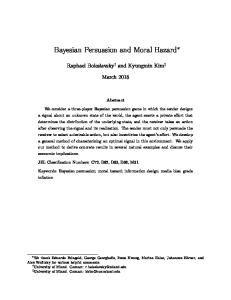
 ( ) = [1 − (0 + ) ]  As a result, banks opt to hoard no liquidity ( = 0) and choose a maximal leverage( =  (0 )). When the crisis is less severe (  ¯ ), then the optimal liquidity choice of banks depends ¯ ()) then continuation on the level of the interest rate  If the interest rate is too high (   does not increase much with every extra unit of hoarded liquidity. As a result, banks again prefer to hoard no liquidity ( = 0) and maximize leverage ( =  (0 )). When the interest rate is low enough, then the elasticity of the continuation scale to hoarded liquidity increases enough to make it worthwhile for banks to reduce their leverage ( =  ()) and set aside enough liquidity ( =  − 0 ) so as to be able to continue at full scale. Equilibrium with optimal ex post bailouts. The following assumption requires that ˆ  () be concave enough. Assumption 5 (enough concavity). The function 2 ˆ 0 () is decreasing in  ∈ [0  1]  We are now in position to characterize the symmetric equilibria of the no-commitment economy. Define  () by the following equation  (1 + 1 − 0 ) 2 () ˆ 0 ( ()) = 0   1 − [ˆ  + (1 −  ˆ ) (1 − )] As we shall see shortly, the interest rate max { ()  0 } corresponds to the equilibrium with the minimal interest rate (in case of crisis) when the fraction of distressed firms is   ¯  Note that  () is decreasing in  and  (0) = 1 Let  be the solution of the equation © ¡ ¢ ª ¡ ¢ ¯   max    0 =  Similarly, define  () by the following equation 2 () ˆ 0 ( ())  (1 − ) (1 − ) = 0   1 − [ˆ  + (1 −  ˆ ) (1 − )] As we shall see shortly, the interest rate max { ()  0 } corresponds to the equilibrium interest rate (in case of crisis) when the fraction of distressed firms is   ¯  Note that  () is increasing in  with  (1) = 1 Finally, let  () ≡ max { ()   ()  0 }  34

Figure 1: Equilibrium interest rate and form of the optimal bailout as a function of the severity of the crisis  Note that  () is first decreasing and then increasing in  Note also that  () is constant and equal to 0 over the (possibly empty) intermediate region where max { ()   ()}  0 . Assumption 6   . If instead  ≥  then there is a unique equilibrium with  =  ()   = 0 and  =  (0 )  Proposition 7 Suppose that Assumptions 1, 3, 5 and 6 hold. The symmetric equilibria of the no-commitment economy are as follows: (i) (bailout with downsizing) if    then there is a unique equilibrium with  =  () = ¯  (),  = 0 and  =  (0 ) ;  (ii) (purely monetary bailout) if      then there is an equilibrium associated with each ¯ ()  with  =  − 0 and  =  ()  value of  between  () = max { ()  0 } and  (iii) (high rents bailout) if    then there is a unique equilibrium with  =  () = max { ()  0 }   = 0 and  =  (0 ) . 35

Proposition 7 and Lemma 1 characterize the equilibrium decision of banks and the form of the optimal bailout as a function of the severity  of the crisis. There is deleveraging in equilibrium (  ) if and only if    in which case  = [0  () + 1 − 0 ]  (1 + 1 − 0 )  Otherwise,  =  and distressed banks continue at full scale. There is a positive transfer   0 to intact banks if and only if   ¯ and  ()  0  in which case  =  [1 − 0  ()]  Turning to the interest rate, recall that the interest rate  () is the equilibrium interest rate where this is a unique equilibrium and the lowest equilibrium interest rate when there are multiple equilibria. As  increases, the interest rate  () is first decreasing  then constant and equal to 0 over the intermediate region where max { ()   ()}  0 and finally increasing on the region where  ()  0  Monetary policy is always used in equilibrium; indeed fiscal bailouts are not even used (in equilibrium) in region (ii); in the remaining regions, monetary policy and fiscal bailouts are used in conjunction. Monetary policy is a market-driven solution, in that it benefits primarily those institutions with actual borrowing needs. Recapitalizations and direct liquidity support better focus on strategic actors, such as commercial banks, but they entail a greater waste of resources by supporting entities that have no need for, or should not engage in refinancing. Interestingly, by increasing the market value of intact institutions, monetary policy discourages the latter from tapping into public funds. When parameters are in the configuration covered by case (ii), there are multiple equilibria. The structure of equilibria resembles the one characterized in Section IV. If banks anticipate a low interest rate, they hoard little liquidity. When a crisis occurs, the authorities find it optimal ex post to set a low interest rate to bail out the banks. Similarly, if banks anticipate a high interest rate, they hoard a lot of liquidity, limiting the ex post incentives for the authorities to lower interest rates if a crisis occurs. Once again banks’ leverage choices are strategic complements. More generally, in this region, the insights gleaned from our analysis of pure monetary bailouts in Sections IV and V carry over to optimal bailouts. It is also instructive to perform comparative statics with respect to the fraction of false positives  When there are few false positives, the authorities face little asymmetric information and choose to give transfers to intact banks to discourage them from claiming to be distressed. Monetary policy is also used to further raise the cost of a deviation, the more so, ¯ ()  max { ()  0 }  when there are a lot of false positives (  ¯), the higher  If  only monetary policy is used: the high fraction of false positives renders direct transfers to intact banks too costly. This corresponds to region (ii) in Proposition 7 and the rationale for

36

© ª ¯ ()  0  This would occur multiple equilibria is identical.23 Instead if that  ()  max  for mild crises (low values of ). The diﬀerence is then that when   ¯ the equilibrium takes the form of a bailout with downsizing. In this case, it is more eﬃcient to downsize distressed banks.24 Remark 3 In practice, participation in a government bailout is likely to come with many strings attached. In our model, this comes in the form of downsizing, but constraints on executive compensation, in particular, also come to mind. This could be formalized as a minor variant of our analysis. Suppose that instead of downsizing (for example, imagine that downsizing is infeasible because the technology is putty-clay) the government imposes constraints on compensation for banks claiming to be distressed. This constraint reduces both the banking entrepreneur’s private benefit 1 −0 , but also the pledgeable income 0 (increased moral hazard, migration of best managers to compensation-unconstrained institutions). The analysis is almost identical.

VII

Conclusion

Finally, we conclude with some reinterpretations and potential extensions of our analysis. Sowing the seeds of the next crisis. In the model, the social cost of bailouts was entirely on the consumer side (subsidies to banks, interest rate distortion). But the logic of our model points at another potential cost, this one on the corporate side. Consider a longer-horizon model, say the overlapping-generations version of this model, in which banking entrepreneurs live, like in this model, for three periods. A monetary bailout at date  + 1 of those banks that borrowed at date  then also aﬀects the financing decisions of the next generation of banks, which borrow at date  + 1. In the appendix, we point out that a low interest rate sows the seeds for the next crisis, and this independently of any reputational concern of the central bank. Interestingly, this operates through two channels: increased ¯ () and  () are independent of  while  () is decreasing in  To underscore this Note that  dependence, we write  ( )  In fact  ( ) is decreasing in  with  ( 0) = 1 For low enough  the equilibrium first takes the form of a high rents bailout with   0  =   = 0 and  =  ( )  When  passes the threshold  where  ( ) =  ()  the£ equilibrium is that of ¤a purely monetary ¯ () with  = 0  =  bailout: there are multiple equilibria, one for each value of  ∈ max { ()  0 }   and  =  − 0  © ª 24 ¯ ()   ()  then the equilibrium always involves  = max { ( )  0 }  ≥ 0 When 0  max   =   = 0 23

37

leverage and increased maturity mismatch. Both channels seem to have operated during the long episode of very low interest rates in the wake of the Internet bubble crash. Consider first the increased leverage channel. By lowering the cost of capital, the central bank creates an investment boom, which will make future rescues more compelling given that, as we have seen, the temptation to lower the interest rate increases with the size of assets to be rescued. Turning to the increased maturity-mismatch channel, note that a reduction in shortterm rates aﬀects liquidity choices. Low short-term rates encourage the banks to hoard less liquidity and therefore to expose themselves to liquidity shortages. A reinterpretation of this result in the context of the short-term debt model presented in Section II is that the date-0 interest rate aﬀects not only the level of borrowing, but also its term structure: banks issue more short-term liabilities and aggravate the maturity mismatch problem.25 Yet another cost of bailouts is the loss of reputation by the central bank. This could be modelled by introducing a tough type and soft type. A big bailout would then reveal the type of the central bank to be soft, raising the likelihood of future bailouts and pushing banks to take on more risk, hoard less liquidity and lever up, resulting in increased economywide maturity mismatch and in turn larger bailouts. Even a central bank of the soft type would internalize these reputational costs and be more reluctant to engage in a bailout in the first place. Similarly the tough type will try to separate itself from the soft type by taking a hard line. Nominal rates. Our modelling of monetary policy deserves some comments. To simplify the exposition and focus on our specific contribution, we have built a real model with no money balances, no sticky prices and no imperfect competition. Yet we argue that our modelling of monetary policy captures a key feature of monetary policy in New-Keynesian models routinely used to discuss and model monetary policy.26 In New-Keynesian models, the nominal interest rate is controlled by the central bank. Prices only adjust gradually according to the New-Keynesian Phillips Curve, and the central bank can therefore control the real interest rate. The real interest rate regulates aggregate demand through a version of the consumer Euler equation — the dynamic IS curve — by determining the slope of the intertemporal consumption profile — the intertemporal rate of substitution. Without additional frictions, the central bank can achieve the allocation of the flexible price economy by 25

A similar point is made in Adrian and Shin (2008). Yet another cost of inflation, absent in cashless New Keynesian models, is the ”inflation tax” and arises when money demand is elastic. 26

38

setting nominal interest rates so that the real interest rate equals to the ”natural” interest rate. Deviating from this rule introduces unnecessary distortions. Our model shares the assumption that monetary policy acts by aﬀecting the real interest rate or equivalently the intertemporal rate of substitution of consumers. However, the specific nature of the distortion imposed by monetary policy is diﬀerent: a wedge between the intertemporal rate of substitution of consumers and the return on the storage technology in our model versus dispersion in relative prices in New-Keynesian model.

39

References [1] Adrian, T. and H.S. Shin (2008), ”Financial Intermediaries, Financial Stability and Monetary Policy”, Jackson Hole. [2] Acharya, V. and T. Yorulmazer (2007), “Too Many to Fail- An Analysis of TimeInconsistency in Bank Closure Policies”, WP 319, Bank of England. [3] Bagehot, W. (1873), Lombard Street: a Description of the Money Market, London: H.S. King. [4] Bernanke, B. and M. Gertler (1995), ”Inside the Black Box: The Credit Channel of Monetary Policy Transmission”, Journal of Economic Perspectives, 9(4), p. 27-48. [5] Cooper, R. (1999), Coordination Games: Complementarities and Macroeconomics, Cambridge, Cambridge University Press. [6] Cooper, R., and A. John [1988], ”Coordinating Coordination Failures in Keynesian Models”, Quarterly Journal of Economics, 103, p. 441-463. [7] Dewatripont, M., and J. Tirole (1994), The Prudential Regulation of Banks, MIT Press. [8] Diamond P. [1982], ”Aggregate Demand Management in Search Equilibrium ”, Journal of Political Economy, 90, p. 881-894. [9] Diamond, D. and R. Rajan (2009), ”Illiquidity and Interest Rate Policy”, mimeo University of Chicago. [10] Freixas, X. (1999), ”Optimal Bailout Policy, Conditionality and Constructive Ambiguity”, LSE FMG discussion paper n◦ 237. [11] Holmstr¨om, B. and J. Tirole, (1997), ”Financial Intermediation, Loanable Funds, and the Real Sector,” Quarterly Journal of Economics, 112(3), p. 663-91. [12] Holmstr¨om, B. and J. Tirole, (1998), ”Private and Public Supply of Liquidity,” Journal of Political Economy, 106(1), p. 1-40. [13] Kashyap, A., R. Rajan and J. Stein (2008), ”Rethinking Capital Regulation”, Jackson Hole. [14] Mailath, G. and L. Mester (1994), ”A Positive Analysis of Bank Closure”, Journal of Financial Intermediation, vol. 3, n◦ 3, p. 272-299. 40

[15] Morris, S., and H.S. Shin (1998), ”Unique Equilibrium in a Model of Self-fulfilling Currency Attacks ”, American Economic Review, 88(3), p. 587-597. [16] Philippon, T. and P. Schnabl (2009), “Eﬃcient Recapitalization”, NBER WP 14929. [17] Ranciere, R., A. Tornell and F. Westermann (2008), ”Systemic Crises and Growth”, Quarterly Journal of Economics, 123(3), p. 359-406. [18] Schneider, M. and A. Tornell (2004) “Balance Sheet Eﬀects, Bailout Guarantees and Financial Crises”, Review of Economic Studies, 71: 883-913.

41

VIII

Appendix

VIII.1

Short-term debt model

In this appendix, we briefly sketch the short-term debt model mentioned in Section II. There are no stores of value at date 0, but the bank receives pledgeable short-term income  at date 1. Without loss of generality, this bank pledges  in the favorable state of nature (probability ) through a combination of safe and contingent short-term debt. The bank also issues safe short-term debt , where 0 ≤  ≤  The cash-flows associated with contingent short-term debt are  −  in the no-crisis state and 0 in the crisis state. Its continuation scale at date 1 in the adverse state of nature is given by  = min

½

¾ ( − ) ,1  1 − 0

Its borrowing capacity at date 0 is given by:  −  −  − (1 − ) − 0  = 0 i.e. =

 1 − 0 −  − (1 − ) 

The banking entrepreneur therefore maximizes over  (1 − 0 ) [ + (1 − )] = (1 − 0 )

"

(−)  + (1 − ) 1−  0

1 − 0 −  − (1 − )

#



which we can rewrite as ∙ ¸ (1 − 0  ( − 0 ) + (1 − )( − )  (1 − 0 ) [ + (1 − )] =  − 0 1 − 0 −  − (1 − ) The banking entrepreneur loads up on short-term debt ( = ) if 1 − 0 −   ( − 0 ) + (1 − ) ≥ (1 − )  (1 − ) 

42

i.e. ≥

1 +

and does not take on short-term debt ( = 0) otherwise.

VIII.2

Proof of Proposition 5

The corresponding planning problem is  ≡ min 

(13)

{()}

s.t. 0 ≤  ( ) ≤ 1 and  R (∗ ) for all ∗ ∈ [0  ) ∗ ∈ The condition for ∗ ∈ [0  ) not to be an equilibrium is that there exists  ∈ (∗  1] such that  ex post (; ∗ ) −  ex post (∗ ; ∗ )  0 or equivalently Z



∗



ex post

³ ´ ∗ ˆ ; 

ˆ 

ˆ  0 

For any given set of values ∆ ( ∗ ) and consider the following subproblem  ({∆ ( ∗ )}) ≡

min

{()}{∆(∗ )}



(14)

s.t. 0 ≤  ( ) ≤ 1 and

Z



∗

³ ´ ˆ ∗  ex post ; ˆ 

ˆ ≥ ∆ ( ∗ ) for all ∗ ∈ [0  1) and  ∈ [∗  1] 

Then the original planning problem (13) and the subproblem (14) are related in the following way: (15)  = min∗  ({∆ ( ∗ )}) {∆( )}

43

s.t. the constraint that for all ∗ ∈ [0  ) there exists  ∈ (∗  1] such that ∆ ( ∗ )  0 Moreover the solution { ( )} of (13) coincides with the solution of (14) when {∆ ( ∗ )} is set as the solution of (15). Turning back to (14) and take {∆ ( ∗ )} to be the solution of (15), the constraint set and the objective function are linear in { ( )} so the first order conditions are necessary and suﬃcient for optimality. Let ∗  ≥ 0 be the multiplier on the constraint Z





ex post

³ ´ ∗ ˆ ; 

ˆ 

∗

ˆ ≥ ∆ ( ∗ )  

Let ¯  ( ) be the multiplier on the constraint  ( ) ≤ 1 and    ( ) be the multiplier on the constraint  ( ) ≥ 0 Finally, let =

X

∗ 

Z



∗

1 ˆ (∗ − 0 )  (∗ ) ³ ´2  ˆ  − 0

The first-order condition for  ( ) is  ( (1))  =   − ¯ +  [ (1 − 0 ) − (1 − 0 )]  The result follows directly from this first-order condition and the complementary slackness conditions    ( ) = ¯ [1 −  ( )] = 0

VIII.3

Proof of Lemma 1

Note that given the interest rate  the planning problem can be decomposed into independent planning problems, one for each value of  and  Consider a given ( )  Suppose first that the incentive compatibility constraint (2 ) is not binding. Then the solution of the planning problem involves  ( ) = 0 and  ( ) =  It can then be verified that (2 ) holds if and only if  ≤ 0 +  This proves (i). Suppose now that   0 +  Then (2 ) is binding and holds as an equality. Using (2 ) to substitute out  ( ) we can therefore rewrite the problem of choosing  ( ) and  ( ) as follows: ¸  −  (1 − ) (1 − )  ( ) max 1 + 1 − 0 ∙

44

subject to min

½

¾   1  ≤  ( ) ≤   − 0

and  ( ) ≥

0 + 

+ 1 − 0  1 + 1 − 0

where the last constraint is a reformulation of ( 1 ) There are two cases to consider. If   ¯  then the solution is to set  ( ) =  This implies  ( ) =  [1 − (0 + ) ]  This proves (ii). ¾ ½ 0 + +1 −0    Note that for all If   ¯  then the solution is to set  ( ) = max −  1+ − 0

 ∈ [0  − 0 ]

1

0

0 + 

+ 1 − 0  ≥  1 + 1 − 0  − 0

Hence, the solution involves

 ( ) =

0 + 

+ 1 − 0  1 + 1 − 0

This implies  ( ) = 0 This proves (iii).

VIII.4

Proof of Lemma 2

It is easy to see that the bank would never choose to set    − 0 . Suppose first that  (1 + 1 − 0 )   (1 − ) (1 − )  Then ¸ ∙ 0 +    ( ) =  and  ( ) =  1 − 

The utility of the banking entrepreneur is given by ¤ £ 1 + (1 − ) 1 − 0+ (1 − 0 )  1 + (1 − )  − 0 which is decreasing in  This proves (iii). Suppose now that  (1 + 1 − 0 )   (1 − ) (1 − )  Then  ( ) =

0 + 

+ 1 − 0  and  ( ) = 0 1 + 1 − 0 45

The utility of the banking entrepreneur is

(1 − 0 ) 

 + (1 − )

0 + +1 −0 

1+1 −0

1 + (1 − )  − 0

¯ () and decreasing in  if    ¯ ()  This proves (i) and which is increasing in  if    (ii).

VIII.5

Proof of Proposition 7

We consider the planning problem for degenerate distribution  ( ) where the distribution has full mass at ( )  For the value of ( ) under consideration, let  be the multiplier on the incentive constraint (2 ),  the multiplier on the participation constraint ( 2 ), ¯ the multiplier on the scale constraint (11) and  the multiplier on the participation constraint ( 1 ). We denote by  and  the values of  ( ) and  ( ) for the value of ( ) under consideration. The first-order conditions for   and  are  2 2 ˆ 0 () =−  (0 + )  (0 + ) ( − 0 )2  ¯ −  =+ 1 + 1 − 0 1 + 1 − 0

and

 (1 − ) (1 − ) =  +  The solution for the interest rate is: ( ) 2 ˆ0 0 ˆ   () ( + )  (0 + )    (1 − ) (1 − )  0 = min  (0 + )  1 + 1 − 0  If  = min 1 + 1 − 0 then

(

 ( + ) ˆ 0 (0 + )   (1 − ) (1 − )  0 1 + 1 − 0   2 ˆ 0 () = (0 + )  1 + 1 − 0

46

)

and =

0 + 

+ 1 − 0 ,  = 0 1 + 1 − 0

If (0 + ) ˆ 0 (0 + ) = min  then

(

( + ) ˆ 0 (0 + )    (1 − ) (1 − )  0 1 + 1 − 0 

2 ˆ 0 () ( + ) ˆ 0 (0 + ) = 0 (0 + )  

and = Finally if  (1 − ) (1 − ) = min then

and

(

i.e.

)

 = 0 + 

0 + 

+ 1 − 0  and  = 0 1 + 1 − 0

( + ) ˆ 0 (0 + )    (1 − ) (1 − )  0 1 + 1 − 0 

)

2 ˆ 0 () =  (1 − ) (1 − ) (0 + )  ¸ ∙ 0 +    = ,  =  1 − 

The proposition follows directly from combining these results with those of Lemma 2.

VIII.6

Date-0 interest rate

Consumer preferences are now (0 ) + (1 ) + 2 . Let 0 denote the economy-wide interest 0 0 0 rate between dates 0 and 1 (0 =  (0 ) (1 )) and, as earlier,  =  (1 ). We first present the model with liquidity and stores of value and then the model with short-term debt. The borrowing capacity at date 0 is given by  −  +  =

 (0 + )  0 

47

The direct eﬀect on scale of a lower date-0 interest rate can be seen by noting that for a given  scale  increases with 0  We now turn to the eﬀect of lower interest rate on the severity of the maturity mismatch problem, indexed by the liquidity choice of banking entrepreneurs. The banking entrepreneur therefore maximizes over  ≤  − 0 :

⎤   + (1 − ) − 0 ´ ⎦  ³ (1 − 0 ) [ + (1 − )] = (1 − 0 ) ⎣ 0  1 − 0  + 1 − 0   ⎡

The banking entrepreneur chooses to hoard enough liquidity to withstand a crisis ( =  − 0 ) if 1 − 0 0  ( − 0 ) ≤ 1− 1 − 0  and no liquidity ( = 0) otherwise. It is easy to see that the right-hand side of this equation is increasing in 0  so that a lower date-0 interest rate 0 discourages liquidity hoarding and increases the maturity mismatch problem. We now briefly turn to the version of the model with short-term debt, which illustrates the same eﬀects. There are no stores of value at date 0, but the bank receives pledgeable short-term income  at date 1. Without loss of generality, this bank issues short-term debt equal to  in the favorable state of nature (probability ) in which it has no reinvestment need, and , where 0 ≤  ≤  in the state of nature in which it has to re-invest 1 for 1 (probability 1 − ).The borrowing capacity at date 0 is given by: −−

   − (1 − ) −  0 = 0 0 0 0 

The banking entrepreneur therefore maximizes over  ⎡

(1 − 0 ) [ + (1 − )] = (1 − 0 ) ⎣

 + (1 − ) (−)  1− 0 

1−

 0

− (1 − ) 0 −

0 0 

⎤

⎦

The banking entrepreneur loads up on short-term debt ( = ) if  +  ≥ 0 and does not take on short-term debt ( = 0) otherwise. Thus a low short-term interest

48

rate 0 increases the scale of investment  and encourages the bank to engage in maturity mismatch.

49