Constraint-based Learning for Text Categorization Savatore Frandina and Claudio Sacc`a and Michelangelo Diligenti and Marco Gori 1 Abstract. Text categorization automatically assigns a document to its underlying topics. Documents are typically represented as bag-ofwords, and machine learning based approaches have been shown to provide effective and scalable solutions by learning from examples. However, a limiting factor in the application of these approaches relies on the large number of examples required to train a classifier working on large taxonomies of classes. This paper presents a method to integrate prior knowledge that is typically available on the learning task into a text classifier based on kernel machines. The presented solution deals with any prior knowledge represented as firstorder logic (FOL) and, thanks to the generality of this formulation, can be used to express relations among the input patterns, known semantic relationships among the output categories and input-output rules. The kernel machine mathematical apparatus is re-used to cast the learning problem into a primal optimization of a function composed of the loss on the supervised examples, the regularization term, and a penalty term deriving from converting the knowledge into a set of continuous constraints. The experimental results, performed over the popular CORA dataset, show that the proposed approach overperforms both SVMs and state-of-the-art semi-supervised techniques in multi-label text classification problem.

1

Introduction

Text categorization decides the topics of a document based on its representation. Documents are typically represented as bag-of-words, and classical machine learning tools can be used to perform the classification after having trained a model from examples. SVMs, a special class of kernel machines, have been proved to be one of the most versatile machine learning approaches to text categorization, providing near state-of-the-art accuracy on many datasets while requiring little tuning. This paper presents a novel method to perform text categorization using any prior knowledge available. The approach is based on a framework that integrates kernel machines and logic to solve multi-task learning problems. The kernel machine mathematical apparatus allows casting the learning problem into a primal optimization of a function composed of the loss on the supervised examples, the regularization term, and a penalty term deriving from forcing the constraints converting the logoc. This naturally allows to get advantage of unsupervised patterns in the learning task, as the degree of satisfaction of the constraints can be measured on unsupervised data. This paper assumes that prior knowledge is available both in terms of know relations among the input patterns (as it happens for Web documents connected via hyperlinks or scientific papers connected via citations), known semantic relationships among the output categories (for example to model an ontology) and in terms of inputoutput rules. We assume that this knowledge can be represented in 1

Dipartimento di Ingegneria dell’Informazione, Universit`a di Siena, Italy, email: {claudio.sacca,frandina,michi,marco}@dii.unisi.it

first-order logic (FOL). The connections between logic and machine learning have been the subject of many investigations, like [1] which studies the relationships between symbolic and sub-symbolic models in AI. A broader coverage of the field with emphasis on the connections with inductive logic programming is in [2]. A related approach to combining first-order logic and probabilistic graphical models in a single representation are Markov Logic Networks [3]. In [4], the well-known inductive logic programming system FOIL is combined with kernel methods by leveraging FOIL search for a set of relevant clauses. This model, called kFOIL, can be used to solve either classification or regression tasks. However, one main limitation of the reviewed approaches is the lack of tight integration between the machine learning which deals with the perceptual representation of the patterns and the prior knowledge on the patterns and classes. The only direct attempt [5] is limited to rules on the perceptual space (input-output). The idea of centering the theory around the general and unified notion of constraints turns out to be a very straightforward way of bridging logic and kernels, since it is possible to express most classic logic formalisms by constraints and supervised examples as used in most learning machines are just a special instance of (soft) constraints. The experimental results, performed over the popular CORA dataset, confirm that the proposed approach performs better than supervised (SVMs) and semi-supervised (Laplacian SVM, Transductive SVM) approaches in a multi-label classification problem. The paper is organized as follows: the next section introduces learning from constraints with kernel machines. The translation of any FOL knowledge into real-valued constraints is described in section 3, and some experimental results are reported in section 4. Finally some conclusions and are drawn.

2

Learning with constraints

We consider a multitask learning problem in which the input is a tuple X = {xj |xj ∈ Dj , j = 1, . . . , n}, being Dj the domain of the values for the j-th attribute. The learning task considers a set of functions {τk (xj(1,k) , . . . , xj(nk ,k) )|k = 1, . . . , T, xj(l,k) ∈ X , τk ∈ Tk } taking a subset of the data as input. Some of the functions may be known a priori whereas others must be inferred from examples. In general, we assume that the attributes in each domain are described by a real valued vector of features that are relevant to solve the tasks at hand. Hence, it holds that Dj = IRdj and τk : IRdj(1,k) ×. . .×IRdj(nk ,k) → IR. For the sake of compactness, in the following weP will indicate by xk = [x0j(1,k) . . . x0j(nk ,k) ]0 ∈ IRdk , where dk = l=1,...,nk dj(l,k) , the input vector for the k-th task. We consider the case when the tasks functions τk have to meet a set of constraints that can be expressed by the functionals φh : T1 × . . . × TT → [0, +∞) such that φh (τ1 , . . . , τT ) = 0 h = 1, . . . , H must hold for any valid choice of τk ∈ Tk , k = 1, . . . , T .

In order to define the learning task, we suppose that each task function τk can be approximated by a fk in an appropriate Reproducing Kernel Hilbert Space Hk . Therefore, the learning procedure can be cast as an optimization problem that aim at computing the optimal functions f1 ∈ H1 , . . . , fT ∈ HT , where fk : IRdj(1,k) × . . . × IRdj(nk ,k) → IR, k = 1, . . . , T . In the following, we will indicate by f = [f1 , . . . , fT ]0 the vector collecting these functions. We consider the classical learning formulation as a risk minimization problem. Assuming that the correlation among the input features xk and the desired task function output yk is modeled by a joint probability distribution p(xk ,yk ) (xk , yk ), the risk associated to a hypothesis f is measured as, Z T X R[f ] = λτk · Lek (fk (xk ), yk ) p(xk ,yk ) (xk , yk ) dxk dyk

In general, the functionals φh (f ) implementing the constraints involve all the values computed by the functions in f on their whole domains making training difficult. Hence, as in the case of the risk, we assume that these functionals can be conveniently approximated by considering an appropriate sampling in the function domains. In particular, the exact constraint functional will be replaced by an approximation exploiting only the values of the unknown functions f computed for the points in U: φh (f ) ≈ φˆh (U, f ). Thus, the given learning problem is cast in a semi-supervised framework where it is assumed that a set of (partially) labeled examples is exploited together with a lset of unlabeled examples. Given the available supervised examples in Lk and an unsupervised sample Uk , k = 1, . . . , T , the objective function considering the empirical risk and the empirical penalty is,

k=1

Eemp [f ]

where λτk > 0 is the weight of the risk for the k-th task and Lek (fk (xk ), yk ) is a loss function that measures the fitting quality of fk (xk ) with respect to the target yk . Common choices for the loss function are the quadratic function especially for regression tasks, and the hinge function for binary classification tasks. PT r The regularization term can be written as N [f ] = k=1 λk · 2 r ||fk ||Hk , where λk > 0 can be used to weight of the regularization contribution for the k-th task. Clearly, if the tasks are uncorrelated, the optimization of the objective function R[f ] + N [f ] with respect to the T functions fk ∈ Hk is equivalent to T stand-alone optimization problems for each function. However, if we consider a problem for which some correlations among the tasks are known a priori and coded as rules, we can enforce also these constraints in the learning procedure. Following the classical penalty approach for constrained optimization, we can embed the constraints by adding a term that penalizes their violation. Since the functionals φh (f ) are strictly positive when the related constraint is violated and zero otherwise, the overall degree of constraint violation of the current hypothesis f can be measured as V [f ] =

H X

λvh · φh (f ) ,

h=1

where the parameters λvh > 0 allow us to weight the contribution of each constraint. It should be noticed that, differently from the previous terms considered in the optimization objective, the penalty term involves all the functions and, thus, explicitly introduces a correlation among the tasks in the learning statement. Finally, we can add together all the contributions yielding the objective E[f ] = R[f ] + N[f ] + V[f ]. Since the distributions p(xk ,yk ) (xk , yk ), k = 1, . . . , T needed to determine R[f ] are usually not known, we apply the common assumption to approximate them through their empirical realizations. This requires to have a set of examples drawn from these unknown distributions. Basically, the learningset will
contain a set of labeled examples for each task k: Lk = xik , yki |i = 1, . . . , `k . The i unsupervised examples are
collected in Uk = {xk |i = 1, . . . , uk }, L while Sk = {xk | xk , yk ∈ Lk } collects the sample points that are in the supervised set for the k-th task. The set of the S supervised and unsupervised points for the k-th task is Sk = SkL Uk . Given an input object we can assume that also a partial labeling can be provided, i.e. it is not required to specify the targets for all the considered tasks for each sample corresponding to the i-th instance X i of the input tuple. In the following we will refer to the unsupervised set U = {X i |∃k : xik ∈ Uk }.

=

T X λτk |Lk |

k=1

+

T X

λrk

·

  Lek fk (xjk ), ykj +

X xjk ,ykj




∈Lk

||fk ||2Hk

+

k=1

3

(1)

H X

λvh

· φˆh (U, f ) .

h=1

Translation of first-order logic clauses into real-valued constraints

We focus attention on knowledge-based descriptions given by firstorder logic (FOL–KB). In the following, we indicate by V = {v1 , . . . , vN } the set of the variables used in the KB, with vs ∈ Ds . Given the set of predicates used in the KB: P = {pk |pk : Ds(1,k) × . . . × Ds(nk ,k) → {true, f alse}, k = 1, . . . , T }, the clauses will be built from the set of atoms A = pk(i) (vs(1,k(i)) , . . . , vs(nk(i) ,k(i)) )|i = 1, . . . , m, pk(i) ∈ P, vs(j,k(i)) ∈ V , where the i-th atom is an instance of the k(i)th predicate for which the j-th argument is assigned to the variable vs(j,k(i)) ∈ Ds(j,k(i)) . In the following, for the sake of compactness, we will indicate by v ai = [vs(1,k(i)) , . . . , vs(nk(i) ,k(i)) ] the argument list of the atom ai ∈ A. With no loss of generality, we restrict our attention to FOL clauses in the PNF form, where all the quantifiers (∀, ∃) and their associated quantified variables are placed at the beginning of the clause. The quantifier-free part of the expression is equivalent to an assertion in propositional logic for any given assignment of the quantified variables. Since any propositional expression can be written in Conjuctive Normal Form (CNF), we can assume that all FOL expressions are in PNF-CNF form, Quantifier-free CNF expression E0 (vE0 , P)

z  Quantified Portion }| { ^ z  [∀∃]vs(1) . . . [∀∃]vs(Q) c=1,...,C

}| _

{

[¬] ai(c,d) (vai(c,d) ) ,

d=1,...,Dc

where ai(c,d) ∈ A is an atom and the variables vs(q) ∈ V, q = 1, . . . , Q constitute the set of the quantified variables. The quantifierfree expression E0 (v E0 , P) depends on the list of arguments v E0 = [vs(1,E0 ) , . . . , vs(nE0 ,E0 ) ] corresponding to the variables used in all the atoms ai(c,d) , i.e. vs(j,E0 ) ∈ {vq ∈ V|∃c, d vq ∈ args(ai(c,d) )} where args(ai(c,d) ) is the set of the variables vai(c,d) used as arguments in the atom ai(c,d) . We assume that the task functions fk are exploited to implement the predicates in P and each variable in V maps to the attributes defining the tuple X on which the functions fk are defined.

The FOL–KB will contain a set of clauses corresponding to expressions with no free variables (i.e. all the variables appearing in the expression are quantified) that are assumed to be true in the considered domain. These clauses can be converted into a set of constraints as in that can be enforced during the kernel based learning process. The conversion process of a clause into a constraint functional consists of the following three steps:

A=>B

1

0.5

0 1

I. P REDICATE SUBSTITUTION: substitution of the predicates with their continuous implementation realized by the functions f composed with a squash function, mapping the output values into the interval [0, 1] such that the value 0 is associated with false and 1 with true.. In particular, the atom ai (v ai ) is mapped to σ(fk(i) (v ai )), where σ : IR → [0, 1] is a monotonically increasing squashing function. A natural choice for the squash function is the piecewise linear mapping σ(y) = min(1, max(y, 0)), this is indeed the function that was employed in the experimental results. II. C ONVERSION OF THE P ROPOSITIONAL E XPRESSION: conversion of the quantifier-free expression where all atoms are grounded as detailed in subsection 3.1. In our context the propositional logic clause to be generalized into a continuous function is grounded with the output values of the functions applied on a pattern (if unary), or on a vector of patterns if n-ary. III. Q UANTIFIER CONVERSION: conversion of the universal and existential quantifiers as shown in section 3.2.

3.1

Logic expressions and their continuous representation

As studied in the context of fuzzy logic and symbolic AI, different methods can be used for the conversion of a propositional expression into a continuous function with [0, 1] input variables. T-norms. In the context of fuzzy logic, t-norms [6] are commonly used as a generalization of logic clauses to continuous variables. A t-norm is a function t : [0, 1] × [0, 1] → IR, that is commutative, associative, monotonic and featuring a neutral element 1 (i.e. t(x, 1) = x). A t-norm fuzzy logic is defined by its t-norm t(x, y) that models the logic AND and a function modeling the negation of a formula. For example, the negation of x corresponds to 1 − x in the Lukasiewicz norm. Many different t-norm logics have been proposed in the literature like the product t-norm t(x, y) = x · y and the minimum t-norm defined as t(x, y) = min(x, y). Once defined the t-norm functions corresponding to the logical AND and NOT, these functions can be composed to convert any arbitrary logic proposition.

1 f

b

f

a

0

0

a. A=>B

1

0 1

1

fa

fb 0

0

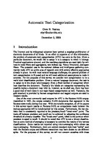
b. Figure 1: Function resulting from the conversion of a ⇒ b using PGAUSS (a.) and NGAUSS (b.).

where x = [x1 , . . . , xn ] is a vector containing the variables in the clause and T is the set of all possible configurations of the input variables corresponding to a true truth value. We indicate as P GAU SS this conversion procedure. The value of t(x, y) will decrease depending on the distance from the closest configuration verifying the clause. Each configuration verifying the constraint is always a global maximum of t when using a small enough σ value. See [7] for a complete discussion on how to select σ. An alternative approach, that we indicate as NGAUSS, is to represent the false values of the truth table of the clause. In this case, one negative Gaussian is centered on each configuration of variables yielding a false value of the considered clause. A bias value equal to 1 is introduced to obtain a default true value when distant from a false configuration: t(x) = 1 −

X

 ||[x , . . . , x ]0 − [c , . . . , c ]0 ||2  1 n 1 n , exp − 2σ 2

[c1 ,...,cn ]∈F

Mixture of Gaussians. A different approach based on mixtures of Gaussians has been proposed in [7] in the context of symbolic learning using neural networks. Unlike t-norms, this approach generalizes the logic clause without making any independence assumption among the variables. In particular, let us consider a propositional logic clause involving n logic variables. The logic clause is equivalent to its truth table containing 2n rows, each one corresponding to a configuration of the variables. The continuous function approximating the clause is based on a set of Gaussian functions, each one centered on a configuration corresponding to the true value in the truth table. The mixture function sums all the Gaussians:   X ||[x1 , . . . , xn ]0 − [c1 , . . . , cn ]0 ||2 t(x) = exp − 2σ 2 [c1 ,...,cn ]∈T

where F is the set of input configurations corresponding to a false value in the truth table. Figure 1 shows the functions obtained by converting the clause a ⇒ b using PGAUSS and NGAUSS. Any formula can be converted using both forms but, depending on the formula, one mixture can be more compact. Hypercube. This class of conversion methods considers the ndimensional space formed by associating each logic propositional variable in a clause to a dimension of the space. This builds a hypercube associating each configuration of the variables in the truth table to a vertex. Let tt(c) be a function mapping a configuration c = [c1 , . . . , cn ] to its truth value: tt(c) = 1 if c ∈ T and tt(c) = 0 if c ∈ F. Let’s now consider a continuous generalization of the logic

variables in the [0, 1] range. The generalized truth value of a point x can be computed as weighted average of the values in the vertices: P n t(x) = 2k=1 wk (x) · tt(ck ) where ck is a tuple corresponding to k-th configuration in the truth table. Depending on the selection of the weights wk (x) different conversion schema are obtained. For example, the Hypercube-Closest-Vertex norm selects the truth value of the closest vertex as:  D(x,ck ) D(x,ck ) ≤ D(x,cj ) j=1,. . .,2N, j 6= k wk (x)= 0 otherwise where D(x,ck ) is the Euclidean distance between x and vertex ck . The Hypercube-Distance norm weights vertices inversionally proportional to the generalized Hamming distance from the input x: wk (x) =

n Y

|cki − ci |

where cki is the i-th element of ck . The main advantage of this latter norm is that any point in a hyperplane merging two or more vertexes with the same truth value tt will also be assigned to tt. For example, when converting the rule A ⇒ B ∧ C, any of the 4 vertexes corresponding to A = 0 are associated to a true value in the truth table (e.g. tt(0, c1 , c2 ) = 1). Therefore, t(0, x1 , x2 ) = 1 for any x1 = [0, 1], x2 = [0, 1] meaning that any point on the hypercube face will satisfy the constraint. This property allows to build constraints that are easier to satisfy as they do not introduce any unnecessary requirement. Any of the above norms allow the mapping of any arbitrary quantifier-free expression E(v E , P) to a functional constraint can be written ϕE (v E , f ) = 0, depending on all the variables collected in the argument list v E = [vs(1,E) , . . . , vs(nE ,E) ] and on the predicates implemented by the functions f .

The quantified portion of the expression is processed recursively by moving backward from the inner quantifier in the PNF expansion. Let us consider the universal quantifier first. The universal quantifier expresses the fact that the expression must hold for any realization of the quantified variable vq . When considering the real–valued mapping of the original boolean expression, the universal quantifier can be naturally converted measuring the degree of non-satisfaction of the expression over the domain Dj(q) where the feature vector xj(q) , corresponding to the variable vq , ranges. This measure can be implemented by computing the overall distance of ϕE (v E , f ), that is the degree of violation associated to the quantified expression, from the constant function equal to 0 (this is the only value for which the constraint is always verified), over the domain Dj(q) . Measuring the distance using the infinity norm yields sup

|ϕE (v E , f )| , (2)

vq ∈Dj(q)

where the resulting expression depends on all the variables in v E except vq . Hence, the result of the conversion applied to the expression Eq (v Eq , P) = ∀vq E(v E , P) is a functional ϕEq (v Eq , f ), assuming values in [0, 1] and depending on the set of variables v Eq = [vs(1,Eq ) , . . . , vs(nEq ,Eq ) ], such that nEq = nE − 1 and vs(j,Eq ) ∈ {vr ∈ V|∃i vr = vs(i,E) , vr 6= vq }. The variables in v Eq need to be quantified or assigned a specific value in order to obtain a constraint functional depending only on the functions f .

→

inf vq ∈Dj(q) ϕE (v E , f )

Unfortunately, it is generally complex to compute the exact expression for the functionals since the conversion of the quantifiers requires to extend the computation on the whole domain of the quantified variables. We assume that the computation can be approximated by exploiting the available empirical realizations of the feature vectors. Hence, the quantifiers exploiting the infinity norm are approximated using the empirical distribution Sxj for the feature xj as: ∀vq E(v E , P)

→

max

vq ∈Sx

|ϕE (v E , f )|

j(q)

∃vq E(v E , P)

→

min

vq ∈Sx

|ϕE (v E , f )| .

j(q)

In description logics, it is common to define an ∃n operator, which generalizes the existential operator to from one to n elements. While FOL can also indirectly express ∃n , it may be convenient and more compact to provide a direct translation of the ∃n operator as: ∃n vq E(v E , P)

Quantifier conversion

∀vq E(vE , P) → kϕE (v E , f )k∞ =

Proof: See [8]. Theorem 1 shows that there is a duality between an universally quantified expression and its continuous generalization. If we consider the conversion of the PNF representing a FOL constraint without free variables, the variables are recursively quantified until the set of the free variables is empty. In the case of the universal quantifier we apply again the mapping described previously. The existential quantifier can be realized by starting from eq. (2), and enforcing the De Morgan law (∃vq E(v E , P) ⇐⇒ ¬∀vq ¬E(v E , P)) to hold also in the continuous mapped domain: ∃vq E(v E , P)

i=1

3.2

Theorem 1. Let E(v, P) be an FOL expression with no quantifiers depending on the variable v. Let tE (v, f ) be the continuous representation of E, where fk corresponds to pk , k = 1, . . . , T . If fk ∈ C0 , k = 1, . . . , T , then k1 − tE (v, f )kp = 0 iff ∀v E(v, P) is true.

→

min(n)vq ∈Sxj(q) |ϕE (v E , f )| ,

where min(n) is the n-th minimum value over the set. It is possible ti use a different norm to convert the universal quantifier, for example using norm-1: X ∀vq E(v E , P) → |ϕE (v E , f )| . vq ∈Sx

j(q)

Please note that ϕE ([], f ) will always reduce to a form that depends on the realizations of the functions over the data point samples. The solution to the optimization task defined by equation 1 with constraints evaluated over a finite set of data points can be computed by considering the following extension of the Representer Theorem [9], see [8] for details and a proof. Theorem 2. Given a multitask learning problem for which the task functions f1 , . . . , fT , fk : IRdk → IR, k = 1, . . . , T , are assumed to belong to the Reproducing Kernel Hilbert Spaces H1 , . . . , HT , respectively, and the problem is formulated as [f1∗ , . . . , fT∗ ] = argminf1 ∈H1 ,...,fT ∈HT Eemp [f1 , . . . , fT ] where Eemp [f1 , . . . , fT ] is defined as in equation (1), then each function fk∗ in the solution can be expressed as X ∗ fk∗ (xk ) = wk,i Kk (xik , xk ) i xk ∈Sk where Kk (x0k , xk ) is the reproducing kernel associated to the space Hk , and Sk is the set of the available samples for the k-th function.

Therefore, the optimal solution can be expressed as a kernel expansion over the data points. In fact, since the constraint is represented by ϕE ([], f ) = 0 in the definition of the learning objective ˆ function, it is possible to substitute φ(U, f ) = ϕE ([], f ).

3.3

Special cases

Transductive SVMs [10] correspond to a special case of the proposed framework, where a logic clause imposes that any predicate should be either true or false. While this rule is always verified in standard logic, it is not verified in fuzzy logics. Therefore, ∀x P (x) ∨ ¬P (x) forces function fP estimating predicate P to assume values that are away from the separating surface even on unsupervised data. As typically done in Transductive SVMs, it is possible to avoid unbalanced solutions by imposing that ∃n x P (x) ∧ ∃m x ¬P (x) : n + m = N where N is the total number of patterns and n and m are estimated P P from the supervised examples: n = N · nP pos /(npos + nneg ) where P P npos and nneg are the number of positive and negative supervised examples for predicate P , respectively. Manifold regularization [11] assumes that the classification functions should be regular over the manifold built over the input data distribution. Laplacian SVMs are a effective semi-supervised approach to train SVMs under the manifold regularization assumption. Let us introduce a predicate R(x, y) which holds true if and only if x, y are connected on the manifold. R is typically a known predicate which is built using geometrical properties. The manifold assumption in a logic setting, where two connected points should either both true or false can be expressed as: ∀x R(x, y) ⇒ (P (x) ∧ P (y)) ∨ (¬P (x) ∧ ¬P (y)) .

3.4

Stage-based learning

The optimization of the overall error function is performed in the primal space using gradient descent [12]. Unlike when only considering supervised examples, the objective function is non-convex due to the constraint term. In order to face the problems connected with the presence of sub-optimal solutions, the optimization problem was split in two stages. In a first phase, as commonly done by kernel machines it is performed regularized fitting of the supervised examples. Only in a second phase, the constraints are enforced since requiring a higher abstraction level. This solution has intriguing connections with results of developmental psychology, since it is well-known that many animals experiment stage-based learning [13]. From a pure optimization point of view, the first stage with the correspondent guarantee of convergence to an optimal solution makes possible to approach the global basin of attraction, while the second stage refines learning beginning from a good initialization. The different constraints can also be gradually introduced. As common practice in constraint satisfaction tasks, more restrictive constraints should be enforced earlier. As metric of how restrictive a logic constraint is, it is possible to use the portion of true configurations of the corresponding clause.

4

Experimental results

The experimental results have been carried out on a subset of the CORA dataset 2 . The CORA dataset is composed by a set of entities and their relations to allow experimenting with machine learning approaches which can cope with relations. Entities are authors and scientific papers, even if only papers are considered in our experimental setting. CORA assigns to each paper a set of categories (multi-label classification task), selected from a taxonomy of classes. The goal of our experiments is to predict the categories assigned to each paper. For our experiments, we have created a dataset of scientific publications by selecting the 3 first-level (in the taxonomy) categories which have the highest number of papers. Then all the papers in the child classes of the selected higher level classes have been selected as well. All the papers not belonging to at least one of these categories have been discarded, from the remaining papers a random sample of 1000 papers has been performed. Each paper is then associated with a vectorial representation containing its title represented as bag-ofwords. We assume that each category is associated to a predicate, taking a paper as input, which holds true if and only if the paper belongs to the category. We indicate as Ci (·) the predicate for the i-th class of the dataset. Five folds have been generated by selecting n% of the papers for which supervisions are kept (n=10,20,30,40 over different experiments) as training set. 15% of the papers of the initial dataset have been been inserted into the validation set, while the remaining papers have been removed of the supervisions and used for testing. The knowledge base collects different collateral information which is available on the dataset. For example, CORA makes available a list of citations for each papers, our algorithm can exploit these relations assuming that a citation represents a common intent between the papers that are therefore suggested to belong to the same set of categories. This can be expressed via a set of 10 clauses (one per category) such that foreach i = 1, . . . , 10: ∀x ∈ P ∀y ∈ P Cite(x, y) ⇒ (Ci (x)∧Ci (y))∨(¬Ci (x)∧¬Ci (y)) where P is the domain of all papers in the dataset and Cite(x, y) is a binary predicate which holds true iff paper x cites paper y. This set of clauses will smooth the value of the estimated predicates over the citation graph. This effect is very similar to what would be done by manifold regularization or other similar techniques [14].

SVM

SBR

TSVM

LSVM

Recall Precision F1 Recall Precision F1 Recall Precision F1 Recall Precision F1

10% 0.473 0.714 0.569 0.672 0.673 0.672 0.617 0.602 0.608 0.615 0.669 0.641

20% 0.521 0.756 0.617 0.692 0.741 0.715 0.672 0.677 0.674 0.660 0.744 0.699

30% 0.576 0.793 0.667 0.741 0.773 0.756 0.696 0.695 0.695 0.702 0.770 0.734

40% 0.624 0.796 0.700 0.770 0.804 0.787 0.725 0.711 0.718 0.738 0.814 0.774

Table 1: Precision, recall and F1 metrics averaged over 5 runs using SVM, Transductive SVM (TSVM), Laplacian SVM (LSVM) and Semantic Based Regularization (SBR) using only citation and taxonomic constraints varying the number of supervised patterns. Metrics in bold represent statistically significant gains (95%) over all the other classifiers.

2

Download at http://people.cs.umass.edu/∼mccallum/data.html

Other clauses can be inserted to model the relationships among the classes. For example, the CORA taxonomy can be used to build clauses stating that if the predicate associated to a leaf node is true, then all the predicates associated to the nodes up to the root should be true as well: ∀ x ∈ P Ci (x) ⇒ pa [Ci ] (x) where pa [Ci ] is the father category of Ci in the taxonomy. Furthermore, the following rule defines a close world assumption ∀ x ∈ P c1 (x) ∨ c2 (x) ∨ c3 (x), where c1 , c2 , c3 are the three classes in the first-level of the taxonomy. Overall, a total number of 8 clauses was used to model the taxonomy. Other external semantic knowledge can be inserted as well using common knowledge about the environment. For example, let HasW ord be a given predicate holding true iff document x has word ”neural”, it is possible to associate the presence of the term to either the category Artificial Intelligence or Biology as: ∀ x ∈ P HasW ord(x, N eural) ⇒ Cai (x) ∨ Cbio (x) where Cai , Cbio indicate the predicate for Artificial Intelligence, and biology, respectively. 45 clauses of this kind have been added to the knowledge base. The logic translation of the transductive rule as described in section 3.3 can also be added for each category (10 total). Therefore, the overall knowledge base is composed of 93 FOL clauses3 . In our experimental setting, the Hypercube-distance norm has been use to convert all clauses, except the transductive rules for which the Hypercube-Nearest-Vertex norm has been employed. The norm-1 has been used to convert all clauses, except for citations rules for which the infinity norm was used. Stage-base learning was used to train all the SBR classifiers.

SVM (using only the supervised labels), a Transductive SVM (implemented in the svmlight software package) and Laplacian SVM using the citations to build the manifold of data. When training with the knowledge base the stage-based procedure described in section 3.4 has been used. The validation set has been used to select the best values for λr and λc (same value for each function e.g. λr = λri i = 1, . . . , 10 and λc = λci i = 1, . . . , 10). The precision, recall and F1 results have been compute as an average over five different samples of the dataset. Table 1 summarizes the results for a different number of supervised data when using only citations and taxonomic logic clauses. SBR provides a statistically significant F1 gain for two datasets over four and the highest average F1 score for the other datasets. Figure 2 shows a detailed breakdown of the effect of the single rules on the 10%-supervised dataset as an average over five runs. Citation, transductive, taxonomy and input-output constraints all contribute to improve over standard SVMs. However, F1 is maximized when all constraints are added at the same time. All the SBR classifiers combining multiple clauses provide gains over SVM, TSVM and LSVM that are statistically significant (95%).

5

Conclusions and future work

This paper presents a text categorization approach, which is able to provide a tight integration of prior knowledge and the classical kernel machine apparatus. The approach is very general, as any knowledge expressed in FOL can be considered, including relational knowledge among patterns and classes, semantic knowledge like ontologies and input-output rules. The experimental results have been carried out on the CORA dataset and they show the effectiveness of the proposed approach on a multi-label classification problem.

REFERENCES

Figure 2: F1 (average over five runs) using SVM, TSVm , LSVM and SBR with different set of rules: taxonomic (T), citation (C), transductive (TR), input-output rules (IO) and different combinations of these over the dataset with 10% supervised.

For each subsample size of the training set, one classifier has been trained. As a comparison, we also trained for each set a standard 3

The vectorial representation of the patterns (both in SVMlight and our format) and the list of rules in a format suitable for our software simulator can be downloaded (together with the full software bundle) from https://sites.google.com/site/semanticbasedregularization/home

[1] P. Hitzler, S. Holldobler, and A. K. Sedab, “Logic programs and connectionist networks,” Journal of Applied Logic, vol. 2, no. 3, pp. 245– 272, 2004. [2] L. D. Raedt, P. Frasconi, K. Kersting, and S. M. (Eds), Probabilistic Inductive Logic Programming, vol. 4911. Springer, Lecture Notes in Artificial Intelligence, 2008. [3] M. Richardson and P. Domingos, “Markov logic networks,” Machine Learning, vol. 62, no. 1–2, pp. 107–136, 2006. [4] N. Landwehr, A. Passerini, L. D. Raedt, and P. Frasconi, “kfoil: Learning simple relational kernels,” in Proceeding of the AAAI-2006, 2006. [5] G. Fung, O. Mangasarian, and J. Shavlik, “Knowledgebased support vector machine classifiers,” in Proceedings of Sixteenth Conference on Neural Information Processing Systems (NIPS), (Vancouver, Canada), 2002. [6] E. Klement, R. Mesiar, and E. Pap, Triangular Norms. Kluwer Academic Publisher, 2000. [7] P. Frasconi, M. Gori, M. Maggini, and G. Soda, “Representation of finite state automata in recurrent radial basis function networks,” Machine Learning, vol. 23, no. 1, pp. 5–32, 1996. [8] M. Diligenti, M. Gori, M. Maggini, and L. Rigutini, “Bridging logic and kernel machines,” Machine Learning, pp. 1–32, 2011. [9] B. Scholkopf and A. J. Smola, Learning with Kernels. Cambridge, MA, USA: MIT Press, 2001. [10] V. N. Vapnik, Statistical learning theory. Wiley, NY, 1998. [11] M. Belkin, P. Niyogi, and V. Sindhwani, “Manifold regularization: A geometric framework for learning from labeled and unlabeled examples,” The Journal of Machine Learning Research, vol. 7, p. 2434, 2006. [12] O. Chapelle, “Training a support vector machine in the primal,” Neural Computation, vol. 19, no. 5, pp. 1155–1178, 2007. [13] J. Piaget, La psychologie de l’intelligence. Armand Colin, Paris, 1961. [14] S. Peters, L. Denoyer, and P. Gallinari, “Iterative Annotation of Multirelational Social Networks,” in Proceedings of the International Conference on Advances in Social Networks Analysis and Mining, pp. 96– 103, IEEE, 2010.