Cross-Country Differences in the Effects of Oil Shocks∗ Gert Peersman†
Ine Van Robays
Ghent University
Ghent University
November 2011
Abstract We compare the macroeconomic consequences of several types of oil shocks across a set of industrialized countries that are structurally very diverse with respect to the role of oil and other forms of energy in the economy. The results crucially depend on the underlying source of the oil price shift. When a rise in oil prices is caused by increased global economic activity or a rise in oil-specific demand, almost all countries experience respectively a temporary increase and transitory decline of real GDP. The role of oil and other forms of energy cannot explain the differences in the effects of both shocks across countries. In contrast, this role is very important to explain asymmetries in the effects of exogenous oil supply shocks. Whereas net oil and energy-importing countries typically face a permanent fall in economic activity, the impact is insignificant or even positive in net energy-exporting countries. In addition, countries that improved their net energy-position the most over time, became less vulnerable to oil supply shocks relative to other countries. JEL classification: E31, E32, Q43 Keywords: Oil prices, vector autoregressions, cross-country differences
∗
We are grateful to James Smith and three anonymous referees for useful comments. We acknowledge
financial support from the Interuniversity Attraction Poles Programme - Belgian Science Policy [Contract No. P6/7] and Belgian National Science Foundation. † Corresponding author, Department of Financial Economics, W. Wilsonplein 5D, B-9000 Gent, Belgium,
[email protected]
1
1
Introduction
Since the oil shocks of the 1970s, a growing number of studies have been analyzing the consequences of oil price fluctuations across industrialized countries.1 These studies mostly find that oil price increases are detrimental for economic growth and document some crosscountry differences in the effects. In this paper, we also investigate differences between industrialized countries, but we depart from the existing literature in several ways. First, we consider a set of countries that are very different with respect to the role of both oil and energy in the economy. In particular, since oil price movements are highly correlated with prices of alternative sources of energy, the relevance of non-oil energy products is also taken into account in the analysis. We examine a number of countries that are fully dependent on imports of oil and other energy products for their energy needs (France, Germany, Italy, Spain, Japan and Switzerland), a net oil and energy importing country that also has a noticeable domestic oil production sector (United States), two net oil and energy-exporters (Canada and Norway), a net oil-importing but non-oil energy exporting country (Australia) and an oil-exporting but energy-importing country (United Kingdom). This diversity of countries should allow us to asses whether the role of oil and other forms of energy matters for explaining consequences of oil shocks across countries. Second, the existing literature typically compares the effects of an average oil price innovation between countries, relying on the implicit assumption that oil price changes exclusively originate from the exogenous supply side of the oil market.2 However, it is now commonly accepted that oil prices are also driven by demand conditions, especially in more recent decades (see e.g. Hamilton 2003 or Rotemberg 2010), which could bias the results. Indeed, recent studies by Peersman (2005), Kilian (2009) and Peersman and Van Robays (2009), henceforth PVR (2009), have shown for the United States and Euro area that the ultimate macroeconomic consequences of oil price rises crucially depend on the underlying source of oil price shift. Cross-country comparisons of the effects of oil price 1
For instance Rasche and Tatom (1977, 1981), Darby (1982), Burbidge and Harrison (1984), Bruno and
Sachs (1985), Mork, Oslen and Mysen (1994), Cuñado and Pérez de Gracia (2003), Jiménez-Rodríguez and Sánchez (2005), Kilian (2008), Cologni and Manera (2008), Jiménez-Rodríguez (2008), Lardic and Mignon (2008), and Korhonen and Ledyaeva (2010) 2 Kilian (2008) is an exception. He compares the impact across countries by using a measure of exogenous oil supply shocks, which is constructed by comparing actual oil production in the wake of some political crises to a counterfactual path of how production would have evolved in the absence of the crises. This approach, however, depends on the selection of the events and no generic supply shocks are identified.
2
shocks that are a combination of supply as well as demand factors could hence also be distorted. For instance, if an oil price shift is the result of increased worldwide economic activity, some countries could be part of the global boom or differently gain from trade with the rest of the world, which might not be the case for a disturbance at the supply side of the oil market. The recycling effects via increased trade of an oil-importing country to oil-exporting countries could also depend on the driving force. To this end, in the present study, we measure the consequences of oil shocks across countries depending on the underlying source of the oil price innovation. More precisely, we estimate a structural vector autoregressive (SVAR) model and distinguish between oil price innovations caused by exogenous disruptions in oil supply, oil demand shocks driven by global economic activity and oil-specific demand shocks which could be the result of speculative or precautionary motives. SVARs impose very little theoretical structure on the data and can be used to establish some relevant stylized facts. To identify the underlying shocks, we introduce a set of sign restrictions on global oil market variables. Finally, our cross-country approach contributes to the literature that investigates how the effects of oil shocks have changed over time. Mork (1989), Hooker (1996), Bernanke et al. (1997), Herrera and Pesavento (2007), Mila (2009), and Blanchard and Gali (2010) amongst others find a reduced impact of oil price shocks on US macroeconomic aggregates since the mid 1980s. A prominent explanation is a changed role and share of oil in the economy, i.e. a declined oil intensity could have made the economy less vulnerable to oil shocks in more recent periods (e.g. Blanchard and Gali 2010). Baumeister and Peersman (2008 and 2010), henceforth BP (2008 and 2010), have however shown that such comparisons over time are seriously distorted since the price elasticity of both oil supply and oil demand have declined a lot over time.3 Specifically, due to the changed price elasticity of oil supply and demand, the results of comparisons over time fundamentally depend on the way of normalization. For instance, when an oil supply shock is measured as a similar shift in oil prices, BP (2008) show that the impact on the US economy indeed becomes smaller over time. However, when oil supply shocks are measured as a standardized change in oil production, the consequences are more severe in recent periods. This can be explained by a much greater impact of a similar production disruption on oil prices since 1986 because of the lower price elasticity of oil demand. Both normalizations 3
Other studies that find a reduced price elasticity of crude oil demand over time are Krichene (2002),
Ryan and Plourde (2002) and Cooper (2003). On the other hand, Kilian (2008) and Hamilton (2009) also documents a less elastic oil supply curve in more recent periods.
3
are clearly misleading since they implicitly assume a constant elasticity of oil demand, which is strongly rejected by the data. The same is true for oil demand disturbances and the declining price elasticity of oil supply. This normalization problem can be avoided by estimating the effects for all countries over time and exploring the cross-country dimension. Whereas the countries in our analysis experienced a fall in oil intensity over time, the magnitudes have been very different. Some countries even switched from being a net oil-importing country to a net oil-exporting country (e.g. Canada and United Kingdom). Accordingly, we can evaluate the importance of oil and other energy products for time-variation by comparing the relative change over time across countries. Since all countries have been subject to the same structural changes in the oil market, such a comparison does not suffer from a normalization problem and additional insights about time variation can be gained. Several interesting results emerge from the analysis. First, we find considerably different consequences depending on the underlying source of the oil price shift. After an unfavorable oil supply shock, net energy-importing countries typically face a permanent fall in economic activity, whereas the impact is insignificant or even positive in net energyexporting countries. Inflationary effects are also lower in the latter group, which can be explained by an appreciation of the exchange rate in these countries. On the other hand, the effects of oil demand shocks driven by global economic activity and oil-specific demand shocks turn out to be very similar across countries. For all countries, we find a transitory increase of real GDP after a global activity shock, while output (mostly temporarily) declines following an oil-specific demand shock. In contrast to oil supply shocks, cross-country differences in the magnitudes of the effects after both oil demand shocks cannot be explained by the relevance of oil or energy for the domestic economy. Finally, a changed role of oil and other forms of energy is important for time-variation. Countries that improved their net oil and energy-position the most over time, became less vulnerable to oil supply shocks relative to other countries. The rest of the paper is structured as follows. In the next section, we analyze the effects of oil shocks across countries. Section 3 examines whether the impact has changed over time, whereas section 4 discusses the conclusions.
4
2
The economic effects of oil shocks across countries
In this section, we first describe the differences of the role of oil and other forms of energy across countries. We then present the baseline model to disentangle different types of oil market disturbances with a structural interpretation. Finally, we show the estimated effects of oil shocks across countries depending on the underlying source of the oil price innovation for the sample period 1986Q1-2010Q4. Using a time-varying VAR framework, BP (2008 and 2010) find a considerable break in oil market dynamics in the first quarter of 1986, which remains stable thereafter. Several other studies also document a structural break in the oil market and the influence of oil shocks on the economy around the mid 1980s (e.g. Hubbard 1986, Mork 1989, Hooker 1996, and Blanchard and Gali 2010). This date, related to the collapse of the OPEC cartel and the start of the Great Moderation, is often selected for sample breaks in the oil literature and explains the choice of the starting point of our sample. In section 3, we will also conduct estimations for the 1971Q1-1985Q4 to examine time-variation.
2.1
Country characteristics
Table 1 shows the role of oil and other forms of energy in the economies. All figures are obtained from the International Energy Agency (IEA) and are calculated as yearly averages per unit of GDP over the period 1986-2008.4 The role of oil is clearly very different across countries. The US, Japan, Switzerland, Australia and the four largest Euro area economies (France, Germany, Italy and Spain) are net oil-importing countries, whereas the UK, Canada and Norway are net oil-exporters. Imports of oil are considerably higher in the Euro area countries, Japan and the US compared to Switzerland and Australia. The latter country, as well as the US, also has a domestic oil producing sector that cannot be ignored. On the other hand, average oil exports in Norway are about 35 times as high as in Canada and the UK. Overall, Canada, the US and Australia are the most oil-intensive economies, which is also reflected in final consumption of petroleum products per unit of GDP. Not only the role of crude oil, but also that of other forms of energy could be relevant for cross-country differences in the dynamics of oil shocks. At times of rising oil prices, the prices of other sources of energy, such as natural gas, typically also rise due to increased 4
The country characteristics can only be computed up to 2008 because of data limitations.
5
demand for these other forms of energy as well. This is clearly the case when the oil price shift is driven by increased worldwide economic activity. For exogenous oil supply and oil-specific demand shocks, the magnitude of such an effect will obviously depend on the substitutability of oil and other sources of energy. Since prices of non-oil energy products tend to follow oil price movements, an oil-importing country that produces and exports other energy products could therefore still benefit from an unfavorable oil shock. Australia is a good example (see Table 1). Despite being an net importer of crude oil, Australia is a significant exporter of other energy goods. Conversely, whilst being an oil-exporting country, the UK is a net importer of non-oil energy. Furthermore, Canada and Norway are net exporters of both, and all other oil-importing countries (France, Germany, Italy, Spain, US, Japan and Switzerland) also import other forms of energy. In section 2.3, we will evaluate whether these structural differences matter for the impact of oil shocks.
2.2
SVAR Model and identification of different types of oil shocks
In the existing literature, cross-country comparisons are based on the effects of an average oil price shock or a non-linear transformation of it. However, not every oil price shift is alike because the underlying source can differ. Rising oil prices could for instance be the consequence of exogenous production disruptions in oil-producing countries, but oil prices can also rise because of increased demand for oil resulting from precautionary motives or increased global economic activity. Kilian (2009) and PVR (2009) have shown that the effects of oil shocks in the US and Euro area are significantly different depending on the cause of the oil price shift. Very likely, this is also the case in other countries, which could distort comparisons based on average oil price innovations. Hence, knowing what drives the oil price increase is probably important for a cross-country analysis as well. In the present study, we compare the effects of oil shocks across countries depending on the underlying source with structural vector autoregressive models. Structural VAR techniques have been extensively used as a tool to analyze the relationship between oil and the macroeconomy. Examples include Burbidge and Harisson (1984), Bernanke et al. (1997), Papapetrou (2001), Lee and Ni (2002), Peersman (2005), PVR (2009), Kilian (2009), Blanchard and Gali (2010) and, Lombardi and Van Robays (2011). This method captures the dynamic relationships between macroeconomic variables within a linear model. By imposing a minimum set of restrictions on the model, it is possible to decompose innovations to the variables into mutually orthogonal shocks with a structural interpretation. 6
Once the shocks are identified, the dynamic effects on all the variables in the model can be measured controlling for other changes in the economic environment which may also influence the variables. With this approach, it is therefore possible to disentangle different sources of oil price changes and quantify the dynamic effects on the macroeconomy. The VAR model that we consider has the following general representation: # " # " # " Xt−1 εX Xt t = c + A (L) +B Yj,t Yj,t−1 εYj,t
(1)
The vector of variables that we include in the model can be divided into two groups. The first group Xt captures the supply and demand conditions in the oil market and includes world oil production (Qoil ), the nominal price of crude oil expressed in US dollars (Poil ) and a measure of world economic activity (Yw ). The other group of variables Yj,t is country-specific and contains real GDP (Yj ), consumer prices (Pj ), nominal short term interest rate (ij ) and the nominal effective exchange rate (Sj ) of country j. c is a matrix of constants and linear trends, A (L) is a matrix polynomial in the lag operator L and B is the contemporaneous impact matrix of the vector of orthogonalized error terms εX t Y and εYj,t . εX t captures the structural shocks in the oil market and εj,t the shocks specific
to country j. We distinguish between three different types of oil shocks in the oil market block, i.e. an oil supply shock, an oil demand shock driven by global economic activity and an oilspecific demand shock. To identify the structural innovations, we follow PVR (2009) by imposing sign restrictions on the estimated impulse responses of the oil market variables in Xt . We first assume that contemporaneous fluctuations in oil production, oil prices and global economic activity are only driven by the three different types of shocks in εX t , which corresponds to restricting B to be block lower triangular. To disentangle the three oil shocks, we implement the following sign conditions: Structural shocks
Qoil
Poil
Yw
Oil supply
<0
>0
Oil demand driven by economic activity
>0
>0
≤0
Oil-specific demand
>0
>0
Yj
Pj
ij
Sj
>0 ≤0
The sign restrictions are derived from a simple supply-demand scheme of the oil market. First, an oil supply shock is an exogenous shift of the oil supply curve and therefore moves oil prices and oil production in opposite directions. Such shocks could, for instance, be the 7
result of production disruptions caused by military conflicts or changes in the production quota’s set by oil-exporting countries. Following an unfavorable oil supply shock, world industrial production will not increase. Second, shocks on the demand side of the oil market will result in a shift of oil production and oil prices in the same direction, as demand-driven rises in oil prices are typically accommodated by increasing oil production in oil-exporting countries. Demand for oil can endogenously increase because of changes in macroeconomic activity that induce rising demand for commodities in general. Increasing demand from emerging economies like China and India is a good example. We define such a shock as an oil demand shock driven by economic activity. Accordingly, this shock is characterized by a positive co-movement between world economic activity, oil prices and oil production. Finally, shifts in demand for oil that are not driven by economic activity are labeled oil-specific demand shocks. Fears concerning the availability of future supply of crude oil or an oil price increase based on speculative motives are natural examples. In contrast to the demand shock driven by economic activity, oil-specific demand shocks do not have a positive effect on global economic activity. The final impact could even be negative because of the associated oil price increase. We impose the sign conditions to hold the first four quarters after the shocks to allow for sluggish responses. These sign restrictions on the global oil market are sufficient to uniquely disentangle the three types of shocks.5 Since all individual country variables are not constrained in the estimations, the direction and magnitude of these responses are determined by the data. We also do not further identify the individual country shocks in εYj,t since only the oil shocks are of interest. The VAR model is estimated using quarterly data over the sample period 1986Q12010Q4. Except for the interest rate, all variables are transformed to quarterly growth rates by taking the first difference of the natural logarithm.6 Based on the conventional lag-selection criteria, we include three lags of the endogenous variables in the model. The 5
Kilian (2009) disentangles oil supply shocks from demand shocks by assuming a vertical short-run oil
supply curve in a monthly VAR, according to which shifts in the demand for oil do not have contemporaneous effects on the level of oil production. In addition, he assumes that economic activity is not immediately affected by oil-specific demand shocks. His identifying assumptions are, however, less appropriate for estimations with quarterly data such as real GDP. He therefore averages the monthly structural innovations over each quarter to estimate the impact on real GDP based on a single-equation approach in a second step. 6 In line with PVR (2009), we did not found plausible cointegration relationships between the variables. Qualitative consistent results are, however, found for a log-level specification which allows for cointegration.
8
results are however robust to reasonable changes in the sample period, to different choices of lag length and to alternative oil price and global economic activity measures.7 Since we allow for feedback from the country-specific variables to the variables of the oil market in the VAR model, the magnitude and the dynamics of the identified shocks could differ depending on the country included in Yj,t , which could impair cross-country comparability of the effects. However, imposing strict exogeneity between the oil market and country variables by estimating a so-called near-VAR does not affect the results reported in the paper, which indicates that cross-country comparisons can be made by simply normalizing the oil shocks to a 10 percent oil price increase.8 Following Peersman (2005) and PVR (2009), a Bayesian approach is used for estimation and inference. The Bayesian approach has the advantage of being computationally simple and allowing for a conceptually clean way of drawing error bands for impulse responses from VAR models (Sims and Zha 1999).9 At the same time, it can easily accommodate sign restrictions. In contrast to recursive identification schemes, sign restrictions do not lead to exact identification of the structural shocks as they are based on inequality conditions. For that reason, they are implemented as a prior on the estimated impulse response vectors, i.e. only if the impulse responses satisfy the sign restrictions, it gets a non-zero prior weight. More specifically, the (objective) prior and posterior distributions of the reduced form VAR belong to the Normal-Wishart family. Since there are an infinite number of possible contemporaneous impact matrices B for each draw from the posterior, we use the following procedure. To draw the "candidate truths" from the posterior, we take a joint draw from the unrestricted Normal-Wishart posterior for the VAR parameters as well as a draw of a possible contemporaneous impact matrix. We then construct impulse response functions. If all the conditions imposed on the impulse responses are satisfied, we keep the draw. Otherwise, the draw is rejected by giving it a zero prior weight. We require each draw to satisfy the restrictions of all three oil shocks simultaneously, which should improve identification (see Paustian 2007). A total of 1000 ‘successful’ joint draws are then used to generate the impulse responses, of which the medians, 16th and 84th percentile error bands are reported in the figures. 7
More specifically, the results are robust to using real crude oil prices deflated by the US GDP deflator
or WTI spot oil prices as oil price measures, and the global industrial production index constructed by the OECD as index of global economic activity. 8 The results for the near-VAR model can be found in the online appendix. 9 We refer to Bauwens et al.(1999), Geweke(2005), Lancaster(2004) or Zellner(1996) for a more thorough discussion on the use and benefits of Bayesian methods.
9
Data on all oil-related variables are obtained from the Energy Information Administration (EIA) and the International Energy Agency (IEA). The oil price variable we use is the nominal refiner acquisition cost of imported crude oil, which is considered to be the best proxy for the free market global price of imported crude oil in the literature. The world economic activity indicator is taken from BP (2010) and PVR (2009), and is calculated as a weighted average of industrial production of a large set of individual countries, including for instance China and India. US real GDP, consumer prices and the nominal interest rate are retrieved from respectively US Bureau of Economic Analysis (BEA), US Bureau of labor Statistics (BLS) and from the Federal Reserve Economic Data (FRED) dataset. Data of the other individual countries are obtained from the OECD Main Economic Indicators (OECD MEI) database and the exchange rate data of all countries included are the Bank for International Settlements (BIS) nominal effective exchange rate indices.
2.3
The impact of different types of oil shocks across countries
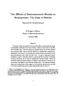
Figures 1-3 show the estimated median impulse response functions of the macroeconomic variables of all individual countries to the three types of oil shocks for the 1986Q1-2010Q4 sample period, together with the 16th and 84th percentile error bands.10 The estimated responses have been accumulated and are shown in levels in the figures. Each oil shock has been normalized to a ten percent long-run increase in the nominal price of oil. To facilitate comparisons, Table 1 also contains the median responses for output and consumer prices at relevant horizons for all countries. Figure 1 illustrates that the economic consequences of an oil supply shock are very different for oil-importing and oil-exporting countries. Consider real GDP in the first column. All net energy-importing countries (France, Italy, US, Japan and Switzerland) experience a permanent fall in economic activity in the long-run, except Spain and Germany, where the long-run impact turns out to be neutral. In contrast, output permanently increases in Norway and Canada, two countries that export both oil and other forms of energy. Despite being a net oil-importing country, real GDP in Australia rises in the long-run (after a temporary decline in the short-run). Australia, however, is a significant non-oil energy exporting country, which probably compensates for the negative oil price effect. Also the UK, who is an oil-exporting but non-oil energy-importing country, experiences 10
The impulse responses of oil production and oil prices are shown in Figure 5 (Section 3.1 of the paper),
when we discuss the changes in oil market dynamics over time.
10
only a transitory fall in economic activity. Overall, not only the role of oil but also other forms of energy in the economy are important to determine the dynamic effects of oil supply shocks on output. This also seems to be the case for the inflationary consequences.11 We find an impact on consumer prices which is relatively strong for all energy-importing countries, except for Spain, whereas inflationary pressures are negligible or even negative in net energy-exporting countries. These different consumer price responses are probably driven by the response of the exchange rate. The exchange rate tends to appreciate in oil-exporting countries, which likely limits the pass-through to inflation.12 The interest rate response after oil supply shocks is generally in accordance with the effect on inflation, i.e. only in oil-importing countries, monetary policy is significantly tightened to stabilize inflation. The economic effects of an oil demand shock driven by global economic activity are substantially different from the impact of exogenous oil supply shocks. Figure 2 shows that all countries experience significant long-run inflationary effects and even a significant short-run increase of real GDP. When we compare the magnitudes across countries in Table 1, the temporary increase of output is similar for all countries, irrespective of the relevance of energy products. Although in contrast with the results after oil supply shocks, this finding is not surprising since we consider an oil price shift that is driven endogenously by a shift in worldwide economic activity. Accordingly, other factors are likely to determine the final effects on economic activity and inflation, rather than the oil and energy intensity of the economy. Output can rise because the country itself is in a boom, or because it indirectly gains from trade with the rest of the world. Also inflation differences are small between most countries. We only observe a stronger impact in Spain and UK. Somewhat surprising, output in UK and Canada declines in the long run. In all countries, the interest rate temporarily increases. The dynamic effects of oil-specific demand shocks are also considerably different compared to the two other sources of oil price shifts, as can be seen in Figure 3. In most of 11
This finding is rather surprising given that PVR (2009) show that, in contrast to the oil intensity of
the economy, asymmetries in labor market characteristics are crucial to explain differences of the impact of oil supply shocks on consumer prices in individual Euro area countries. However, they only consider a set of net oil-importing countries, while we show that differences in oil and energy import dependence do seem to matter when also oil and energy-exporting countries are included in the analysis. 12 For instance, when we add respectively the import and GDP deflator to the Norwegian VAR as an eighth variable, the import deflator considerably falls and the GDP deflator strongly increases after an oil supply shock, which confirms this conjecture.
11
the countries, this shock is characterized by a temporary fall in real GDP with the peak mostly within the first two years after the shock. The effects on consumer prices are on average much smaller compared to other types of oil shocks, and in the long run only significantly positive in the US. In the oil and energy-exporting countries, the exchange rate does not significantly respond, in contrast to the appreciations after an oil supply shock. Comparing cross-country differences of the magnitudes of the effects (see Table 1) indicates that oil-importing and oil-exporting countries react in a similar way, i.e. also after this type of oil demand shock, the role of oil and energy in the economy seems not to matter much. Except for the US and Italy, the interest rate response is generally in line with the reaction of consumer prices. In sum, the underlying source of the oil price increase is crucial to determine the repercussions of oil shocks on the economy. In addition, the role of oil and other forms of energy, i.e. being a net energy-importing or energy-exporting country, is only important to understand the cross-country divergences after exogenous oil supply shocks. These marked differences are absent for shocks at the demand side of the global oil market. Accordingly, making cross-country comparisons solely based on average oil price shocks is misleading since oil prices are determined by a combination of supply and demand disturbances, with each shock affecting the economies differently. In the end, variance decompositions show that for the period 1986-2010, oil supply shocks contribute 40 percent to oil price variability, whilst the contemporaneous contribution of oil demand shocks driven by economic activity and oil-specific demand shocks are respectively 40 and 20 percent.
3
Has the impact changed over time?
3.1
The normalization problem
The way the economy experiences oil shocks appears to have changed fundamentally over time. For the US economy, Mork (1989), Hooker (1996), Bernanke et al. (1997), Herrera and Pesavento (2007), Mila (2009), and Blanchard and Gali (2010) find a reduced impact of oil price shocks on real GDP and inflation in more recent periods, and several of these studies refer to a decreased dependency on crude oil as a possible explanation.13 However, 13
Other structural changes in the economy that have been put forward as an explanation for a reduced
impact of oil shocks over time are improved monetary policy, more flexible labor markets, and changes
12
the oil market itself has also undergone substantial changes. More precisely, Krichene (2002), Ryan and Plourde (2002), Cooper (2003) and BP (2008) find evidence of a lower price elasticity of oil demand since the mid 1980s, whereas Kilian (2008), Hamilton (2009) and BP (2010) find support for a declining oil supply elasticity over time.14 As demonstrated by BP (2008), these changes in the oil market seriously complicate comparisons of the effects of oil shocks over time. For instance, if a comparison of the consequences of an oil supply shock is based on a similar change of crude oil prices (e.g. a 10 percent rise), BP (2008) find a more muted impact on the US economy in more recent periods, which is consistent with the evidence in the oil literature described above. However, such a comparison implicitly assumes a constant price elasticity of oil demand, which is rejected by the data. In particular, normalizing on a certain oil price increase assumes totally different associated oil supply shifts as the price elasticity of demand has lowered over time, i.e. large supply shifts in the 1970s and more limited ones since the second part of the 1980s. Panel A of Figure 4 illustrates this point graphically. For exactly the same reason, normalizing on oil production is also misleading, since a similar shift in oil production currently has a greater impact on oil prices relative to earlier periods, which distorts the comparison. Indeed, BP (2008) find much stronger effects on real GDP and consumer prices in the US in more recent times compared to the 1970s and early 1980s if an exogenous oil supply shock is measured as an oil production shortfall of 1 percent, which contrasts with the normalization on oil prices. Since also the oil supply curve became less elastic over time, this problem of comparability after oil supply shocks also carries over to shocks at the demand side of the oil market, as illustrated in panel B of Figure 4. In Figure 5, we demonstrate this normalization problem in the context of our analyin the importance of the automobile sector (Blanchard and Gali 2010). On the other hand, Lee, Ni and Ratti (1995) and Ferderer (1996) argue that increased oil market volatility has led to a breakdown of the empirical relationship between oil prices and economic activity. These alternative explanations are out of the scope of this paper, but could be explored in future research. 14 The steepening of the oil demand and supply curves can be explained by several factors. A popular explanation of the decreased responsiveness of oil production to price changes is the fact that oil production has been very close to full capacity since the second half of the eighties, leaving no room to increase oil production following oil price shifts. On the other hand, rising oil prices during the 1970s are often seen as a trigger for a reduction in the price elasticity of oil demand afterwards since it induced an increased use of alternative sources of energy, more energy-efficient technologies and improved energy conservation. This created a reduced scope for additional substitution away from oil, which in turn implies a lower price-elasticity of oil demand. For a more comprehensive discussion and additional explanations, we refer to BP (2008 and 2010).
13
sis. BP (2010) model time variation by estimating a Bayesian VAR with time-varying parameters and stochastic volatility. We reproduce their results by estimating the effects for two different sample periods, i.e. 1971Q1-1985Q4 (henceforth ’the seventies’) and 1986Q1-2010Q4 (henceforth ’the nineties’). The latter period is also the one used for the estimations in section 2. The first two columns of panel A show the impulse responses for respectively global oil production and the oil price for one standard deviation shocks. A typical unfavorable oil supply shock in the nineties is characterized by a much smaller fall of world oil production and a greater effect on the price of crude oil relative to the seventies. The corresponding estimated oil demand elasticity can be found in the last column of panel A, and confirms the considerable decline over time. To illustrate the implications for making comparisons over time, panel B shows the impact on US real GDP for an oil supply shock measured respectively as a one standard deviation shock, an oil price increase of 10 percent and an oil production shortfall of 1 percent.15 An oil supply shock that raises oil prices by 10 percent indeed has a smaller impact on activity in the more recent period. However, the effects of a 1 percent innovation in oil production are stronger in the nineties, whereas the impact is more or less constant over time for a one standard deviation shock. Similar difficulties emerge for both oil demand shocks. Whilst the impact of a one standard deviation shock on oil prices did not change a lot, the underlying innovations to oil production are much smaller in the nineties. The corresponding lower price elasticity of oil supply is shown in panel A of Figure 5, whereas the distorted normalization experiment for US real GDP can be found in the bottom two rows of panel B.16 In sum, the normalization problem seriously complicates comparisons of the dynamic effects of oil shocks over time, as normalizing on a specific change in oil prices or production gives misleading results, which makes it difficult to analyze the factors that are important in understanding time-varying effects of oil shocks. In the next section, we propose an approach to avoid this problem. 15
The results for other countries and variables are available upon request, but the consequences are
identical since all countries are subject to the same changes in the global oil market. 16 Note that, since the impact on production in the seventies is only transitory, we had to normalize the effects for a contemporaneous 1 percent decline in oil production.
14
3.2
Structural changes and cross-country differences over time
In order to better understand time variation in the effects of oil shocks, we can explore the cross-country dimension of our analysis. Specifically, we can investigate whether a changing role of oil and energy matters for time variation by comparing the time-varying effects of oil shocks to changes in oil and non-oil energy intensities over time. If a reduced dependency on crude oil and other forms of energy has resulted in a more subdued responsiveness to oil shocks, the change over time should be larger for countries that improved their net energy position or oil intensity the most. Since all countries have been subject to the same structural changes in the oil market, comparing relative changes between countries avoids the normalization problem. Panel A of Table 2 lists several indicators of the country-specific role of oil, non-oil energy and total energy for the 1970-1985 and 1986-2008 periods and the changes of these indicators over time. Whilst all countries experienced a noticeable fall in total energy intensity and an improvement in net oil and energy import dependence, except for Spain, the cross-country differences are substantial. In particular, Norway is the only country that has been a net exporter of crude oil over the entire sample. Its exports of crude oil increased to a level more than seven times as high compared to the seventies. In addition, exports of non-oil energy are also four times higher in the nineties. The oil and gas industry in Norway is currently even the largest contributor to GDP. Whereas Canada and the UK were on average oil-importing countries in the seventies, they switched to being net-exporters since the mid-1980s. Canada also succeeded in more than doubling its net exports of other forms of energy. This rise is even larger for Australia, which increased its net export ratio from 87 tonnes per unit of GDP in the seventies to 220 in the period covering the nineties. Even within the group of net energy-importing countries, the changes are very different over time. France, Germany, Italy and Japan significantly reduced their oil dependency to almost half the level of the seventies. Part of this improvement, however, is compensated by increased imports of other forms of energy, except for France. On the other hand, Spain, the US and Switzerland have hardly improved their reliance on oil imports. Noticeable is the evolution of the US. The overall energy intensity of its economy has been reduced the most over time. However, this reduction can be fully attributed to a fall in domestic production. The net energy import dependence of the US has actually not really changed. With a view to evaluate whether a changed role of oil and other forms of energy 15
in the economy matters for the effects of oil shocks, we compare the change in economic impact with the relative improvement in the net oil and energy position over time. Figure 6 depicts the impact on real GDP of the three types of oil shocks, normalized to a 10 percent increase in oil prices, for respectively the 1970-1985 and 1986-2010 periods.17 The degree of reduced responsiveness between both periods, calculated as the difference between the maximum median response of GDP in the seventies and the nineties to each oil shock, are reported in Panel B of Table 2.18 Table 2 shows that the maximum fall in output after an oil supply shock, normalized on a similar oil price increase, has indeed reduced over time for all countries. The degree of improvement, however, is very different. First, consider the countries that are on average net exporters of energy since 1986 in Panel A of Figure 6, i.e. Norway, Canada, Australia and the UK. Whilst the output effects after oil supply shocks were more or less equally severe as in the net energy-importing countries in the seventies, the effects on economic activity became insignificant or even positive in more recent times. These net energy-exporting countries also made considerable advances in their net oil and total energy positions over time (see Panel A of Table 2). Second, among the net energy-importing countries, Japan and Germany experienced the greatest decline in the output effects of oil supply shocks. At the same time, together with France, both countries also improved their net imports of oil and total energy the most over time. Overall, relative improvements in the oil and energy positions could explain the changed effects of oil supply shocks over time.19 In contrast, the role of oil and energy appears not to matter for explaining time variation following shocks at the demand-side of the oil market. For oil demand shock driven by fluctuations in economic activity, this is not surprising given the (non-oil) nature of this shock as discussed in section 2.3. Following an oil-specific demand shock, most netenergy exporting countries managed to reduce the negative economic effects, in contrast to some of the net-energy importing countries (see last column of Table 2). However, also 17
Since we only compare the relative changes over time across countries, it does not matter whether we
normalize on oil prices or oil production. 18 Note that if we would consider the change in the long-run impact on economic activity instead of the difference in the maximum effect, we would not take into account that in several countries also the shape of the response has changed considerably. This is clearly the case for Japan and Switzerland after an oil supply shock for example. 19 Rank correlations of 0.75 and 0.49 between the change in output effects and respectively the change in net energy and net oil imports over time confirm that the time-varying effects of oil supply shocks can be related to the changes in oil and energy dependence.
16
no clear connection can be found between the reduction in oil and energy dependence and the change in real effects following this demand-side shock. In sum, these results support the hypothesis that the oil and non-oil energy intensities are important to explain cross-country differences over time, but after oil supply shocks only.
4
Conclusions
In this paper, we compared the dynamic effects of several types of oil shocks across a set of industrialized countries which are very diverse with respect to the role of oil and other forms of energy in their economy. Several important insights emerge from this analysis. First, the underlying source of the oil price shift is crucial to determine the macroeconomic consequences in each country, which is in line with the results of Kilian (2009) and Peersman and Van Robays (2009) for the United States and Euro area respectively. More specifically, for oil demand shocks that are driven by shifts in global economic activity, all countries experience a temporary increase of economic activity and a significant rise in inflation. Conversely, oil-specific demand shocks are mostly followed by a transitory decline of output and negligible inflationary effects. The role of oil and energy does not seem relevant for explaining cross-country differences in the impact of both demand shocks. This role, however, is very important to determine the economic effects of exogenous oil supply shocks. In particular, all net oil and energy-importing countries are confronted with a fall in economic activity and a rise of inflation. On the other hand, the long-run impact on real GDP is insignificant or even positive in countries that are net energy-exporters. In addition, also the impact on inflation is much more subdued, probably driven by an appreciation of the exchange rate in this group of countries. As a result, not disentangling oil price shocks based on their underlying source could seriously bias estimations of the cross-country effects of oil shocks. Second, making a comparison of the dynamic effects of oil shocks over time implicitly poses a normalization problem, since both oil demand and supply have become less price elastic since the mid-1980s. Considering the time-varying impact of a certain oil price increase, or alternatively a specific fall in oil production, implies a bias since totally different associated oil shocks are assumed. We showed that by using the cross-country dimension and considering relative changes over time, we can avoid this normalization problem. In particular, if the role and share of oil and energy is important for understanding time
17
variation, the change in the effects should be more favorable for countries that improved their oil and energy position the most over time. Our results show that the degree of improvement in oil and energy dependence is indeed important for time-variation in the effects of oil supply shocks and for explaining the associated cross-country differences. Our evidence obviously does not exclude that other factors are also relevant determinants for cross-country differences in the economic repercussions and time-varying effects of oil shocks. Whereas we have only analyzed the role of oil and energy, also monetary policy credibility, labor market characteristics or other structural features could matter to explain asymmetries. The relevance of other determinants is something which could be explored in future research, in particular for the effects on inflation. A first attempt for individual Euro area countries has been made by Peersman and Van Robays (2009).
18
References [1] Baumeister, C. and G. Peersman (2008), "Time-Varying Effects of Oil Supply Shocks on the US Economy", Ghent University Working Paper 2008/515. [2] Baumeister, C. and G. Peersman (2010), "Sources of the Volatility Puzzle in the Crude Oil Market", Ghent University Working Paper 2010/634. [3] Bauwens, L., Lubrano, M. and J-F. Richard (1999), Bayesian Inference in Dynamic Econometric Models, Oxford University Press. [4] Bernanke, B., M. Gertler and M. Watson, (1997), “Systematic Monetary Policy and the Effects of Oil Shocks", Brookings Papers on Economic Activity, 1997-1, p 91-157. [5] Blanchard, O.J. and J. Galí (2010), "The Macroeconomic Effects of Oil Price Shocks: Why Are the 2000s so Different from the 1970s?", Gali J. and M.J. Gertler (eds.), International Dimensions of Monetary Policy, National Bureau of Economic Research, p 373-420. [6] Bruno, M. and J. Sachs (1985), Economics of Worldwide Stagflation, Harvard University Press, Cambridge Massachusetts. [7] Burbidge, J. and A. Harrison (1984), "Testing for the Effects of Oil-Price Rises Using Vector Autoregressions", International Economic Review, 25(2), p 459-484. [8] Cologni, A. and Manera, M. (2008),”Oil Prices, Inflation and Interest Rates in a Structural Cointegrated VAR Model for the G-7 Countries,” Energy Economics, 30(3), p 856-888. [9] Cooper, J.C.B. (2003), "Price Elasticity of Demand for Crude Oil: Estimates for 23 Countries", OPEC Review, 27(1), p 1-8. [10] Cuñado, J. and F. Péres de Gracia (2003), "Do Oil Price Shocks Matter? Evidence for some European Countries", Energy Economics, 25, p 137-154. [11] Darby, M. (1982), "The Price of Oil and World Inflation and Recession", American Economic Review, 72, p 738-751. [12] Ferderer, J.P. (1996), "Oil Price Volatility and the Macroeconomy", Journal of Macroeconomics, 18(1), p 1-26. 19
[13] Geweke, J. (2005), Contemporary Bayesian Econometrics and Statistics, John Wiley & Sons, Inc. [14] Hamilton, J.D. (1983), "Oil and the Macroeconomy Since World War II", Journal of Political Economy, 91(2), p 228-248. [15] Hamilton, J.D. (2003), "What is an Oil Shock?", Journal of Econometrics, 113, p 363-398. [16] Hamilton, J.D. (2009), "Causes and Consequences of the Oil Shock of 2007-2008", Brookings Papers on Economic Activity, Spring, p 215-259. [17] Herrera, A.M. and E. Pesavento (2007), "Oil Price Shocks, Systematic Monetary Policy and the ‘Great Moderation’", Macroeconomic Dynamics, 13(1), p 107-137. [18] Hooker, M.A. (1996), "What Happened to the Oil Price—Macroeconomy Relationship?", Journal of Monetary Economics, 38(October), p 195-213. [19] Hubbard, R.G. (1986), "Supply Shocks and Price Adjustment in the World Oil Market", Quarterly Journal of Economics, 101(1), p 85-102. [20] Jimenez-Rodriguez, R. (2008), “The Impact of Oil Price Shocks: Evidence from the Industries of Six OECD Countries,” Energy Economics, 30(6), p 3095-3108. [21] Jiménez-Rodríguez, R. and M. Sánchez (2005), "Oil Price Shocks and Real GDP Growth: Empirical Evidence for Some OECD Countries", Applied Economics, 37(2), p 201-228. [22] Kilian, L. (2008), "A Comparison of the Effects of Exogenous Oil Supply Shocks on Output and Inflation in the G7 Countries", Journal of the European Economic Association, 6(1), p 78-121. [23] Kilian, L. (2009), "Not All Oil Price Shocks Are Alike: Disentangling Demand and Supply Shocks in the Crude Oil Market", American Economic Review, 99(3), June 2009. [24] Korhonen, I. and S. Ledyaeva (2010) “Trade Linkages and Macroeconomic Effects of the Price of Oil,” Energy Economics, 32(4), p 848-856.
20
[25] Krichene, N. (2002), "World Crude Oil and Natural Gas: A Demand and Supply Model", Energy Economics, 24, p 557-576. [26] Lancaster, T. (2004), Introduction to Modern Bayesian Econometrics, Blackwell Publishing Ltd. [27] Lardic, S. and V. Mignon (2008), “Oil Prices and Economic Activity: An Asymmetric Cointegration Approach”, Energy Economics, 30(3), p 847-855. [28] Lee, K., S. Ni, and R.A. Ratti (1995), "Oil Shocks and the Macroeconomy: The Role of Price Variability", The Energy Journal, 16(4), p 39-56. [29] Lee, K. and S. Ni (2002), “On the Dynamic Effects of Oil Price Shocks: a Study Using Industry Level Data”, Journal of Monetary Economics, 49, p 823—852. [30] Lombardi, M. and I. Van Robays (2011), "Do Financial Investors Destabilize the Oil Price?", Working Paper Series, European Central Bank, 1346. [31] Mila, F. (2009), “Expectations, Learning, and the Changing Relationship between Oil Prices and the Macroeconomy,” Energy Economics, 31(6), p 827-837. [32] Mork, K. (1989), "Oil and the Macroeconomy When Prices Go Up and Down: An Extension of Hamilton’s Results", Journal of Political Economy, 97(3), p 740-744. [33] Mork, P., O. Oslen and H. Mysen (1994), "Macroeconomic Responses to Oil Price Increases and Decreases in Seven OECD Countries", The Energy Journal, 15, p 15-38. [34] Papapetrou, E. (2001), “Oil Price Shocks, Stock Market, Economic Activity and Employment in Greece”, Energy Economics, 23, p 511-532. [35] Paustian, M. (2007), "Assessing Sign Restrictions", The B.E. Journal of Macroeconomics, 7(1), Article 23. [36] Peersman, G. (2005), "What Caused the Early Millennium Slowdown? Evidence Based on Vector Autoregressions", Journal of Applied Econometrics, 20, p 185-207. [37] Peersman, G. and I. Van Robays (2009), "Oil and the Euro Area Economy", Economic Policy, 24(60), p 603-651.
21
[38] Rotemberg, J.J. (2010), "Comment on Blanchard-Galí: The Macroeconomic Effects of Oil Price Shocks: Why are the 2000s so Different from the 1970s", Gali J. and M.J. Gertler (eds.), International Dimensions of Monetary Policy, National Bureau of Economic Research, p 421-428. [39] Rasche, R. H., and J. A. Tatom (1977), "Energy Resources and Potential GNP," Federal Reserve Bank of St. Louis Review, 59, p 10-24. [40] Rasche, R. H., and J. A. Tatom (1981), "Energy Price Shocks, Aggregate Supply, and Monetary Policy: The Theory and International Evidence", Brunner K. and A. H. Meltzer (eds.), Supply Shocks, Incentives, and National Wealth, Carnegie-Rochester Conference Series on Public Policy, vol. 14, Amsterdam: North-Holland. [41] Ryan, D.L. and A. Plourde (2002), "Smaller and Smaller? The Price Responsiveness of Nontransport Oil Demand", Quarterly Review of Economics and Finance, 42, p 285-317. [42] Sims, C. A. and T. Zha (1999), “Error Bands for Impulse Responses", Econometrica, 67(5), p 1113-1155. [43] Zellner, A. (1996), An Introduction to Bayesian Inference in Econometrics, Wiley Classics Library, John Wiley & Sons, Inc.
22
Real GDP
Consumer prices
0,7
Interest rate
1,0
Exchange rate
0,6
3,0
0,4
2,0
0,2
1,0
0,5 0,6
United States
0,3 0,1
0,2
-0,1 -0,3 -0,5
0,0
0,0
-0,2
-1,0
-0,4
-2,0
-0,2
-0,7 -0,9
-0,6
-1,1 -1,3 0
4
8
12
16
20
24
28
0
4
8
12
16
20
24
0
28
1,0
0,7
-3,0
-0,6
-1,0
4
8
12
16
20
24
28
0,6
3,0
0,4
2,0
0,2
1,0
0
4
8
12
16
20
24
28
0
4
8
12
16
20
24
28
0
4
8
12
16
20
24
28
0
4
8
12
16
20
24
28
0
4
8
12
16
20
24
28
0,5 0,6
0,3
Japan
0,1 0,2
-0,1 -0,3
0,0
0,0
-0,2
-1,0
-0,4
-2,0
-0,2
-0,5 -0,7
-0,6
-0,9 -1,1
-1,0
-1,3 0
4
8
12
16
20
24
-0,6 0
28
0,7
4
8
12
16
20
24
28
1,0
-3,0 0
4
8
12
16
20
24
28
0,6
3,0
0,4
2,0
0,2
1,0
0,5
Switzerland
0,3
0,6
0,1 -0,1
0,2
-0,3 -0,5
0,0
0,0
-0,2
-1,0
-0,4
-2,0
-0,2
-0,7 -0,9
-0,6
-1,1 -1,3
-1,0 0
4
8
12
16
20
24
28
0,7
-3,0
-0,6 0
4
8
12
16
20
24
28
1,0
0
4
8
12
16
20
24
28
0,6
3,0
0,4
2,0
0,2
1,0
0,5 0,3
0,6
France
0,1 -0,1
0,2 0,0
0,0
-0,2
-1,0
-0,6
-0,4
-2,0
-1,0
-0,6
-0,3 -0,5
-0,2
-0,7 -0,9 -1,1 -1,3 0
4
8
12
16
20
24
28
0,7
0
4
8
12
16
20
24
1,0
-3,0 0
28
4
8
12
16
20
24
28
0,6
3,0
0,4
2,0
0,2
1,0
0,5 0,6
0,3
Germany
0,1 0,2
-0,1
0,0
0,0
-0,3 -0,5
-0,2
-1,0
-0,2
-0,7 -0,9
-0,6
-2,0
-0,4
-1,1 -3,0 -1,3
-0,6
-1,0 0
4
8
12
16
20
24
28
0
4
8
12
16
20
24
1,0
0,7
0
28
4
8
12
16
20
24
28
0,6
3,0
0,4
2,0
0,2
1,0
0,0
0,0
0,5 0,6
0,3 0,1
0,2
Italy
-0,1 -0,3
-0,2
-0,5
-0,2
-1,0
-0,6
-0,4
-2,0
-1,0
-0,6
-0,7 -0,9 -1,1 -1,3 0
4
8
12
16
20
24
0
28
0,7
4
8
12
16
20
24
1,0
-3,0 0
28
4
8
12
16
20
24
0
28
0,6
3,0
0,4
2,0
0,2
1,0
4
8
12
16
20
24
28
0,5 0,3
0,6
Spain
0,1 -0,1
0,2
-0,3 -0,5
0,0
0,0
-0,2
-1,0
-0,2
-0,7 -0,9
-0,6
-0,4
-2,0
-1,1 -1,3
-1,0 0
4
8
12
16
20
24
28
-0,6 0
4
8
00 2 6 11 0 20 6
12
16
20
24
28
-3,0 0
4
8
12
16
20
24
28
0
4
8
12
16
20
24
28
05 1 2
Figure 1. Impact of oil supply shock Notes: Figures are median impulse responses to a 10 percent long-run rise in oil prices, together with the 16th and 84th percentile error bands, horizon is quarterly.
Real GDP
Consumer prices
0,7
Interest rate
1,0
Exchange rate
0,6
3,0
0,4
2,0
0,2
1,0
United kingdom
0,5 0,3
0,6
0,1 -0,1
0,2
-0,3 -0,5
0,0
0,0
-0,2
-1,0
-0,4
-2,0
-0,2
-0,7 -0,9
-0,6
-1,1 -1,3
-0,6
-1,0 0
4
8
12
16
20
24
28
0
4
8
12
16
20
24
1,0
0,7
-3,0 0
28
4
8
12
16
20
24
28
0,6
3,0
0,4
2,0
0,2
1,0
0
4
8
12
16
20
24
28
0
4
8
12
16
20
24
28
0
4
8
12
16
20
24
28
0
4
8
12
16
20
24
28
0,5 0,3
0,6
Canada
0,1 -0,1
0,2
-0,3 -0,5
0,0
0,0
-0,2
-1,0
-0,4
-2,0
-0,2
-0,7 -0,9
-0,6
-1,1 -1,3
-0,6
-1,0 0
4
8
12
16
20
24
28
0
4
8
12
16
20
24
1,0
0,7
-3,0 0
28
4
8
12
16
20
24
28
0,6
3,0
0,4
2,0
0,2
1,0
0,5 0,6
0,3
Australia
0,1 0,2
-0,1 -0,3
0,0
0,0
-0,2
-1,0
-0,4
-2,0
-0,2
-0,5 -0,7
-0,6
-0,9 -1,1
-1,0
-1,3 0
4
8
12
16
20
24
-0,6 0
28
4
8
12
16
20
24
28
1,0
0,7
-3,0 0
4
8
12
16
20
24
28
0,6
3,0
0,4
2,0
0,2
1,0
0,5 0,3
0,6
Norway
0,1 -0,1
0,2
-0,3 -0,5
0,0
0,0
-0,2
-1,0
-0,4
-2,0
-0,2
-0,7 -0,9
-0,6
-1,1 -1,3
-1,0 0
4
8
12
16
20
24
28
-3,0
-0,6 0
4
8
12
16
20
24
28
0
4
8
12
16
20
24
28
Figure 1 continued. Impact of oil supply shock Notes: Figures are median impulse responses to a 10 percent long-run rise in oil prices, together with the 16th and 84th percentile error bands, horizon is quarterly.
Real GDP
Consumer prices
Interest rate
1,8
1,0
Exchange rate 4,0
0,7
1,6
United States
0,5
3,0
0,5
1,4
2,0 1,2 0,0
0,3 1,0
1,0 0,1 0,8
0,0
-0,5 0,6
-0,1 -1,0
0,4
-1,0
-0,3
-2,0
0,2 -1,5
0,0 0
4
8
12
-0,5
16
0
4
8
12
16
20
24
-3,0
28
0
4
8
12
16
20
24
28
0
4
8
12
16
20
24
28
0
4
8
12
16
20
24
28
0
4
8
12
16
20
24
28
0
4
8
12
16
20
24
28
0
4
8
12
16
20
24
28
8
12
16
20
24
28
12
16
20
24
28
00 1,0
1,8
4,0
0,7
1,6
3,0
0,5
0,5
1,4 2,0
Japan
1,2
0,3
0,0
1,0
1,0 0,1 0,8
-0,5
0,0 -0,1
0,6
-1,0 0,4
-1,0
-0,3
-2,0
0,2 -1,5 0
4
8
12
16
-0,5
0,0 0
4
8
12
16
20
24
-3,0 0
28
4
8
12
16
20
24
28
0,7
1,6 0,5
Switzerland
4,0
1,8
1,0
3,0
0,5
1,4
2,0 0,3
1,2
1,0
0,0 1,0
0,1 0,0
0,8 -0,5 -0,1
0,6
-1,0
0,4
-1,0
-0,3
-2,0
0,2 0,0
-1,5 0
4
8
12
0
16
1,0
-0,5 4
8
12
16
20
24
28
1,8
-3,0 0
4
8
12
16
20
24
28
4,0
0,7
1,6
3,0
0,5
0,5
1,4 2,0
France
1,2
0,3
0,0
1,0
1,0 0,1
0,8
-0,5
0,0 -0,1
0,6
-1,0
0,4
-1,0
-0,3
-2,0
0,2
-1,5 0
4
8
12
16
0
4
8
12
16
20
24
0
28
1,8
1,0
-3,0
-0,5
0,0
4
8
12
16
20
24
28
4,0
0,7
1,6
3,0
0,5
0,5
1,4
Germany
2,0 1,2
0,3
0,0
1,0
1,0 0,1 0,8
0,0
-0,5 -0,1
0,6
-1,0 0,4
-1,0
-0,3
-2,0
0,2 -1,5
-0,5
0,0 0
4
8
12
16
0
4
8
12
16
20
24
-3,0 0
28
4
8
12
16
20
24
28
00 1,8
1,0
4,0
0,7
1,6
3,0
0,5
0,5
1,4 2,0 1,2
0,3
Italy
0,0
1,0
1,0 0,1 0,8
-0,5
0,0 -0,1
0,6
-1,0 0,4
-1,0
-0,3
-2,0
0,2 -1,5 0
4
8
12
16
-0,5
0,0 0
4
8
12
16
20
24
-3,0 0
28
4
8
12
16
20
24
28
0,7 1,0
4
1,8 1,6
0,5
3,0
0,5
1,4
2,0 0,3
1,2
Spain
0
4,0
0,0
1,0 1,0
0,1 0,0
0,8 -0,5 -0,1
0,6
-1,0
0,4
-1,0
-0,3
-2,0
0,2 -1,5
0,0 0
4
8
12
16
-0,5 0
4
8
12
16
20
24
28
-3,0 0
4
8
12
16
20
24
28
0
4
8
Figure 2. Impact of oil demand shock driven by economic activity Notes: Figures are median impulse responses to a 10 percent long-run rise in oil prices, together with the 16th and 84th percentile error bands, horizon is quarterly.
Real GDP
Consumer prices
1,0
Interest rate
1,8
Exchange rate 4,0
0,7
United kingdom
1,6
3,0
0,5
0,5
1,4 2,0 0,3
1,2
0,0
1,0
1,0 0,1
0,8
0,0
-0,5 -0,1
0,6
-1,0
0,4
-1,0
-0,3
-2,0
0,2
-1,5 0
4
8
12
16
0
4
8
12
16
20
24
0
28
1,8
1,0
-3,0
-0,5
0,0
4
8
12
16
20
24
28
0,7
4,0
0,5
3,0
1,6 0,5
0
4
8
12
16
20
24
28
0
4
8
12
16
20
24
28
0
4
8
12
16
20
24
28
0
4
8
12
1,4 2,0 0,3
Canada
1,2 0,0
1,0
1,0 0,1 0,8
0,0
-0,5 -0,1
0,6
-1,0 0,4
-1,0
-0,3
-2,0
0,2 0,0
-1,5 0
4
8
12
1,0
-3,0
-0,5 0
16
4
8
12
16
20
24
28
1,8
0
4
8
12
16
20
24
28
4,0
0,7
1,6
3,0
0,5
0,5
1,4
Australia
2,0 1,2
0,3
0,0
1,0
1,0 0,1 0,8
0,0
-0,5 0,6
-0,1 -1,0
0,4
-1,0
-0,3
-2,0
0,2 -1,5
0,0 0
4
8
12
16
0
4
8
12
16
20
24
28
1,8
1,0
-3,0
-0,5 0
4
8
12
16
20
24
28
4,0
0,7
1,6
3,0
0,5
0,5
1,4 2,0
Norway
1,2
0,3
0,0
1,0
1,0 0,1 0,8
0,0
-0,5 0,6
-0,1 -1,0
0,4
-1,0
-0,3
-2,0
0,2 -1,5
0,0 0
4
8
12
16
-0,5 0
4
8
12
16
20
24
28
-3,0 0
4
8
12
16
20
24
28
16
20
24
28
Figure 2 continued. Impact of oil demand shock driven by economic activity Notes: Figures are median impulse responses to a 10 percent long-run rise in oil prices, together with the 16th and 84th percentile error bands, horizon is quarterly.
United States
Real GDP
Consumer prices
1,0
2,5
0,5
2,0
-1,0
-2,0
0,0 -0,8
-1,5
-3,5
-0,5 -2,0
-1,0
-5,0
-1,3
-6,5
-1,5 -2,0 4
8
12
1,0
2,5
0,5
2,0
-8,0
-1,8 0
16
4
8
12
16
20
24
28
0
4
8
12
16
20
24
28
0
4
8
12
16
20
24
28
0
4
8
12
16
20
24
28
0
4
8
12
16
20
24
28
0
4
8
12
16
20
24
28
0
4
8
12
16
20
24
28
0
4
8
12
16
20
24
28
0
4
8
12
16
20
24
28
0,7 4,0
1,5
2,5
0,2
1,0
1,0
-0,5
Japan
1,0 -0,5
-0,3
0,5
0,0
-0,3
0,5
-0,5
-1,0 -2,0
0,0 -0,8
-1,5
-3,5
-0,5 -2,0
-1,0
-2,5
-5,0
-1,3
-6,5
-1,5
-3,0
-2,0 0
4
8
12
-1,8
16
0
1,0
2,5
0,5
2,0
4
8
12
16
20
24
-8,0
28
0
4
8
12
16
20
24
28
0,7 4,0
1,5
0,0
Switzerland
2,5
1,0
0
2,5
0,2
1,0
1,0 -0,5
-0,5
-0,3
0,5 -1,0
-2,0
0,0 -0,8
-1,5
-3,5
-0,5 -2,0
-5,0
-1,0
-2,5
-1,3 -6,5
-1,5
-3,0
-2,0 0
4
8
12
16
2,5
0,5
2,0
0,0
1,5
-8,0
-1,8 0
1,0
4
8
12
16
20
24
28
0
4
8
12
16
20
24
28
0,7
4,0 2,5
0,2
1,0
1,0
-0,5
France
4,0
0,2
-0,5
-3,0
-0,3
0,5
-0,5
-1,0 -2,0
0,0 -0,8
-1,5
-3,5
-0,5 -2,0
-1,0
-2,5
-5,0
-1,3
-6,5
-1,5
-3,0 0
4
8
12
16
-1,8
-2,0 0
1,0
2,5
0,5
2,0
4
8
12
16
20
24
0
28
4
8
12
16
20
24
28
-8,0
0,7 4,0
1,5
0,0
Germany
Exchange rate
0,7
1,5
0,0
-2,5
2,5
0,2
1,0
1,0 -0,5
-0,5
-0,3
0,5 -1,0
-2,0
0,0 -0,8
-1,5
-3,5
-0,5 -2,0
-1,0
-2,5
-5,0
-1,3
-6,5
-1,5
-3,0
-2,0 0
4
8
12
1,0
2,5
0,5
2,0
-8,0
-1,8 0
16
4
8
12
16
20
24
28
0
4
8
12
16
20
24
28
0,7 4,0
1,5
0,0
2,5
0,2
1,0
1,0
-0,5
Italy
Interest rate
-0,3
0,5
-0,5
-1,0 -2,0
0,0 -0,8
-1,5
-3,5
-0,5 -2,0
-1,0
-2,5
-5,0
-1,3
-1,5
-3,0
-6,5
-2,0 0
4
8
12
16
-1,8 0
1,0
2,5
0,5
2,0
4
8
12
16
20
24
28
-8,0 0
4
8
12
16
20
24
28
0,7 4,0
1,5
0,0
2,5
0,2
1,0
1,0
Spain
-0,5 -0,3
0,5
-0,5
-1,0 -2,0
0,0 -0,8
-1,5
-3,5
-0,5 -2,0
-1,0
-2,5
-5,0
-1,3
-6,5
-1,5
-3,0
-2,0 0
4
8
12
16
-8,0
-1,8 0
4
8
12
16
20
24
20
28
0
4
8
12
16
20
24
28
65 0 1 3 4 0
Figure 3. Impact of oil-specific demand shock Notes: Figures are median impulse responses to a 10 percent long-run rise in oil prices, together with the 16th and 84th percentile error bands, horizon is quarterly.
Real GDP
Consumer prices
Interest rate
Exchange rate
United kingdom
18 1,0
2,5
0,5
2,0
0,0
1,5
1,0 -0,3
0,5
-0,5 -2,0
0,0 -0,8
-1,5
-3,5
-0,5 -2,0
-1,0
-2,5
-5,0
-1,3
-6,5
-1,5 4
8
12
16
-1,8
-2,0 0
1,0
2,5
0,5
2,0
4
8
12
16
20
24
0
28
4
8
12
16
20
24
28
-0,8
16
2,5
0,5
2,0
4
8
12
16
20
24
28
4
8
12
16
20
24
28
-8,0 0
4
8
12
16
20
24
28
0,7 4,0
1,5
0,0
0
-3,5
-1,8 0
1,0
28
-6,5
-2,0 12
24
-1,3
-1,5
8
20
-5,0
-1,0
4
16
-2,0
0,0 -0,5
0
12
1,0
-1,5
-3,0
8
-0,5
-0,3
0,5
-2,5
4
2,5
-1,0
-2,0
0
4,0
0,2
1,0
-0,5
-8,0
0,7
1,5
0,0
Canada
2,5
-1,0
0
Australia
4,0
0,2
1,0
-0,5
-3,0
2,5
0,2
1,0
1,0 -0,5 -0,3
0,5
-0,5
-1,0 -2,0
0,0 -0,8
-1,5
-3,5
-0,5 -2,0
-5,0
-1,0
-2,5
-1,3 -6,5
-1,5
-3,0
-2,0 0
4
8
12
16
2,5
0,5
2,0
-8,0
-1,8 0
1,0
4
8
12
16
20
24
28
0
4
8
12
16
20
24
28
0,7
4
8
12
16
20
24
28
0
4
8
12
16
20
24
28
4,0
0,2 1,0
1,0
-0,5
0
2,5
1,5
0,0
Norway
0,7
-0,5
-0,3
0,5 -1,0
-2,0
0,0 -0,8
-1,5
-3,5
-0,5 -2,0
-1,0
-2,5
-5,0
-1,3
-6,5
-1,5
-3,0
-1,8
-2,0 0
4
8
12
16
0
4
8
12
16
20
24
28
-8,0 0
4
8
12
16
20
24
28
Figure 3 continued. Impact of oil-specific demand shock Notes: Figures are median impulse responses to a 10 percent long-run rise in oil prices, together with the 16th and 84th percentile error bands, horizon is quarterly.
PANEL A: Oil supply shock and a similar oil price increase
1970s
Poil
D
1990s
D
Poil
S2
S2
S1 P2
S1
P1
Q2
Q1
Q2 Q1
Qoil
Qoil
PANEL B: Oil demand shock and a similar oil price increase
1970s
Poil
P2
D2
1990s
D2
Poil
D1
S
D1
S
P1
Q1
Q2
Qoil
Figure 4. Oil price increase and different elasticities of oil demand and supply
Q1 Q2
Qoil
PANEL A. Oil market dynamics over time Oil production (1 stdv)
Oil price (1 stdv)
(∆Qoil/Qoil)/(∆Poil/Poil) 0,0
20,0 1,5
18,0
Oil supply shock
-0,1 16,0 0,5
14,0
-0,2
12,0 -0,5
-0,3
10,0 8,0
-1,5
-0,4 6,0
-2,5
4,0
-0,5
2,0 -3,5
0
4
8
12
16
20
-0,6
0,0
0
4
8
12
16
20
Oil-specific demand shock
Global economic activity shock
20,0 1,5
0
4
8
12
16
20
0
4
8
12
16
20
4
8
12
16
20
0,7
18,0
0,6
16,0 0,5
0,5
14,0 12,0
0,4
10,0
0,3
-0,5 8,0
-1,5
0,2 6,0 0,1
4,0
-2,5
0,0
2,0 0,0
-3,5
0
4
8
12
16
0
20
4
8
12
16
-0,1
20
2,5
20,0 1,5
18,0 2,0
16,0 0,5
14,0
1,5
12,0 -0,5 1,0
10,0 8,0
-1,5
0,5
6,0 4,0
-2,5
0,0
2,0 -3,5
0,0
0
4
8
12
16
-0,5
20
0
4
8
12
16
20
0
PANEL B. Normalisation problem for the US US GDP (1 stdv)
US GDP (10% ∆ Poil)
0,2
US GDP (1% ∆ Qoil)
0,5
0,2
Oil supply shock
0,1 0,0
0,0 -0,1
-0,2 -1,0
-0,3
-0,4
-0,4 -1,5 -0,5
-0,6
-0,6
-2,0
-0,7
-0,9
0
Global economic activity shock
-0,8
-2,5
-0,8
Oil-specific demand shock
0,0
-0,5
-0,2
4
8
12
16
20
1,0
-3,0
-1,0
0
4
8
12
16
20
3,0
0
4
8
12
16
20
0
4
8
12
16
20
0
4
8
12
16
20
5,0
2,0 4,0
0,5
1,0 3,0
0,0 0,0 -1,0
2,0
-2,0
-0,5
1,0
-3,0 -4,0
-1,0
0,0
-5,0
-1,0
-6,0
-1,5
-2,0
-7,0 -2,0
-8,0
0
4
8
12
16
20
0
4
8
12
16
20
1,0
0,4
-3,0
0,2
0,5 0,2
0,0
0,0 -0,5
0,0
-0,2
-1,0 -1,5
-0,2
-0,4
-2,0 -0,4
-0,6
-2,5 -3,0
-0,6
-0,8
-3,5 -4,0
-0,8
0
4
8
12
16
20
0
4
8
12
16
20
-1,0
Figure 5. Oil market dynamics over time and the normalisation problem for the US Notes: Figures are median impulse responses, together with the 16th and 84th percentile error bands, horizon is quarterly, 1971-1985: dotted lines, 1986-2010: full lines. The responses in Panel A are estimated from a VAR model that only contains oil production, the oil price and world industrial production. In Panel B, we normalized the effects on US GDP for a 10 percent long-run increase in oil prices following all oil shocks, a 1 percent long-term increase in oil production following an oil supply shock, and a contemporaneous 1 percent change in oil production following the oil demand shocks.
PANEL A: Effect of oil supply shock on GDP over time United States
Japan
Switzerland
1,0
1,0
1,0
0,5
0,5
0,5
0,0
0,0
0,0
-0,5
-0,5
-0,5
-1,0
-1,0
-1,0
-1,5
-1,5
-1,5
-2,0
-2,0
-2,0
-2,5
-2,5
-3,0 0
4
8
12
16
20
-2,5 -3,0
-3,0 0
4
France
8
12
16
0
20
4
Germany
8
12
16
20
Italy
Spain
1,0
1,0
1,0
1,0
0,5
0,5
0,5
0,5
0,0
0,0
0,0
0,0
-0,5
-0,5
-0,5
-0,5
-1,0
-1,0
-1,0
-1,0
-1,5
-1,5
-1,5
-1,5
-2,0
-2,0
-2,0
-2,0
-2,5
-2,5
-2,5
-3,0 4
8
12
16
20
-2,5
-3,0
-3,0 0
0
4
United Kingdom
8
12
16
-3,0 0
20
4
Canada
8
12
16
20
0
1,0
1,0
1,0
0,5
0,5
0,5
0,5
0,0
0,0
0,0
0,0
-0,5
-0,5
-0,5
-0,5
-1,0
-1,0
-1,0
-1,0
-1,5
-1,5
-1,5
-1,5
-2,0
-2,0
-2,0
-2,0
-2,5
-2,5
-2,5
-3,0 0
4
8
12
16
20
4
8
12
16
20
12
16
20
12
16
20
12
16
20
12
16
20
-2,5 -3,0
-3,0 0
8
Norway
1,0
-3,0
4
Australia
0
4
8
12
16
0
20
4
8
PANEL B: Effect of oil demand shock driven by economic activity on GDP over time United States
Japan
Switzerland
8,0
5,0
5,0
6,0
4,0
4,0
4,0
3,0
3,0
2,0
2,0
1,0
1,0
2,0 0,0
0,0
0,0
-1,0
-1,0
-2,0
-2,0
-2,0 -4,0 -6,0
-3,0
-8,0 0
4
8
12
16
20
-3,0
-4,0
-4,0 0
4
8
12
16
20
0
4
Germany
France
8
12
16
20
Italy
Spain
5,0
5,0
8,0
5,0
4,0
4,0
6,0
4,0
3,0
3,0
2,0
2,0
3,0
4,0
2,0 2,0
1,0
1,0
1,0 0,0
0,0
0,0
-1,0
-1,0
0,0 -2,0
-2,0
-2,0
-3,0
-3,0
-4,0
-1,0 -4,0
4
8
12
16
20
-3,0
-8,0
-4,0 0
-2,0
-6,0
0
4
United Kingdom
8
12
16
-4,0 0
20
4
Canada
8
12
16
20
0
5,0
5,0
5,0
4,0
4,0
4,0
4,0
3,0
3,0
3,0
3,0
2,0
2,0
2,0
2,0
1,0
1,0
1,0
1,0
0,0
0,0
0,0
0,0
-1,0
-1,0
-1,0
-1,0
-2,0
-2,0
-2,0
-2,0
-3,0
-3,0
-3,0
-4,0 0
4
8
12
16
20
-3,0 -4,0
-4,0 0
4
8
12
16
20
8
Norway
5,0
-4,0
4
Australia
0
4
8
12
16
20
0
4
8
Figure 6. The effects of different types of oil shocks on GDP over time Notes: The figures are median impulse response function to a 10 percent long-run increase in oil prices, together with the 16th and 84th percentile error bands, horizon is in quarters, 1971-1985: dotted lines, 1986-2010: full lines.
PANEL C: Effect of oil-specific demand shock on GDP over time United States
Japan
Switzerland
3,0
3,0
3,0
2,0
2,0
2,0
1,0
1,0
1,0
0,0
0,0
0,0
-1,0
-1,0
-1,0
-2,0
-2,0
-2,0
-3,0 0
4
8
12
16
20
-3,0
-3,0 0
4
France
8
12
16
20
0
4
Germany
8
12
16
20
Italy
Spain
3,0
3,0
3,0
3,0
2,0
2,0
2,0
2,0
1,0
1,0
1,0
1,0
0,0
0,0
0,0
0,0
-1,0
-1,0
-1,0
-1,0
-2,0
-2,0
-2,0
-2,0
-3,0
-3,0
-3,0
0
4
8
12
16
20
0
4
United Kingdom
8
12
16
-3,0 0
20
4
Canada
8
12
16
20
0
3,0
3,0
3,0
2,0
2,0
2,0
2,0
1,0
1,0
1,0
1,0
0,0
0,0
0,0
0,0
-1,0
-1,0
-1,0
-1,0
-2,0
-2,0
-2,0
-2,0
-3,0
-3,0
-3,0
4
8
12
16
20
0
4
8
12
16
20
8
12
16
20
12
16
20
Norway
3,0
0
4
Australia
-3,0 0
4
8
12
16
20
0
4
8
Figure 6 continued. The effects of different types of oil shocks on GDP over time Notes: The figures are median impulse response function to a 10 percent long-run increase in oil prices, together with the 16th and 84th percentile error bands, horizon is in quarters, 1971-1985: dotted lines, 1986-2010: full lines.
Table 1. Structural differences across countries and the impact of oil shocks Oil1
1986-2008
net import production
United States Japan Switzerland France Germany Italy Spain United Kingdom Canada Australia Norway Notes:
55 67 22 63 67 62 77 -21 -16 7 -704
41 0 0 2 2 4 1 79 109 53 815
Non-oil energy1 total
96 67 22 65 69 66 78 58 93 60 111
net import production
2 62 47 27 34 39 29 11 -116 -220 -331
156 29 50 87 80 16 42 95 329 375 398
Total energy1 total
158 91 97 114 114 55 71 106 213 155 67
net import
57 129 69 90 101 101 106 -10 -132 -213 -1035
production
197 29 50 89 82 20 43 174 438 428 1213
Energy Intensity2 total
petrol
other
total
254 158 119 179 183 121 149 164 306 215 178
91 65 60 60 63 48 63 52 101 73 59
81 41 36 56 66 45 36 61 132 69 79
172 106 96 116 129 93 99 113 233 142 138
Oil supply3 GDP
-0,40 -0,38 -0,25 -0,41 -0,06 -0,82 0,08 0,04 0,21 0,16 0,32
Global activity3
Oil-specific dem3
CPI
GDP
CPI
GDP
CPI
0,36 0,12 0,80 0,14 0,39 0,52 0,07 -0,13 0,12 -0,51 -0,29
0,50 0,73 0,19 0,44 0,54 0,52 0,42 0,31 0,35 0,13 0,17
0,59 0,56 0,47 0,45 0,51 0,26 0,70 0,94 0,52 0,37 0,39
-2,24 -2,00 -0,14 -0,36 -0,71 -0,65 -0,99 -0,73 -0,66 -0,42 -0,69
1,37 0,38 0,40 0,02 -0,07 0,16 -0,06 -0,42 -0,14 0,45 0,40
1
: Averages for the period 1986-2008 based on International Energy Agency (IEA) data measured as (tonnes of oil equivalent) / GDP (million USD, PPP weighted) of respectively crude oil, total energy excluding crude oil and total energy. 2 : Averages for the period 1986-2008 based on International Energy Agency (IEA) data measured as (tonnes of oil equivalent) / GDP (million USD, PPP weighted) of respectively total final consumption of 3
petroleum products, total final consumption of total energy excluding petroleum products and sum of both. : Estimated median impulse responses of GDP in the long-run (20 quarters) to a 10% oil price rise for an oil supply shock, maximum impact for oil demand shock driven by global economic activity and maximum impact for an oil-specific demand shock; long-run (20 quarters) effect on CPI for all three shocks.
Table 2. The role of oil and energy and impact of oil shocks over time PANEL A: Oil and energy indicators over time Net import of oil1 1970-1985
63 122 28 119 113 105 92 44 12 31 -96
United States Japan Switzerland France Germany Italy Spain United Kingdom Canada Australia Norway
1986-2008
Net import of non-oil energy1 change
55 67 22 63 67 62 77 -21 -16 7 -704
-8 -55 -6 -56 -46 -42 -15 -65 -28 -24 -608
1970-1985
-4 52 58 27 15 20 11 15 -57 -87 -82
1986-2008
2 62 47 27 34 39 29 11 -116 -220 -331
change
6 10 -11 0 19 19 18 -4 -59 -133 -249
Net import of total energy1 1970-1985
59 174 86 146 128 125 103 59 -45 -56 -178
1986-2008
57 129 69 90 101 101 106 -10 -132 -213 -1035
change
-2 -45 -17 -56 -28 -23 3 -69 -87 -157 -857
Total energy production1 1970-1985
315 23 36 60 144 24 34 180 434 316 397
1986-2008
197 29 50 89 82 20 43 174 438 428 1213
change
-118 6 14 29 -62 -4 8 -6 4 112 816
Energy intensity1 1970-1985
273 132 104 152 191 113 95 157 312 170 193
1986-2008
172 106 96 116 129 93 99 113 234 142 138
change
-101 -26 -8 -36 -62 -20 4 -44 -78 -28 -55
PANEL B: Effects of oil shocks over time Oil supply shock Max impact on GDP2 1971-1985
-1,24 -1,63 -1,04 -0,70 -1,14 -1,22 -0,17 -1,75 -1,09 -1,37 -1,23
United States Japan Switzerland France Germany Italy Spain United Kingdom Canada Australia Norway
Notes:
Global activity shock Max impact on GDP2
1986-2010
change
-0,44 -0,42 -0,27 -0,41 -0,08 -0,90 0,00 -0,24 0,03 -0,10 0,13
0,80 1,21 0,77 0,29 1,06 0,32 0,17 1,51 1,12 1,27 1,36
1971-1985
1,19 0,63 4,13 4,66 1,03 1,67 0,10 0,02 0,80 0,44 0,47
1986-2010
0,50 0,73 0,19 0,44 0,54 0,52 0,42 0,31 0,35 0,13 0,17
change
-0,69 0,10 -3,94 -4,22 -0,49 -1,15 0,32 0,29 -0,45 -0,31 -0,30
Oil-specific demand shock Max impact on GDP2 1971-1985
-1,23 -0,66 0,05 -0,44 -0,71 -0,73 -1,05 -1,37 -0,82 -0,55 -0,68
1986-2010
-2,24 -2,00 -0,14 -0,36 -0,71 -0,65 -0,99 -0,73 -0,66 -0,42 -0,69
change
-1,01 -1,34 -0,19 0,08 0,00 0,08 0,06 0,64 0,16 0,13 -0,01
1
: Averages for period based on International Energy Agency (IEA) data measured as (tonnes of oil equivalent) / GDP (million USD, PPP weighted) of respectively net imports of crude oil, net imports of total energy excluding crude oil, net imports of total energy, total domestic energy production and total domestic energy consumption.
2
: Estimated maximum negative median response of GDP to oil supply shock and oil-specific demand shock and maximum positive median response of GDP to global economic activity shock. All oil shocks are normalised to increase oil prices by 10% in the long run.