Honours Project Report
Dealing with uneven floors during planar robot localization
James Saunders
Supervised by: Stephen Marias Dr. Anet Potgieter
Department of Mathematics and Applied Mathematics Department of Computer Science University of Cape Town 2008
Abstract Abstract Traditional robot localization and mapping techniques have been developed for simple environments, making them very sensitive to uneven floors. This makes them unsuited for use in many situations, including urban search and rescue scenarios. This paper introduces a novel method that allows traditional 2D laser scanner based localization techniques to be used in environments that are not perfectly flat. The method is efficient both in terms of computation and hardware requirements, requiring only a simple hinge in addition to the laser scanner. The method works by first using multiple laser scans to calculate the relationship of the robot to the level plane, and then projecting the information of the laser scans onto the level plane, after which traditional 2D localization can take place. The method is described in detail and analyzed. Testing and experimentation is done to show that it greatly improves the accuracy of scan matching, the core method in laser scanner based localization.
Keywords: I.2.9 [Robotics] : Autonomous vehicles, Sensors ; I.2.10 [Vision and Scene Understanding] Motion; I.4.8 [Scene Analysis] Range data; Motion
Contents
1
Introduction
1
2
Background and Theory
1
3
Problem Description
4
4
Proposed Solution
6
5
Level Estimation Method
6
6
Pseudo-Level Scan System
12
7
Implementation
12
8
Testing and Experimentation
14
9
Future work
20
10 Conclusions
22
References
22
A Calculation of
θx , θy
from the
up
vector
23
B File formats
24
C Investigation of scanner noise
24
Dealing with uneven �oors during planar robot localization
·
1
1. INTRODUCTION
The ability of a mobile robot to localize itself within its environment and create a map of its environment is essential to almost all higher level robot functions. However as autonomous robots are used for more applications the variety and complexity of the environments the robot is expected to function in increases. This obviously requires mapping and localization systems to become more complex and robust. Initial research done in the �eld created systems that worked in idealized situations, where many assumptions could be made about the environment. Specifically the systems required the robot to be moving on a level plane, they could not handle situations where the �oor was uneven. This assumption was �ne for a variety of applications, but not for applications where the environment was rugged or unpredictable. A rugged and unpredictable environment is exactly what is expected in the case of Urban Search and Rescue (USAR). Urban Search and Rescue robots are used to reconnoiter disaster scenes, locating victims and checking the scene for potential hazards. Ultimately they should produce enough practical information to allow rescue workers to safely and quickly extract victims, and ultimately save more lives. The localization techniques developed for simple planar environments are still broadly applicable in USAR environments, however they require alterations to perform in an environment which is likely to be scattered with debris and obstacles. The robots themselves are generally equipped to be able to work in very rough environments, they are out�tted with tracks and ruggedised. However their well �tted exterior often belies an interior based on localization algorithms which still work on assumptions that are entirely unrealistic. This paper concentrates its e�orts on creating a novel new localization system that will work in an urban search and rescue scenario. It does this through a general preprocessing step that will work with any traditional 2D localization techniques that use a laser range scanner, a popular highly accurate sensor. 2. BACKGROUND AND THEORY
Robot localization problems fall into two categories: Locating a robot in a known environment, and locating a robot in an unknown environment, the later is known as the Simultaneous Localization and Mapping (SLAM) problem [Montemerlo et al. 2002]. Fundamentally localization algorithms work by being able to recognize and relate landmarks in the environments. These landmarks can be sensed in multiple ways. A popular sensor to use is a laser range scanner. A laser range scanner uses the re�ection of lasers to determine the distance between the sensor and the closest objects surrounding it. Laser range scanners can scan in 2D or in 3D. 2D scans generally scan horizontally taking a slice of the environment, returning what would look like a top down map of the environment. 3D scans return a full point cloud representing the environment.
·
2
James Saunders
2.1 Localization using laser range scans
Localization algorithms using laser range scans were �rst developed with the robot 'Blanche', which used 2D horizontal range scans and matched them to a known polygonal map of its environment [Cox 1990]. The use of laser range scans for localization in an unknown environment was developed by Feng Lu and Evangelos Milios in [Lu and Milios 1997], the fundamentals of that system are used in most 2D laser scanner based localization algorithms. The principle behind the system is to take successive 2D scans of the environment and then align these scans. By working out the rotation and translation required to align successive scans, the change in the pose of the robot since the previous scan can be determined. The aligned scans can then be composed in a single coordinate system to create a 2D map of the environment. In practice an estimate of the new pose is acquired via odometery to make the task of scan alignment easier. Formally the system can be described as such: Given pose P = (x, y, θ) and a 2D scan of the surrounding environment S . The robot then moves to a new location and takes scan S . By calculating the rotation R and translation T such that R(S ) + T = S , then the new pose P = R(P ) + T can be calculated. The above system is known as pairwise scan matching, where each scan is compared to the previous scan. Another system known as metascan matching works in a similar way but each time a scan is matched its points are added to a metascan, which acts as a global map. Scans are then compared to this metascan rather than each other. Aligning 2D scans require less computational resources and is simpler than aligning 3D scans. Taking a 3D scan either requires a longer time or a much more expensive range scanner. As such 2D scans are generally used for localization. However, as noted in [Siddiqui 2005], it is far easier to recognize features in 3D than in 2D, because of this 2D scans are not as useful as 3D scans in environments without �at �oors. The principles of the method developed for localization via 2D scans can be extended to 3D as can many of the techniques, however the computational overhead is prohibitive for all but the simplest techniques[Oliver Wulf 2007]. The core step of the localization system is the method that aligns two laser range scans. The defacto standard method for aligning two geometric data-sets is the Iterative Closest Point (ICP) Algorithm. t
t
t+1
t
t+1
t+1
t
2.2 The Iterative Closest Point algorithm
The Iterative Closest Point (ICP) Algorithm was developed by Besl and McKay in 1992 in [Besl and McKay 1992]. It is a general method for aligning (or registering) two arbitrary geometric data-sets, including point sets, line segment sets, implicit curves, parametric curves, triangle sets, implicit surfaces and parametric surfaces. The generic nature of the algorithm has allowed it to be used in a wide variety of applications including: CAD modeling, artwork reconstruction, production line inspection, terrain matching and pose estimation. Algorithm 1 describes the ICP
Dealing with uneven �oors during planar robot localization
·
3
algorithm. The ICP algorithm has the desirable features of being relatively simple, accurate and e�cient. In addition it has mathematically proven convergence properties. The ICP algorithm Given a Model M and Points P . Find the Rotation R and Translation T such that R ∗ P + T best aligns with M . Let P = P . (1) Find correspondences (m , p ) by Matching Points in M with the closest point in P . (2) Calculate P the Rotation R and Translation T of P that mean square distance d = |m − p | between corresponding points (m , p ). (3) Let P = R(P ) + T . (4) Terminate and return if |d − d | is less than a threshold, otherwise repeat. return R, T Algorithm 1
0
i
i
k
k
n i=1
k+1
0
i
i
2
i
i
0
k
k+1
Since its development, many variants of the ICP algorithm have been developed. Some of the variations have been general techniques to improve the performance of the generic ICP algorithm [Rus 2001; D. Chetverikov 2002; Nuchter et al. 2007], other variations tailor the algorithm to speci�c applications, such as robot pose estimation[Lu and Milios 1997; Minguez et al. 2005; Censi 2008]. 2.3 Contemporary methods for robot localization in realistic environments
Many novel systems have been developed for dealing with realistic environments. These vary between fully 3D systems and systems that simplify 3D information into 2D. For mobile robotics, 3D laser range scanners are generally created by pivoting or rotating a 2D laser range scanner. A detailed description of how to create a 3D range scanner is given in [Oliver Wulf 2004] and later improved in [Oliver Wulf 2007]. This involves placing the scanner on a rotary servo drive. The developed system (known as scan-drive) was capable of taking a full 3D scan in a few seconds with a resolution of 1 . With additional odometery data for error correction this could be done while the robot was moving. Oliver Wulf et al. showed in [Oliver Wulf 2004] how these 3D scans could be used to construct virtual 2D scans, which could then be used in 2D localization. The virtual 2D scans were produced in such a way that they used all the information from the 3D scans in order to be resistant to clutter in the environment. The process was very simple and relied on the assumption that the walls of the environment were vertical, and then simply dropped the z-coordinate of all the 3D points and used some simple heuristics to select points that lay on walls. The method was successfully tested in a former industrial bakery. The paper also developed a line based SLAM algorithm for the 2D localization. Importantly the method showed ◦
4
·
James Saunders
that robot localization could work in realistic active environments, but it also relied on the �oor being �at. Multiple 6D SLAM Systems were compared and tested in [Oliver Wulf 2007] using raw 3D laser scans. They were applied to large scale mapping of outdoor urban environments. The di�erent SLAM methods performed with varying degrees of success. It was noted however that the massive computational overhead of matching 3D scans meant that only the simplest and less accurate pairwise scan matching method could actually be done online (on the robot itself), the more complicated methods took up to 6 hours to match the 924 scans. The problem of creating volumetric maps of abandoned mines was tackled in [Montemerlo et al. 2002]. It is of speci�c interest because it essentially used 2D scans and successfully tackled the problem of uneven �oors. The system used 4 laser scanners, which is prohibitively expensive for most research budgets. For localization the system used two forward pointing 2D laser scanners, one in the horizontal plane, and the other in the vertical plane. SLAM was then done almost independently (thus being described as 2x2D SLAM), however the separate localization systems were used to correct each other, this avoided phantom objects created by uneven terrain. The system successfully mapped a mine with tunnels over hundred meters long. The above methods deal with the problem of uneven �ooring in di�ering ways: either by ignoring it, to the detriment of the algorithm; by using multiple expensive laser scanners and associated hardware; or through massive computation times. The method proposed here requires no additional hardware (or at least very little) and runs e�ciently. 1
3. PROBLEM DESCRIPTION
The problem can be described as such: Find a method that allows traditional 2D localization techniques to be used in a realistic indoor environment where the �oor cannot be assumed to be �at. The method should ideally allow for any 2D laser scanner based localization technique to be used without signi�cant (or any) changes. 3.1 Errors introduced by uneven �oors
In an environment with vertical walls a scan taken at a angle will appear skewed. The lengths of the scan measurements will be increasingly longer the closer they are to the direction of the slope the robot is on. A scan taken on a slope of 30 will give readings that are 15% longer than they should be, at a slope of 40 this is increases to 30%. These distortions increase the errors in scan matching, and distort features in feature extraction algorithms. When the laser scanner is tilted forward the rays will often intersect with the �oor before a wall. This will create a phantom obstacle. Phantom obstacles usually ◦
◦
6D SLAM is SLAM within a coordinate system of (x, y, z, yaw, roll, pitch), essentially a full 3D environment.
1
·
Dealing with uneven �oors during planar robot localization
5
introduce catastrophic errors into localization algorithms [Montemerlo et al. 2002], since they miss represent the layout of the environment. A solution to the problem must mitigate against both of these types of error in order to work e�ectively. 3.2 The environment
This research makes important assumptions are made about the environment of the robot. The environment is assumed to be indoor and have predominantly vertical walls. This is not an unreasonable assumption since most buildings have vertical walls and it is an assumption made by various other researchers [Oliver Wulf 2004]. It is important that the environment can be adequately mapped in 2D, however the �oor of the indoor environment is not assumed to be perfectly �at. The gradient of the �oor is bounded, it is not expected that there will be slopes greater than 45 . Suitable environments include industrial complexes, urban search and rescue scenarios as well as commercial o�ce space and residential areas. This also conforms to the assumptions made in the RoboCupRescue robot league [200 2008], for which this method was developed. ◦
3.3 Hardware restrictions
The method must only use a single 2D laser range scanner. The robot this was developed for has a 2D laser range scanner placed on a horizontal pivot. The scanner can be pivoted to produce a full 180 forward looking scan. However taking a 3D scan takes prohibitively long where as taking a 2D scan requires very little time, which restricts the amount of information the method can require. ◦
3.4 The coordinate system
Since localization is essentially about placing the robots movements in a uni�ed coordinate system it is important to describe the coordinate system used. The position and orientation of the robot, known as the pose is determined by a vector of 6 real numbers (x,y,z,θ ,θ ,θ ). Initially the robot is considered to be positioned at the origin facing down the positive x-axis. Any point p = (p , p , p ) in the robot's frame of reference is then mapped to the point w = (w , w , w ) in the global frame of reference by: x
y
z
x
x
y
z
y
z
wx px x wy = Rz (θz ) Ry (θz ) Rx (θx ) py + y wz pz z
where R (θ ),R (θ ),R (θ ) are the rotation matrices around the positive x,y and zaxis by θ , θ , θ respectively. The rotations are around the global axes, not relative to the robot's axes . The order of the rotations allows for the robots relationship to the level plane (θ , θ ) to be determined separately from its direction in that plane (θ ), which is important for the algorithm. x
x
x
y
y
y
x
z
z
z
y
z
6
·
James Saunders
4. PROPOSED SOLUTION
The proposed solution to the problem works in two steps. First the relationship of the robot to level is calculated. Then taking that information into account the scanner readings can be normalized to simulate scans taken if the robot were level, which we will call a pseudo-level scan. Then the pseudo-level scans can be used in traditional 2D localization techniques. In terms of the of the coordinate system the solution �rst calculates θ and θ , which relates the robots pose to the level plain. Then this information is used to interpret the scanner readings and project them onto the z = 0 plane, to create pseudo-level scans. At this point all the information exists in the plane and traditional 2D localization techniques can be used. The level estimation system and the pseudo-level scan system are described separately, since they are completely decoupled and could in theory be used independently. x
5. LEVEL ESTIMATION METHOD
y
The Level estimation method has the task of determining at what angle the robot is positioned in relation to level. To do this it uses only the laser scanner. The principle behind the method is that true level can be calculated from the directions of the walls. Since it is assumed that the walls are vertical they should all be perpendicular to the �oor. So if the directions of the walls, i.e. the normals of the walls, can be calculated then the true level of the environment can be calculated as well as the robot's relation to it. The true level of the environment is represented by the global up direction, essentially the direction that would be considered up in the environment. The global direction corresponds to the normal of the level �oor plane, or alternatively the unit vector in along the z-axis in the global frame of reference. At a high level the method works as such: (1) Take multiple laser scans, each time with the scanner tilted at a di�erent angle. (2) Use these multiple scans to determine the normals of the surrounding walls. (3) From the normals of the surrounding walls calculate the global up direction and hence the global level. (4) Calculate the robots relationship to the global level. These steps correspond to the following sections of the algorithm, which are described separately. Figure 1 is a high level view showing the principles behind the method. The method is separated into 6 sections. (1) Data Collection (2) Polygon Extraction up
Dealing with uneven �oors during planar robot localization
·
7
(3) Calculation of the global direction (4) Calculation of rotational orientation from the direction up
up
Fig. 1: High level Diagram of the method, showing extracted polygons and associated normals.
5.1 Data collection
The �rst task is to take the readings from the multiple scans at the same pose but at di�erent scanner elevations and place them in the 3D co-ordinate system of the robot's frame of reference, which essentially involves taking into account the elevation of the scanner. This process changes slightly depending on the placement of the hinge on the scanner. First the polar readings from the scanner are converted into rectangular coordinates, with the scanner facing down the x-axis. Then in the simpli�ed case where the axis of the hinge is in line with the origin of the sensor all that need be done is to rotate the points around the y-axis by the elevation angle. In the case where a laser ray does not intersect an object the reading is considered invalid, this information must be stored. A pro�le view of this process is shown in �gure 2.
Fig. 2: Data collection for level estimation algorithm.
In more complicated cases, where the origin of the scanner is not in line with the hinge, the points must be further manipulated, however the mathematics remains
8
·
James Saunders
fairly simple and should be done on case by case basis. Once the multiple scans are placed in the same coordinate system, polygons must be extracted from the data. 5.2 Surface polygon extraction
The job of the polygon extraction algorithm is to extract pieces of the surfaces of the surrounding walls. These polygons must accurately represent the surfaces of the walls. The normals of these polygons will later be fed into the next part of the level estimation algorithm. The polygon extraction algorithm treats sets of three adjacent scans separately. For the purposes of understanding the algorithm imagine the multiple laser scans represented in a grid, with the points from each scan forming the rows, and the points taken at the same polar angle forming the columns. The created quadrilaterals lie between points in this grid, with each quadrilateral covering three rows and the left and right verticals being 5 points apart, the points that lie between the left and right verticals and between ,and including, the top and bottom scan are considered to lie within the span of the quadrilateral . For example consider a system where 5 scans have been taken number 1 through 5 in ascending order. Then the polygon extraction method would be run separately on rows {1, 2, 3}, rows {2, 3, 4} and rows{3, 4, 5}. An illustration of the above system is given in �gure 3a.
(a) 2D illustration of extracted polygons. scanner rays are shown as red points, while extracted quadrilaterals are shown as green rectangles, all the points that touch a quadrilateral are considered to be within it span and must lie on the same plane.
(b) An example of the result of the polygon extraction routine in 3D. Notice that the extracted polygons (green and red) overlap and cover 3 scans. The true walls are shown in dark grey, notice how the polygons lie correctly along the walls.
Fig. 3: Examples of surface polygon extraction.
A quadrilateral is considered valid if all the points that it spans lie on the plane of the quadrilateral (within a tolerance to allow for scanner noise). All the points in the span must be valid readings. Finally the normal of the polygon should not be close to the normal of the robots current plane (the up direction of the robot), this eliminates quadrilaterals that lie on the �oor and not on the walls. This assumes that the robot never lies at a more than 45 , which is in line with assumptions about the environment. Further more a check is done to ensure that the quadrilateral does not have two points in close proximity causing it to appear as a triangle, this can ◦
·
Dealing with uneven �oors during planar robot localization
9
happen at the left and right extents of the scans. A quadrilateral that is close to triangular can make normal estimation and co-planarity checks unreliable. The quadrilaterals are 3 points high by 5 points wide, these values can be changed for better results but in general there is a trade o� between the number of polygons that can be extracted and the accuracy with which those polygons estimate the normal of the walls. If the polygons are larger then they require larger patches of bare wall in order for all the points to be coplanar, which reduces the amount of wall surface that can be extracted, however the normal of a smaller polygon is more a�ected by scanner noise. For each set of 3 adjacent rows the algorithm starts by creating a quadrilateral at the left most point of the row. The quadrilateral is then checked to see if it is valid. If it is valid then the quadrilateral is added to the list of valid polygons and the algorithm repeats, this time positioning the next quadrilateral to the right of the previous quadrilateral. If the quadrilateral is not valid the algorithm discards it and repeats with a new quadrilateral shifted by one column to the right. This continues until the end of the row. Once these surface polygons have been extracted then their normals can be used to estimate the global up direction. 5.3 Calculation of the global up vector
The vector is the vector in the robot's frame of reference that lies in the same direction as the global up direction (the z-axis in the global frame of reference). If we assume perfect sensor data and that all the extracted polygons lie on the walls we can �nd the up vector by taking two polygons p , p with normals n , n . Then the up vector (up) can be found by taking the cross product n × n and norming . Depending on the order of the cross product this may give it to get up = the down vector (−1 ∗ up) instead. However we can safely assume that the robot is never going to be upside down, so if we �nd the z-component of the up vector is less than 0 (up < 0) then we can rectify the up vector by negating it. In reality however the sensor data is not perfect. This uncertainty in the data means that we would rather use all the information available to us, hence using all the extracted polygons. To do this we take a weighted sum of normed recti�ed cross products calculated from each pair of normals n , n , giving: up
i
j
i
i
j
j
ni ×nj kni ×nj k
z
i
up =
X� i,j
up =
ni × nj wi,j si,j kni × nj k
j
�
up kupk
where s = ±1 is used to rectify the cross product to ensure it is pointing upwards and w is a weighting factor. i,j
i,j
10
·
James Saunders
The weighting w of vector added by each pair of polygons works o� two simple principles. Firstly larger polygons are less a�ected by scanner noise and are less likely to be created along non-wall surfaces, as such the weighting should favour information gained from larger polygons. Secondly the cross product of two vectors that are orthogonal to each other is less a�ected by minor changes in the vectors than the cross product of two vectors that have a small angle between them. The weighting should take this into account, favouring the information from normal that are closer to orthogonal. The weighting is then expressed as: i,j
wi,j = ai aj (1 − |ni · nj |)
where are the areas of polygons p , p respectively. The term 1 − |n · n | = where θ is the angle between n and n . This term equals 1 when the normals are orthogonal and 0 when they are collinear. Since the dot product requires only simple arithmetic operations the calculation of the weighting factor can be done e�ciently, which is an advantage of using cos θ instead of θ directly in the weighting. The resulting up vector can then be used to calculate the orientation of the robot. ai , aj 1 − | cos θ|
i
j
i
1
j
2
5.4 Calculation of rotational orientation from the up vector
The normed up vector up = (up , up , up ) and the robot's normal rn = (rn , rn , rn ) are related, in any frame of reference, by: x
y
z
x
y
rnx upx rny = Ry (θy ) Rx (θx ) upy rnz upz
When working in the robot's frame of reference following solutions for θ , θ . x
0 rn = 0 1
,which leaves the
y
tan(θx ) =
upy upz
tan(θy ) =
upx upy sin(θx ) + upz cos(θx )
Details of the derivation are given in appendix A. At this point we have managed to calculate the angles (θ , θ ) that would transform the robot's frame of reference into the level frame of reference. This information can be used to normalize scanner data and create pseudo-level scans, which will be explained later. x
y
z
Dealing with uneven �oors during planar robot localization
·
11
5.5 Failure detection
The system can fail in certain situations, however normally these are situations where scan matching itself will fail. The two primary cases of failure are when: (1) Very few surface polygons can be extracted because the robot is tilted towards the �oor or ceiling. (Figure 4a) (2) All the surface polygons are parallel to each other. (Figure 4b) In the �rst case the sensor can be tilted either up or down, depending of whether the robot is facing the �oor or ceiling. In the polygon extraction routine it can be detected if polygons lie on the �oor or ceiling. Taking this into account extra scans can be taken in the appropriate direction. This can continue until an acceptable ratio of points are detected as lieing on the surface of a wall. The second case can be detected by counting the number of pairs of polygons that are not parallel or close to parallel. This case normally arises in long corridor like structures, in which case scan matching does not perform well in any case, since the two scans can shear along each other without signi�cantly changing the mean square distance between the scans. In this case it is best to reject the laser scan information and rely on alternative techniques such as odometery and vision based systems such as those proposed in [Mariusz Olszewski 2006].
(a) An example of the robot tilted to face the �oor, resulting in an insu�cient amount of wall polygons being detected.
(b) An example of a robot between parallel walls, where all the surface polygons are parallel.
Fig. 4: Examples of situations where scan leveling will fail.
5.6 Overview and analysis
The algorithm uses only information taken from the laser scanner, and can calculate two orientation angles θ , θ , when this is later combined with a 2D scan matching system in total �ve of the six elements of the pose can be calculated, namely x,y,θ ,θ and θ . Only the z value cannot be determined, but since we are only concerned with planar maps the z value is of little interest. The system calculates these �ve pose values using only a limited number of laser scans (typically between 3 and 5) at each pose. Considering that other systems generally require full 3D scans to do the same, which are essentially 180 to 360 2D scans, this system is much x
x
y
z
y
·
12
James Saunders
more e�cient both in terms of the amount of computation time and information required. The complexity of the level estimation method is dominated by the calculation of the global vector from the polygons, which runs in quadratic time since every polygon's normal is crossed with every other one. Hence the algorithm runs in O(n ) where n is the number of points taken by the scans. However the domains are so small and the coe�cients would also be so small that in practice the algorithm runs very quickly, taking orders of magnitude less time than the scan matching and SLAM algorithms it would be used with. up
2
6. PSEUDO-LEVEL SCAN SYSTEM
Once the rotational angles θ , θ have been calculated a pseudo-level scan can be created. A pseudo-level scan is essentially the projection of a scan onto the level plane (the z = 0 plane). It is created by taking the points of a single scan take during the level estimation method, rotating the rectangular coordinates of the points by R (θ ) and then R (θ ) and dropping the z-coordinate. The scan chosen as the base for the pseudo scan is the scan that has the most points that are known to lie on a wall, i.e. if they lie within the span of an extracted wall surface polygon. The rotation puts the points into the level coordinate system, and by dropping the z-coordinate to zero the scan appears similar to what a true level scan would look like. To deal with phantom obstacles the validity reading of the points are set based whether the original point was valid and whether it occurred within a wall surface polygon. By taking only the points that occurred in wall surface polygons we can be fairly sure the points do not lie on the �oor, thus avoiding phantom obstacles. However this can greatly reduce the amount of valid points in the scan, often eliminating many valid points, for example points around corners, or points near features that are too small to be modeled by the large wall surface polygons. To reduce this loss the following observation is made, if a point is surrounded by other points that are known to lie on a wall then it does not lie on the �oor. Thus gaps of invalid points that are below a threshold size are set as valid. These pseudo-level scans can then be used for scan matching, which can then form the basis for a 2D laser scanner based SLAM system. x
x
x
y
y
y
7. IMPLEMENTATION
The level estimation method and the pseudo-scan system, collectively known as the scan leveling system, are coded in Object Oriented C++. They makes heavy use of the Visualization Tool Kit (VTK) , an extensive open source system for creating scienti�c visualizations. VTK is used not only for visualizations but also to provide the data structures for many of the geometric primitives and many of the low level geometric routines. 2
2
The Visualization Tool Kit, available at www.vtk.org.
Dealing with uneven �oors during planar robot localization
·
13
7.1 Scan leveling system
The scan leveling system uses primarily uses two classes: The Laser_data class, and the Scan_set class. The Laser_data class is responsible for storing data from a single laser scan, including the scanner readings and the pose information. Separate pose information is stored for the true pose, the pose gained by odometery, and the estimated pose after scan matching. It also contains primitive routines for converting between polar and rectangular coordinates and saving and loading data from a �le. Laser scan data is stored in JSON based on the laser data format of the Canonical Scan Matcher , the �le format is described in �gure 13 in the appendices . The Scan_set class is responsible for grouping sets of laser scans (in the form of Laser_data objects) from the same pose together and performing the scan leveling algorithm. It also produces pseudo-level scans. All the stages of the algorithm described in section 0 and 6 are performed by the Scan_set class. 3
4
??
7.2 Utilities
Apart from the core system a number of utilities have been developed including: A laser scanner simulator, a simple robot simulator, a 3D visualizer and various other small utilities for data manipulation. All the utilities can use standard input and output allowing them to be easily chained together to perform complex operations. 7.2.1 The laser scan simulator allows for the rapid creation of large amounts of testing data. Without a fully working mobile robot it was infeasible to gather large amount of test data. The simulator accepts �oor plans and outputs a series of laser scan data. The �oor plan �le (a *.wall �le) is a very simple JSON format, it contains a series of points in line segments that represent walls and a list of of robot poses where scans should be taken from. The �le format is described in the appendices, it is simple enough to edit by hand. When this is fed into the simulator it iterates through the robot poses and using a simple ray tracer it outputs a series of scans for each robot pose in the �oor plan �le. Multiple parameters can be fed into the simulator to manipulate the output. Importantly the simulator can also simulate noise in the scans. This noise can be calibrated to accurately re�ect readings from a real laser scanner. 7.2.2 The Intelligent robot Simulator (known as cleverRobot) is an extension on the laser scan simulator. It performs the same function Laser scan simulator.
Intelligent robot simulator.
For more on the JSON (Java Script Object Notation) data format see www.json.org. The Canonical Scan Matcher is a ICP based pairwise scan matcher developed by Andrea Censi and freely available at www.cds.caltech.edu/~andrea/research/sw/csm.html. It is primarily based on the research in [Censi 2008]. 3
4
14
·
James Saunders
but after creating each set of scans it uses the simple failure detection heuristics described in section 5.5 to evaluate the scans and the quality of the orientation estimation. In the event of a possibly poor estimation it repeats the scans at a di�erent elevation. The virtual robot never uses any information that would not be available to it in a realistic situation. 7.2.3 A 3D visualizer was created to view the laser scan data, �oor plan �les and extracted polygons. The visualizer can be used for the following: �Inspecting multiple sets of laser scans in 3D with extracted polygons and pseudolevel scans. (Figure 5a) �Inspecting matched level 2D laser scans. (Figure 5b) �Inspecting and overlaying �oor plans on laser scans. (Figure 5c) The visualizer represents the robot at a pose with a �attened cone pointing forward. Multiple poses are shown as going from light to dark in chronological order, i.e. the starting pose is white, and the ending pose is black. Laser scans from the robot are shown by red lines, the lines join between the points in the laser scan, they do not represent the rays. Level scans and pseudo-level scans are shown as blue lines. Extracted polygons in the 3D case are shown as alternating translucent green and red polygons. Walls from �oor plans can be overlaid, these are shown as dark translucent rectangles. All the 3D diagrams shown in this paper are gathered using the simulator. Visualizer.
(a) Inspecting multiple sets of (b) Inspecting matched level laser scans in 3D. 2D laser scans.
(c) Inspecting a �oor plan
Fig. 5: Di�erent uses of the Visualizer
8. TESTING AND EXPERIMENTATION
Two types of experimentation were done: Experimentation using real hardware and experimentation using a simulator. Most of the important results were gathered using the simulator, while the real world experimentation was used to prove that the system worked in more realistic situations. Experimentation was done to answer the following questions:
Dealing with uneven �oors during planar robot localization
·
15
�How accurately can the correct orientation be determined? �Does the system improve scan matching, and to what extent? �Does the system work in typical situations using real data and hardware? 8.1 Accuracy of the level estimation method
Multiple rounds of testing took place, with parameters changing for each round. Each round of testing used 100 di�erent poses randomly distributed throughout the �oor-plan. The �oor plan used by the simulator is shown in �gure 5c. The cleverRobot system was used to take the scans, allowing for the simple heuristics described in section 5.5 to be used when taking the scans. Poses where all the extracted polygons were parallel were ignored for the purposes of these statistics. The error for a single estimate is de�ned as: err = max(|θx − θex |, |θy − θey |)
where θ ,θ are the actual rotations around the x,y-axes and θe ,θe are the respective estimations. 8.1.1 The method was tested with respect to the impact of the number of scans used in the method and the impact of scanner noise. The results showing the mean error are shown in the table I. x
y
x
y
Mean error.
1cm
3 scans 4 scans 5 scans
Scanner Noise 5cm 10cm
0.857◦ 0.649◦ 0.409◦
2.083◦ 1.731◦ 1.172◦
5.724◦ 4.260◦ 3.742◦
Table I: Accuracy of level estimation system. Comparing average error in determining orientation given changes in scanner noise and the amount of scans used.
The results show that the method is very accurate. The e�ects of noise and the number of scans used conform with expectations, with increased noise reducing accuracy, and increasing the number of scans increasing accuracy. Typically scanner noise is around 1cm, as shown in appendix C, which means the method can be expected to predict the robots relationship to level with a very high degree of accuracy. 8.1.2 To investigate the distribution of error each estimations error was categorized into 0.5 buckets based on the smallest multiple of 0.5 larger than the error, the sizes of each of these buckets up to 5 are shown in �gure 6. Statistics were gathered for 3,4 and 5 scan systems, scanner noise was set at 5cm to exaggerate di�erences in the results. The results once again show the marked improvement when more scans are used in the system. At 5 scans over 55% of the estimations have an error of less than 0.5 . What is also noticeable is that even the 3 scan system had most of its estimations with an accuracy greater than 1.5 . Distribution of error.
◦
◦
◦
◦
◦
16
·
James Saunders
Fig. 6: Comparison of Accuracy of Level Estimation using di�erent numbers of scans. Scanner noise at 5cm.
8.2 Improvement to scan matching
Ultimately the entire system can be judged based on its ability improve the accuracy of scan matching. The goal of the test was to compare the results of matching scans without using the level estimation system, and the results using the level estimation and pseudo-level scan system. Two scan matching techniques were used, pairwise scan matching and metascan matching. The scan matcher used for testing was developed by Per Bergström, it runs in Matlab and is freely available online . The scan matcher is an implementation of the original ICP algorithm and as such does is not optimized towards robot localization, this lack of optimizations reduces its accuracy for the given task, speci�cally it cannot automatically trim the correspondences as proposed in [D. Chetverikov 2002]. Figure 7 shows the environment used in the scan matching experiments and the true positions of the robot. 30 poses were used in the experiments. To demonstrate the ability and base accuracy of the scan matching system it was run on a series of scans that had been taken assuming a perfectly level �oor using pairwise matching and metascan matching. The results of the matchings are shown in �gure 8. The di�erences between the results are barely noticeable, in both cases the scan matching algorithm worked with a low degree of error, however it can be seen that the matched scans have a degree of rotational error. This rotational error is exhibited more strongly in implementations of the original ICP algorithm, such as the scan matcher being used, than in more variants speci�cally suited to mobile robotics, such as the IDC algorithm[Lu and Milios 1997]. TM
5
The ICP algorithm used is available at: http://www.mathworks.com/matlabcentral/�leexchange/loadFile.do?objectId=12627&objectType=�le
5
Dealing with uneven �oors during planar robot localization
·
17
Fig. 7: The true positions of the robot and the true matching of the level scans.
(a) The series of perfect level (b) The series of perfect level scans matched using pairwise scans matched using metasscan matching. can matching. Fig. 8: Matching of scans taken from a level orientation.
When the scans were taken from an environment simulating non-�at �oor without using the level estimation system the results, shown in �gure 9, show that matchings were virtually none existent. The existence of phantom obstacles in the scans rendered accurate scan matching impossible. Both pairwise and metascan matching failed completely.
(a) Scans taken from non-level (b) Scans taken from nonposes and matched pairwise. level poses and matched using metascan matching. Fig. 9: Matching of scans taken from non-level orientations.
18
·
James Saunders
When the level estimation system was used, combined with the simple heuristics described earlier and the pseudo-level scan creation system, the di�erences between pairwise matching and metascan matching were much more pronounced. The results are shown in �gure 10. The pairwise scan matchings had a high degree of error while the metascan matchings resulted in a close estimation of the true positions.
(a) Results of pairwise scan (b) Results of metascan matching suing pseudo-level matching using pseudo-level scans. scans Fig. 10: Matched pseudo-level scans taken from uneven poses after having been run through the level estimation system.
There is a simple explanation for the superiority of the metascan matching over the pairwise scan matching. When pseudo-level scans are created there is a certain amount of information that is lost. For example if the robot is tilted to the left or right then the angular range of its scan in the horizontal plane is reduced. When this is combined with the removal of phantom obstacles (intersections with �oor) the actual number of points of the pseudo-level scan can be much smaller than a full level scan. it may happen that two sequential pseudo-level scans may share very few common points with each other, which would result in a poor matching. However when metascan matching is used a map of all the previously scanned points is stored, it is less likely that a pseudo-level scan will not share a signi�cant amount of points in common with the union of all of the previous scans. The smaller mismatches near the corners of the metascan matching is likely to be due to the general nature of the scan matcher used, which does not trim correspondences correctly. A more specialized scan matcher would most likely improve the results. Obviously this belief would have to be tested further. Clearly it can be seen that matching the pseudo-level scans yields far better results than using raw scans when the �oor is uneven. However only if a metascan system is used. This result, seen by comparing �gure 9b and �gure 10b, is on its own enough to show the value of the level estimation and pseudo-level scan system. 8.3 Experiments using real data
Experimentation with real data and hardware was required to check that the level estimation method would work in an environment that wasn't simulated. A full
·
Dealing with uneven �oors during planar robot localization
19
hinge system had been developed to allow the laser scanner to pivot correctly, shown in �gure 11a. The laser scanner used was a SICK LMS 200. The environment was created with divider boards and an uneven �oor was created with a 15 wooden slope, it is shown in �gure 11b. The poses created were simple, and did not test possible boundary conditions and conditions of failure, rather they tested typical operation. At each pose three scans were taken, with a 5 angle between scans. ◦
◦
(a) The hinge system developed to pivot the laser (b) The experimental setup, with the scanner scanner, with the scanner correctly mounted. placed on a wooden ramp, facing the divider borads. Fig. 11: Experimental setup using real hardware
For each pose the true orientation θ ,θ are given as well as the estimates θe ,θe and the 3D visualizer image of the scene, as with the other images the blue outline gives the estimated pseudo-scan. The results are tabulated in table II. In each case the error fell within the predicted range, though it was slightly higher than average. This is probably due to the divider boards that were used not being perfectly vertical. The peculiarities of the scans from pose 3 are due to a thin gap at the bottom of the divider boards, allowing the laser scanner to pick up the �oor behind the boards. The method dealt with this case perfectly, correctly noting when potential polygons lay along the ground and ignoring them. This gives some indication of the robustness of the method. The results of experiments show that the error in the method's estimations is low, but is probably slightly higher than the error predicted by the simulator, which is not surprising. The pseudo scans extracted by the method accurately re�ect the real layout of the dividers, and ignore any phantom obstacles. x
y
x
8.4 Summary of results
y
In summary the results show that the level estimation system works with a high degree of accuracy, typically with error around 1 . This ability to accurately predict ◦
20
·
James Saunders Pose
θx
θy
θex
θey
Error
1
0
0
0.118
2.121
2.121
2
0
-15
1.037
-14.375
1.037
3
15
0
14.406
3.797
3.797
Image
Table II: Table of results from real-data experiments.
the level plane manifests in a marked improvement in scan matching when using a metascan based system ans pseudo-level scans. The comparison is shown in �gure 12. The system has also been shown to work using real hardware and data. 9. FUTURE WORK
Future work can occur on two fronts: extension and development of the algorithms, and improved testing of the algorithms. While the simulated results are promising, the system can only be truly judged once it has been fully integrated into a mobile robot. This would also involve integration into more complex SLAM systems and a better optimized scan matcher. The current tests have only used direct scan matching, which forms only a part of a full SLAM system. Implementation into a mobile robot will also increase the complexity of the environments it is tested in, currently the simulator creates very simplistic environments, a realistic environment would include clutter which is absent from the current simulations. Before any real extensions are made to the algorithm it should be tested in a realistic setting in a mobile robot.
Dealing with uneven �oors during planar robot localization
·
21
(a) Without level estimation (b) Without level estimation and pseudo-scan system. and pseudo-scan system. Fig. 12: Comparison of results with and without using the level estimation and pseudo-scan system. The scans are matched using a metascan.
There are many possible extensions to the level estimation algorithm. The polygon extraction method could be replaced by a more complex method, such as the Expectation Maximization algorithm used by Thrun et al. in [S.Thrun 2004]. The Expectation Maximization algorithm is used to decompose 3D scans into as simple polygons as possible, which is essentially the task of the polygon extraction method. While the system is currently very accurate, the expectation maximization algorithm may make it more accurate in the event of a more cluttered realistic environment, where the current polygon extraction system may struggle to extract many polygons. Integration of an inclinometer or other odometery techniques would could allow for a more robust �oor polygon rejection method, allowing the system to be used in environments where gradients could exceed 45 . This would involve using the estimate from the odometery as a neighborhood for where the up vector should lie. An accurate inclinometer could also be used in cases where the level estimation algorithm fails. The weighted average used to calculate the global up vector could be replaced by a Least-Square-Error system that would minimize the value given by: ◦
LSE =
X (wi arccos(ni · up))2 i
where up is the estimated up vector, n is the normal of the i polygon and w is the associated weighting factor. This would bring the method more in line with similar methods in the �eld such as the ICP algorithm. The actual value of doing so would have to be studied experimentally, but in theory it would allow for better outlier rejection which would reduce the error caused by polygons that are incorrectly extracted. Using a LSE system would only be practical if a closed form solution to the problem could be found in a similar manner to the absolute orientation method by Horn [Horn 1987] which was used in the original ICP algorithm, generic iterative methods would most likely be too ine�cient. i
th
i
22
·
James Saunders
10. CONCLUSIONS
The level estimation system combined with the pseudo-level scan system have great advantages when compared to other techniques. It allows for 5 pose dimensions to be estimated (x, y, θ , θ , θ ) while only using a small amount of scans. The System requires minimal extra hardware and simulations have shown it to dramatically improve the accuracy scan matching when the �oor in uneven. Consider that the system only requires between 3 and 5 scans from one laser scanner compared to other systems which either require multiple scanners[Montemerlo et al. 2002] or full 3D scans[Oliver Wulf 2007], which are the equivalent of 180 to 360 2D scans. With this in mind the method can be considered very e�cient in terms of both computation and physical resources. It provides a simple and elegant solution to the problems caused by uneven �oors during planar robot localization and could easily integrate with the vast body of 2D localization knowledge. The most impressive results can be appreciated in a purely visual manner, and ultimately speak for themselves. The vast improvement to scan matching that the method achieves, as seen in �gure 12, shows the merit of the method. It has the potential to greatly improve localization and mapping systems in Urban Search and Rescue robots, an application which may one day save lives. x
y
z
REFERENCES
E�cient variants of the ICP algorithm
2001. . 3-D Digital Imaging and Modeling, vol. 9. IEEE Computer Society, Washington, DC, USA. 2008. Robocuprescue league rules (v2008.4). Besl, P. J. and McKay, N. D. 1992. A method for registration of 3-d shapes. 2, 239�256. Censi, A. 2008. An icp variant using a point-to-line metric. In . Cox, I. 1990. Blanche: Position estimation for an autonomous robot vehicle. . D. Chetverikov, D. Svirko, D. S. P. K. 2002. The trimmed iterative closest point algorithm. In . Vol. 3. Horn, B. K. P. 1987. Closed-form solution of absolute orientation using unit quaternions. 4, 629. Lu, F. and Milios, E. 1997. Robot pose estimation in unknown environments by matching 2d range scans. 3, 249�275. Mariusz Olszewski, Barbara Siemiatkowska, R. C. P. M. P. T.-M. M. 2006. Mobile robot localization using laser range scanner and omnicamera. 487, pages 447�454. Minguez, J., Lamiraux, F., and Montesano, L. 2005. Metric-based scan matching algorithms for mobile robot displacement estimation. Montemerlo, M., Hahnel, D., Ferguson, D., Triebel, R., Burgard, W., Thayer, S., Whittaker, W., and Thrun, S. 2002. A system for three-dimensional robotic mapping of underground mines. Tech. rep., Carnegie Mellon University, Computer Science Department. Montemerlo, M., Thrun, S., Koller, D., and Wegbreit, B. 2002. Fastslam: A factored solution to the simultaneous localization and mapping problem. Nuchter, A., Lingemann, K., and Hertzberg, J. 2007. Cached k-d tree search for icp algorithms. In . IEEE Computer Society, Washington, DC, USA, 419�426.
Anal. Mach. Intell. 14,
IEEE Trans. Pattern
ICRA'08
Vehicles
16th International Conference on Pattern Recognition (ICPR'02)
Soc. Am. A 4,
Autonomous Robot J. Opt.
J. Intell. Robotics Syst. 18,
TIONAL CENTRE FOR MECHANICAL SCIENCES
Modeling
COURSES AND LECTURES- INTERNA-
3DIM '07: Proceedings of the Sixth International Conference on 3-D Digital Imaging and
Dealing with uneven �oors during planar robot localization Oliver Wulf, Kai O. Arras, H. I. C. B. W.
by means of 3d perception. In
ICRA'04.
23
2004. 3d maping of cluttered indoor enivronment
Oliver Wulf, Andreas Nuchter, J. H. B. W.
6d slam. In
·
2007. Ground truth evaluation of large urban
IEEE Conference on Intelligent Robots and Systems.
2005. Ladar based localization. M.S. thesis, Umea Univeristy. 2004. A real-time expectationmaximization algorithm for acquiring multiplanar maps of indoor environments with mobile robots. , 433� 443.
Siddiqui, A.
S.Thrun, C. Martin, Y. L. D. H. R. . E.-M. D. C. W. B.
Robotics and Automation, IEEE Transactions on 20 Appendices
A. CALCULATION OF θX , θY FROM THE UP VECTOR
As said previously the normal of the robot (rn) and the normed up vector (up) are related by
By expanding we get
rnx upx rny = Ry (θy ) Rx (θx ) upy rnz upz cos(θy ) 0 − sin(θy ) 1 0 0 0 1 0 Ry (θy ) = Rx (θx ) = 0 cos(θx ) − sin(θx ) sin(θy ) 0 cos(θy ) 0 sin(θx ) cos(θx )
,
and
rnx cos(θy ) rny = 0 sin(θy ) rnz rnx cos(θy ) rny = 0 sin(θy ) rnz
upx 1 0 0 0 − sin(θy ) 0 cos(θx ) − sin(θx ) upy 1 0 0 sin(θx ) cos(θx ) 0 cos(θy ) upz upx − sin(θx ) sin(θy ) − cos(θx ) sin(θy ) upy cos(θx ) − sin(θx ) sin(θx ) cos(θy ) cos(θx ) cos(θy ) upz 0 rn = 0 1
In the case of using the robot's frame of reference following simultaneous equations:
which leaves the
0 = upx cos(θy ) − upy sin(θx ) sin(θy ) − upz cos(θx ) sin(θy ) 0 = upy cos(θx ) − upz sin(θx ) 1 = upx sin(θy ) + upy sin(θx ) cos(θy ) + upz cos(θx ) cos(θy )
From the second and �rst equations we obtain: tan(θx ) =
upy upz
tan(θy ) =
upx upy sin(θx ) + upz cos(θx )
24
·
James Saunders
B. FILE FORMATS
All �les are stored in JSON format. The �gures below show the format of the laser scan data �les and the �oor plan �les. They show they show commented JSON �les, explaining each of the �elds. { "sequence": int, //The sequence number of the pose this scan was taken at "nrays": int, //The number of rays in the scan "elevation":double, //The elevation of the scanner when this was taken "true_pose":[x,y,z,rz,ry,rz], //The true pose that the scan was taken at "estimate":[x,y,z,rz,ry,rz], //The pose gained from odometery "odometry":[x,y,z,rz,ry,rz], //The estmated pose "theta":[t1,t2,t3,...], //The angle of each ray "readings":[r1,r2,r3,..], //The distance reading from each rays "valid":[v1,v2,v3,...] //The validity of the ray, 1 if the ray intersected an object otherwise 0 }
Fig. 13: The laser scan data �le format. All distance in meters, all angles in radians.
{ "version":"w0.1", //version number "wallheight":3.0, //The height of the walls //Walls: Each wall is defined by an array of [x,y] points. "walls": [ [[0,0],[0,8],[8,8],[8,0][0,0]], [[4,4],[4,5],[5,5],[5,4],[4,4]], ], //Poses: The poses of the robot in chronological order. //Poses defined as [x,y,z,rz,ry,rx], distances in meters, angles in degrees. "poses": [ [2,2,0.5,45,0,0], [3,4,0.5,90,0,0] ] }
Fig. 14: The �oor plan (*.wall) �le format
C. INVESTIGATION OF SCANNER NOISE
In order to check the realism of the simulated experiments it was important to check that the values given for scanner noise fell within realistic boundaries. Scans from a SICK LMS 200 Laser scanner were checked, it can be seen in �gure 15 that typical scanner noise has a range of about 1cm.
·
Dealing with uneven �oors during planar robot localization
25
0.52 0.6 0.51 0.4
0.5
0.2
0.49 0.48
0 0.47 −0.2 0.46 −0.4
0.45 0.44
−0.6 0
1
2
3
4
5
6
(a) A full scan taken with the SICK LMS ....
0.1
0.15
0.2
0.25
0.3
0.35
0.4
0.45
0.5
(b) A magni�ed portion of the scan showing scanner noise. The measurements on the side show the noise has a range of about 1cm.
Fig. 15: A laser scan to demonstrate the magnitude of scanner noise. All measurements are in meters(m).