Debits and credits in Petri nets and linear logic Massimo Bartoletti1 , Pierpaolo Degano2 , Paolo Di Giamberardino1 , and Roberto Zunino3 1
Dipartimento di Matematica e Informatica, Universit` a degli Studi di Cagliari, Italy 2 Dipartimento di Informatica, Universit` a di Pisa, Italy 3 Dipartimento di Matematica, Universit` a degli Studi di Trento, Italy
Abstract. Exchanging resources often involves situations where a participant gives a resource without obtaining immediately the expected reward. For instance, one can buy an item without paying it in advance, but contracting a debt which must be eventually honoured. Resources, credits and debits can be represented, either implicitly or explicitly, in several formal models, among which Petri nets and linear logic. In this paper we study the relations between two of these models, namely intuitionistic linear logic with mix and Debit Petri nets. In particular, we establish a natural correspondence between provability in the logic, and marking reachability in nets.
Gracias, Pepe. Ha sido un privilegio para mi poder observar c´ omo tu agudo razonamiento consiga caracterizar los aspectos relevantes de un problema con precisi´ on y exactitud, desvelando su funcionalidad y rol — Pierpaolo
1
Introduction
The exchange of resources (both physical and virtual) is a natural aspect of many kinds of interactions, e.g., those involving participants distributed over an open network. To reason about these interactions, it is beneficial to model them using a formal system, e.g., a logic, a process calculus, or a Petri net. Typically, parties exchange resources in a circular way: one provides the other with a resource, and waits for something in return. If not dealt with properly, circularity can lead to a deadlock: this is especially the case when parties are mutually distrusting, and so no one is willing to do the first move. This is a classical issue, discussed by philosophers at least since Hobbes’ Leviathan [1], and more recently dealt with by several works in the area of concurrency theory, e.g. [2,3,4,5,6,7]. As an example, consider the following scenario: Alice wants a birthday cake (cb), but she only has the ingredients to make an apple cake (ia); Bob wants an apple cake (ca), but he only has the ingredients to make a birthday cake (ib). They make a deal: each one will cook for the other, and then they will exchange cakes (and eat them). We want to model this situation using logic: in particular, since we deal with resources to be consumed and produced, we will make use of linear logic (LL) [8]. Each resource will correspond to an atomic
formula; a linear implication A ( B represents a process which consumes the resource A to produce the resource B, while a tensor product A ⊗ B stands for the conjunction of the resources A, B. The neutral element 1 of ⊗ denotes the absence of resources. A first attempt to model the deal between Alice and Bob could be the following, where we represent Alice’s and Bob’s proposals as multisets of linear logic formulas: – Alice’s proposal: ΓAlice = ia, (ia ⊗ cb) ( ca – Bob’s proposal: ΓBob = ib, (ib ⊗ ca) ( cb After a correct interaction between Alice and Bob, we expect that all resources have been consumed: in the logical model, this corresponds to deducing ΓAlice , ΓBob ` 1 (where ` is the entailment relation of the logic). However, this sequent is not provable in linear logic. The reason why the entailment fails is that both Alice and Bob wait for the other to deliver something before starting to cook, but since no one starts, no cake can be made. Cancellative linear logic [9] is a logic where Alice and Bob reach an agreement on their respective proposals, as the sequent ΓAlice , ΓBob ` 1 is provable. An explanation of this fact is that the previous proposals are equivalent, in cancellative linear logic, to those below: 0 – Alice’s proposal: ΓAlice = ia, ia ( (ca ⊗ cb⊥ ) 0 – Bob’s proposal: ΓBob = ib, ib ( (cb ⊗ ca⊥ ) 0 0 From the second proposals, it is evident that ΓAlice , ΓBob ` ca⊗cb⊗ca⊥ ⊗cb⊥ (this latter fact also holds in LL). Differently from LL, cancellative linear logic proves the annihilation principle A ⊗ A⊥ ` 1, allowing dual formulas to cancel 0 0 out. A consequence of this fact is that ΓAlice , ΓBob ` 1, as wanted. Intuitively, ⊥ negative atoms, like ca , act as debits, while positive ones, like ca, act as credits. However, the first and the second proposals have a slightly different flavour. In the first, Alice is using cb in the left-hand side of the implication, and this could be interpreted as requiring Bob’s cake in advance, in order to produce her apple cake. Instead, in the second proposal Alice can start producing her cake without Bob’s one, but she records the debit cb⊥ in the right-hand side of the implication. The reason why cancellative linear logic does not capture the difference between the two proposals is that it proves the inverse annihilation principle 1 ` A ⊗ A⊥ , making the two proposals equivalent. This principle models the fact that it is always possible to generate from scratch a pair debit, credit. However, we find this principle not always realistic: in our scenario, it would allow Alice to prepare her cake even in the absence of the needed ingredients (which would be recorded as debits, though). We therefore look for a refinement of the logic, wherein debits can be generated in a controlled manner: formally, we want annihilation, but not its inverse. To this purpose, we consider a linear logic which comprises a rule, usually called
2
[Mix],
which makes it possible to prove annihilation [10]. In particular, we focus on intuitionistic linear logic with [Mix] (ILLmix ) [11]. In this logic, the second proposal of Alice and Bob leads to an agreement, 0 0 while the first one does not: formally, ΓAlice , ΓBob ` 1, but ΓAlice , ΓBob 0 1. This is because, in the second proposal, the deadlock situation is avoided by allowing Alice to give an apple cake to Bob, provided that contextually Bob is charged with a debit to give her a birthday cake. Contribution In this paper we focus on the Horn fragment of ILLmix , which only admits negation, tensor products, linear implications, and exponentials. We provide this fragment with a big-step operational semantics, as well as a small-step one, and we prove that Horn ILLmix is sound and complete with respect to these semantics (Theorems 2 and 3). Leveraging on these semantics, we proceed to prove our main result, i.e., that provability in Horn ILLmix is equivalent to the reachability problem for Debit nets [12] with delayed annihilation (Theorem 4), which is known to be decidable.
2
Intuitionistic linear logic with mix
In this section we recall from [11] the syntax, the sequent calculus, and some facts about ILLmix . Definition 1 (Syntax of ILLmix ). Assume a denumerable set A of atoms, ranged over by a, b, . . .. The formulas A, B, . . . of ILLmix are defined as follows: A ::= a A⊥ A ⊗ A A ( A A&A A ⊕ A !A 1 0 > ⊥ The sequent calculus of ILLmix is depicted in Figure 1; the symbol γ in the expression Γ ` γ may stand either for empty or for a formula A. We say that A is provable whenever ` A can be deduced with the rules in Figure 1. We observe that A⊥ can be defined as A ( ⊥; in this case the rules [negR] and [negL] become derivable from the other rules of ILLmix . However, we prefer to regard A⊥ as a primitive, rather than syntactic sugar. Theorem 1 (Cut elimination [11]). Every provable sequent of ILLmix admits a proof without the [Cut] rule. Example 1. As an example of an ILLmix proof, we provide the proof of the annihilation principle A ⊗ A⊥ ` 1: A`A A, A⊥ `
[ax] [negL] [⊗ L]
A ⊗ A⊥ ` A ⊗ A⊥ ` 1
`1
[1R] [mix]
We remark that introducing the rule [mix] is equivalent to adding the principle ⊥ ` 1. In fact, if ⊥ ` 1 is assumed, the rule [mix] becomes derivable: 3
A`A
Γ `A Γ 0, A ` γ 0 Γ, Γ ` γ
[ax]
Γ, A ` Γ `A Γ ` Γ `⊥
[⊥R]
⊥`
[⊥L]
Γ `A Γ `B Γ ` A&B
Γ `A Γ `A⊕B
[⊕L]
Γ, A ` γ Γ, A&B ` γ
[&R]
Γ, A, B ` γ Γ, A ⊗ B ` γ
[!L]
!Γ ` A !Γ `!A
[!R]
Γ `>
[1L]
Γ `γ Γ, !A ` γ
[>]
Γ, 0 ` A
Γ `B Γ `A⊕B
[⊕R1]
Γ, B ` γ Γ, A&B ` γ
[&L1]
[0L]
[⊕R2]
[&L2]
[⊗R]
Γ, A ` B Γ `A(B
[(L]
[Mix]
[negL]
Γ `A Γ0 ` B 0 Γ, Γ ` A ⊗ B
[⊗L]
Γ `A Γ 0, B ` γ 0 Γ, Γ , A ( B ` γ Γ, A ` γ Γ, !A ` γ
Γ `γ Γ, 1 ` γ
[1R]
`1
Γ, A ` γ Γ, B ` γ Γ, A ⊕ B ` γ
Γ `A Γ, A⊥ `
[negR]
⊥
Γ ` Γ0 ` γ 0 Γ, Γ ` γ
[Cut]
[(R]
Γ, !A, !A ` γ Γ, !A ` γ
[weakL]
[coL]
Fig. 1: Sequent calculus of ILLmix . Γ `γ ∆ ` [⊥ R] [1L] Γ, 1 ` γ ∆ `⊥ [( L] Γ, ∆, ⊥( 1 ` γ Γ, ∆ ` γ
⊥`1 `⊥( 1
[cut]
Inversely, this principle is derivable using the rule ⊥`
[⊥ L]
`1
⊥`1
[( R]
[mix],
as follows:
[1R] [mix]
In cancellative linear logic [9], instead, 1 a`⊥ and A ( B a` A⊥ ⊗ B. As a consequence both the principles 1 ` A ⊗ A⊥ and A ⊗ A⊥ ` 1 are valid. 2.1
Simple products and multisets
We denote by A⊥ the set {a⊥ | a ∈ A}. We call literals the elements of L = A ∪ A⊥ . A simple product (resp. positive simple product) is a tensor product a1 ⊗ . . . ⊗ an where ai ∈ L ∪ {1} (resp. ai ∈ A ∪ {1}) for all i. We will use X, Y, W, Z as metavariables for simple products. A multiset over L is a function from L to the set N of natural numbers. The union d of multisets is defined as expected; by ∅ we denote the empty multiset (that is, the constant function 0). The support set(Σ) of a multiset Σ is the set {a | Σ(a) > 0}. For each simple product X, we define the multiset msetX as: 4
ca ` ca ca, ca⊥ `
[ax]
cb ` cb cb, cb⊥ `
[negL]
[ax]
[mix]
ca, cb⊥ , cb, ca⊥ ` ca, cb⊥ , cb ⊗ ca⊥ ` ca ⊗ cb⊥ , cb ⊗ ca⊥ `
[negL]
[⊗L] [⊗L]
`1
[1R] [mix]
ca ⊗ cb⊥ , cb ⊗ ca⊥ ` 1
ib, ca ⊗ cb⊥ , ib ( (cb ⊗ ca⊥ ) ` 1
ib ` ib
[ax] [(L]
ia ` ia
ia, ib, ia ( (ca ⊗ cb⊥ ), ib ( (cb ⊗ ca⊥ ) ` 1
[ax] [(L]
Fig. 2: Proof of the sequent corresponding to the second proposal of Section 1.
– if X = 1 then mset1 is the constant function 0; ( 1 if y = x – if X = x ∈ L, then msetx is the function: msetx (y) = 0 otherwise – if X = X1 ⊗ X2 , then msetX1 ⊗X2 = msetX1 d msetX2 . N Given a multiset of simple products Ω = {W1 , . . . , Wn }, we denote by Ω the simple product W1 ⊗ . . . ⊗ Wn . Hereafter we will often exploit implicitly this correspondence, and we will use the same metavariables to denote both multisets of literals and simple products: the difference will be clear from the context. 2.2
Horn ILLmix sequents
Horn implications, ranged over by H, H 0 , are formulas of the form X ( Y , where X is positive. Horn sequents are sequents of the form: Ω, Γ, !∆ ` Z where Ω is a multiset of simple products, and Γ and ∆ are multisets of Horn implications; when Z is positive, we say that the Horn sequent is honoured. A Horn theory is a pair (Γ, !∆). Example 2. Figure 2 shows a proof in ILLmix of the Horn sequent corresponding to the second proposal of Section 1: ia, ib, ia ( (ca ⊗ cb⊥ ), ib ( (cb ⊗ ca⊥ ) ` 1 The Horn sequent corresponding to the first proposal, instead, is not provable.
3
Debit nets
In this section we present a minor variant of the debit nets in [12], in order to obtain a correspondence with Horn ILLmix . 5
We assume the reader familiar with Petri nets, and only recall here some basic notions [13]. A Petri net is a tuple (S, T, F ), where S is a set of places, T is a set of transitions (with the constraint that S ∩T = ∅), and F : (S ×T )∪(T ×S) → N is a weight function. The state of a net is given by a marking, that is a function m : S → N assigning to each place a certain number of tokens. The behaviour of a Petri net is described by a transition relation between markings: if m(s) contains at least F (s, t) tokens for all s, then the transition t can fire, decreasing m(s) by F (s, t) tokens and increasing it by F (t, s). Debit nets (DPN) [12] extend Petri nets by allowing places to give tokens “on credit”, so that transitions can fire even in the absence of the required number of tokens. Technically, each place s contains a number of tokens m(s) (modelling credits) and of antitokens d(s) (modelling debits). In general, token and antitokens can co-exist in a place. Transitions affect m in the standard way: for a transition t to be fired the marking m(s) must contain at least F (s, t) tokens for all s, and after the firing m(s) will be decreased by F (s, t) tokens and increased by F (t, s). Instead, upon the firing of t, the number of antitokens d(s) is increased by L(s, t), where the lending function L : S × T → N specifies how many tokens are borrowed at each time. Note the differences between m, F and d, L. First, F and m are used to check whether a transition can be fired, while L and d are not. This renders the fact that a debit can neither prevent nor cause a transition to fire. Second, F (t, s) is defined while L(t, s) is not: this is because the generation of antitokens is already obtained through L(s, t). Hence, debits can only be increased by firing transitions. At any time tokens and antitokens can cancel out through a special annihilation step. More precisely, both m(s) and d(s) can be simultaneously decremented when non-zero (this is the delayed annihilation policy of [12]). Definition 2 (Debit net). A debit net is a tuple N = (S, T, F, L) where: – (S, T, F ) is a Petri net, – L : S × T → N is the lending function. We now formalise the notion of marking and of honoured markings, i.e. those where all debits have been honoured. Definition 3 (Marking). A marking of a debit net N = (S, T, F, L) is a pair (m, d) of functions such that – m : S → N is the token function – d : S → N is the antitoken function A marking (m, d) of N is honoured iff d(s) = 0 for all places s of N . Example 3. In Figure 3 we represent a DPN with places {a, b, c, d}, having initial marking {a 7→ (1, 0), b 7→ (0, 0), c 7→ (0, 0), d 7→ (1, 0)}. When representing DPNs, we adopt the following drawing conventions: places are depicted as circles, transitions as squares, and arcs connecting transition to places are decorated with their weights. In case of arcs connecting places to transitions we have a 6
a t1
d
b
(0,2)
t3 (2,0)
c
t2
Fig. 3: A Debit Petri net.
pair of natural numbers, the first representing the weight of the standard arcs (possibly 0) and the second the weight of the lending ones. We do not write the weight (1, 0) (from places to transitions) or 1 (from transitions to places), and do not draw any arc between a place and a transition if both standard and lending arcs have null weights. Tokens are depicted as filled bullets, while antitokens as empty bullets. Definition 4 (Step and computation). Let N = (S, T, F, L) be a DPN, and let (m, d) be a marking of N . We say that: – t ∈ T is enabled at (m, d) iff m(s) ≥ F (s, t) for all s; – annihilation is enabled at (m, d) for s iff m(s) > 0 and d(s) > 0. A step from (m, d) to (m0 , d0 ) — in symbols (m, d) → − N (m0 , d0 ) — can occur whenever one of the following holds: – t is enabled at (m, d), and, for all s ∈ S: m0 (s) = m(s) − F (s, t) + F (t, s)
d0 (s) = d(s) + L(s, t)
– annihilation is enabled at (m, d) for s˜, and, for all s ∈ S: ( ( m(s) − 1 if s = s ˜ d(s) − 1 m0 (s) = d0 (s) = m(s) otherwise d(s)
if s = s˜ otherwise
A computation is a finite sequence of steps. As usual, we denote with → − ∗N the reflexive and transitive closure of → − N. Example 4. In the DPN in Figure 3 there are two possible computations, depending on when annihilation occurs. A computation is represented as a sequence of vectors, the elements of which are pairs (m(s), d(s)). a (1,0) t1 (0,0) t2 (0,0) annihil (0,0)
b (0,0) (0,2) (1,2) (0,1)
c (0,0) (1,0) (0,0) (0,0)
d (1,0) (1,0) (1,0) (1,0)
a (1,0) t1 (0,0) t2 (0,0) t3 (0,0) annihil (0,0) annihil (0,0)
7
b (0,0) (0,2) (1,2) (2,2) (1,1) (0,0)
c (0,0) (1,0) (0,0) (0,0) (0,0) (0,0)
d (1,0) (1,0) (1,0) (0,0) (0,0) (0,0)
The computation depicted in the left part of the previous table follows an instantaneous annihilation policy: annihilation occurs as soon as possible (the leftmost column records the transition taken to obtain the marking in the row). Indeed, as soon as we find (1, 2) in place b, we annihilate it to (0, 1). Note that this computation leaves a debit in place b, which can not be honoured by any further transitions, since the net is stuck. Instead, under the delayed annihilation policy, settling debits is not prioritized. Hence, when b reaches (2, 1) we can either annihilate, obtaining the previous computation, or instead perform transition t3 , obtaning the computation in the right part of the previous table, where every debit is eventually honoured.
4
Debit nets as a model of Horn ILLmix
In this section we reduce provability of honoured Horn sequents in ILLmix to reachability in DPNs. As an intermediate step, we will endow Horn ILLmix with two operational semantics: a big-step and a small-step one. The proof proceeds as follows: in Theorem 2 we show that the big-step semantics coincides with Horn ILLmix provability when applied to honoured sequents; in Proposition 3 we show that small-step semantics simulate faithfully computations in DPNs. The equivalence between the two semantics (Proposition 1) then allows to derive our principal result (Theorem 4) as a corollary. A similar proof technique is used by Kanovich in [14], to prove the equivalence between reachability in Petri nets and provability in Horn LL (without mix and negation). 4.1
Big-step semantics
The big-step semantics of Horn ILLmix is formalised as a relation ⇓ between triples (W, Γ, !∆) and simple products Z. The intuition is that (W, Γ, !∆) ⇓ Z holds in the big-step semantics if and only if the sequent (W, Γ, !∆) ` Z is provable in ILLmix , whenever Z is positive. Note that here we are interpreting W as a multiset of literals. Definition 5 (Big-step semantics of Horn ILLmix ). We inductively define the relation (W, Γ, !∆) ⇓ Z by the rules in Figure 4. Intuitively, the axiom [⇓ H] models the consumption of the resource X to produce Y , by using an implication X ( Y . Rule [⇓ S] models the settlement of a debit a⊥ with the corresponding credit a. Rules [⇓ cut] and [⇓ M] deal with composition of computations; rules [⇓ C! ], [⇓ W! ], and [⇓ L! ] are the counterpart of the structural rules of LL, stating that !-ed implications may be re-used at will. Theorem 2. Let Ω, Γ, !∆ ` Z be an honoured Horn sequent. Then: O ( Ω, Γ, !∆) ⇓ Z ⇐⇒ Ω, Γ, !∆ ` Z
8
(X, ∅, ∅) ⇓ X
(W, Γ1 , !∆1 ) ⇓ U (U, Γ2 , !∆2 ) ⇓ Z (W, Γ1 d Γ2 , !(∆1 d ∆2 )) ⇓ Z
[⇓ I]
(X, X ( Y, ∅) ⇓ Y (X, Γ, !∆) ⇓ Z (X, Γ, !(∆ d {H})) ⇓ Z
[⇓ H]
(a ⊗ a⊥ , ∅, ∅) ⇓ 1
(X, (Γ d {H}), !∆) ⇓ Z (X, Γ, !(∆ d {H})) ⇓ Z
[⇓ S]
(X, Γ, !∆) ⇓ Y (X ⊗ V, Γ, !∆) ⇓ Y ⊗ V
[ ⇓ W! ]
[⇓ M]
(X, Γ, !(∆ d {H, H})) ⇓ Z (X, Γ, !(∆ d {H})) ⇓ Z
[⇓ L! ]
[⇓ cut]
[⇓ C! ]
Fig. 4: Big-step semantics of Horn ILLmix . (X ⊗ W, Γ d {X ( Y }, !∆) ; (Y ⊗ W, Γ, !∆)
(X ⊗ W, Γ, !∆ d {!(X ( Y )}) ; (Y ⊗ W, Γ, !∆ d {!(X ( Y )}) (a ⊗ a⊥ ⊗ W, Γ, !∆) ; (1 ⊗ W, Γ, !∆)
[;H ] [;!H ] [;S ]
Fig. 5: Small step semantics of Horn ILLmix .
4.2
Small-step semantics
We now introduce a small-step semantics of Horn ILLmix , which we will show equivalent to the big-step one in Proposition 1. Together with Theorem 2, we will obtain a correspondence between the small-step semantics and provability in Horn ILLmix . Definition 6 (Small-step semantics of Horn ILLmix ). We define the transition system (Q, ;) as follows:
– Q is the set of all triples of the form (W, Γ, !∆), where W is a multiset of literals, and Γ, ∆ are multisets of Horn implications. – ; is defined by the rules in Figure 5. As usual, we denote with ;∗ the transitive and reflexive closure of the relation ;.
The multisets W and Γ in the small-step semantics play a role similar to that of markings in DPNs. In particular, W takes into account the tokens and antitokens in places, while Γ is used to bound how many times a transition can be fired. This intuition will be exploited in the following section, to establish a correspondence between the small-step semantics and computations in DPNs. We now briefly comment on the rules in Figure 5. Rule [;H ] applies an implication in Γ , and then discharges one of its occurrences; rule [;!H ] is similar, except that it does not discharge any occurrence; finally, rule [;S ] annihilates a token with an antitoken. Proposition 1. (W, Γ, !∆) ⇓ Z ⇐⇒ (W, Γ, !∆) ;∗ (Z, ∅, !∆) 9
T
= set(Γ ) ] set(∆)
= S atm ∪ S ctrl msetX (s) F (s, t) = 1 0 ( msetY (s) F (t, s) = 0 ( msetY (s⊥ ) L(s, t) = 0 S
where S atm = hset(Γ d ∆)i and S ctrl = set(Γ ) if s ∈ S atm and t = X ( Y if s ∈ S ctrl and t = in0 (s) otherwise if s ∈ S atm and t = X ( Y otherwise if s ∈ S atm and t = X ( Y otherwise
Fig. 6: Encoding of Horn ILLmix theories into Debit nets.
The following theorem directly follows from Theorem 2 and Proposition 1. Theorem 3. Let Ω, Γ, !∆ ` Z be an honoured Horn sequent. Then O ( Ω, Γ, !∆) ;∗ (Z, ∅, !∆) ⇐⇒ Ω, Γ, !∆ ` Z 4.3
Encoding Horn ILLmix into Debit nets
We now provide an encoding of Horn theories into Debit nets. We start by defining a function hAi associating a Horn formula A with the set of atoms occurring in it (this function is extended to sets of formulas as usual): h1i = ∅
ha⊥ i = hai = {a}
hA ⊗ Bi = hA ( Bi = hAi ∪ hBi
Given two multisets of Horn implications Γ, ∆, the Horn theory (Γ, !∆) can be encoded as a Debit net as follows. Definition 7. For a pair (Γ, !∆), we define the DPN N(Γ, !∆) in Figure 6. We now comment on Definition 7. For every Horn implication in Γ and ∆ we generate a transition in T . We keep the transitions coming from Γ and ∆ separate, using disjoint union ] (with left and right injections denoted by in0 and in1 , respectively). We use the set function to ignore multiplicity: e.g., if the multiset Γ contains two equal implications, only a single transition is generated. Then, for any atom occurring in ∆ or Γ (disregarding multiplicity), we generate an atom place in the net (in S atm ). Tokens and antitokens in this place represent the credits and debits for that atom, respectively. Further, we generate a control place (in S ctrl ) for each implication in Γ . During a computation, the number of tokens in this place corresponds to the multiplicity of an implication in Γ . Since implications in ∆ are under a !, their multiplicity is immaterial, hence we do not generate control places for ∆. 10
The function F (s, t) specifies how many tokens from s are consumed by firing a transition t. Assume t corresponds to an implication X ( Y (either in Γ or in ∆). Then, firing t consumes tokens in two different ways. First, for each occurrence of a literal a in X, it consumes a token (msetX (a) tokens removed from place a). Second, it consumes a single token from the control place associated to the implication X ( Y in Γ . Technically, t is the left injection in0 of the control place s = X ( Y ; with a little abuse of notation, when writing t = X ( Y we mean that t = ini (X ( Y ) for i = 0 or i = 1. The function F (t, s) specifies how many tokens are produced in place s by firing t. When firing a transition for X ( Y (either in Γ or in ∆), we generate a token for each occurrence of a positive literal a of Y (msetY (a) tokens added to place a). Finally, the function L(s, t) specifies how many antitokens are produced: the transition for X ( Y generates an antitoken for each occurrence of a negative literal a⊥ in Y (msetY (a⊥ ) antitokens added to place a). Given a DPN N = N(Γ0 , !∆0 ), we say that a pair (W, Γ ) of a simple product W and a multiset of Horn implications Γ is compatible with N iff hW i ⊆ S atm (the set of atom places of N ), and set(Γ ) ⊆ set(Γ0 ). Every pair (W, Γ ) compatible with N can be represented with the marking [W, Γ ] of N , defined below. Roughly, the marking counts the multiplicity of each positive and negative literal in W , as well as the multiplicity of the implications in Γ . Definition 8. Let N = N(Γ0 , !∆0 ) for some Horn theory (Γ0 , !∆0 ), and let (W, Γ ) be compatible with N . We define the marking [W, Γ ] = (m, d) of N as: ( ( msetW (s) if s ∈ S atm msetW (s⊥ ) if s ∈ S atm m(s) = d(s) = Γ (in0 (s)) if s ∈ S ctrl 0 otherwise Note that the above operator [W, Γ ] is not injective, since e.g. W 0 = a ⊗ b and W 00 = b ⊗ a will lead to the same marking. However, injectivity can be recovered considering simple products up to commutativity, associativity, and 1 identities. From now on, we will consider simple products up to this equivalence. The following proposition ensures that the operator is also surjective. Proposition 2. For all markings (m, d) of N = N(Γ0 , !∆0 ) there exists a unique (W, Γ ) compatible with N such that (m, d) = [W, Γ ]. Example 5. Consider the second proposal of Alice and Bob’s in Section 1, modelled as the Horn theory (Γ, !∅), where: Γ = {A, B}
with A = ia ( ca ⊗ cb⊥ and B = ib ( cb ⊗ ca⊥
In Figure 7 we show the DPN N(Γ, ∅), with initial marking [{ia, ib}, Γ ]. Note that after firing tA and tB (in any order), followed by two annihilation steps, the DPN reaches the empty marking. We now establish a strict correspondence between the small-step semantics of ILLmix and DPN computations. First, we relate the states in the semantics to markings in the DPN, through the [·] operator. Then, we show that each step in the semantics corresponds to a step in the DPN, and vice versa. 11
ia
A tA (0,1)
cb
ca (0,1)
B
ib tB
Fig. 7: The second proposal of Section 1 as a DPN (tA = in0 (A), tB = in0 (B)). Proposition 3. Let N = N(Γ0 , !∆), and let (W, Γ ) be compatible with N . Then: (W, Γ, !∆) ; (W 0 , Γ 0 , !∆)
⇐⇒
[W, Γ ] → − N [W 0 , Γ 0 ]
Note that, when taking the ⇐ direction in the above statement, assuming markings of the form [W, Γ ] is not a restriction, because Proposition 2 guarantees surjectivity. Combining the above correspondence with the one in Theorem 3, we obtain our main result: the provability of an honoured Horn sequent in ILLmix is equivalent to reachability of certain honoured markings in DPNs. Theorem 4. Let N =NN(Γ, !∆). An honoured Horn sequent Ω, Γ, !∆ ` Z of ILLmix is provable iff [ Ω, Γ ] → − ∗N [Z, ∅]. Example 6. Consider the marked DPN N in Figure 3. A Horn theory (Γ, !∆) such that N(Γ, !∆) = N is the following: Γ = ∅
∆ = {a ( b⊥ ⊗ b⊥ ⊗ c, c ( b, b ⊗ d ( b ⊗ b}
The unique pair (W0 , Γ0 ) corresponding to the marking in Figure 3 is W0 = a⊗d, Γ0 = ∅. Consider again the computation in the rightmost table of Example 4. According to Theorem 4, the following Horn ILLmix sequent is provable: a ⊗ d, !(a ( b⊥ ⊗ b⊥ ⊗ c), !(c ( b), !(b ⊗ d ( b ⊗ b) ` 1 Remark 1. Note that the ⇒ direction of Theorem 4 does not hold, in general, when the sequent is not assumed to be honoured. For instance, the Horn sequent b, a ( b⊥ ` a⊥ is provable in ILLmix , but the corresponding DPN has no computations leading to a marking with an antitoken in place a. In a certain sense, in ILLmix we can reverse an implication a ( b⊥ , by using it as b ( a⊥ , whereas transitions in DPNs can be taken in only one direction. In honoured Horn sequents, we can no more reverse transitions, since the right-hand side of a sequent can only contain positive atoms. 12
5
Related work and conclusions
The starting point of this paper has been cancellative linear logic [9], an extension of linear logic where ⊥ is identified with 1, and ⊗ with O. As a consequence, both the annihilation principle a ⊗ a⊥ ` 1 and its inverse 1 ` a ⊗ a⊥ are valid: interpreting a as a credit and a⊥ as a debit, the annihilation principle states that debits and credits cancel out. The inverse annihilation principle, instead, allows for generating a resource along with its corresponding debit. In [9] an extension of the token game of Petri nets is introduced, called financial game, where a pair token-antitoken can be either generated or annihilated. Building on this intuition, in this paper we have shown that adding [Mix] to the Horn fragment of LL is enough to permit cancelling debits, without identifying ⊗ with O (nor allowing to freely generate credits and debits). Our main result is that provability in Horn ILLmix corresponds to reachability in Stott and Godfrey’s Debit nets [12]. Relations between linear logic and Petri nets have been studied by several authors, using both syntactical [14,15] and semantical methods [16,17,18,19,20]. Most of the papers in the semantical side connect Petri nets and LL within suitable algebraic frameworks. In particular, Meseguer and Mart´ı-Oliet [18] compare Petri nets with multiplicative-additive linear logic, using a common categorical model, based on symmetric monoidal categories. Using semantics as a bridge, they show how linear logic can be used as a “specification language” for Petri nets. To do that, they define a satisfiability relation between Petri nets and linear logic sequents. The fragment of linear logic we have considered does not include some linear operators, e.g. internal and external choice, which are instead dealt with by [18]. To extend our correspondence to &, it seems enough to share control places in DPNs between &-ed transitions. The operator ⊕ could be dealt with by considering non-deterministic DPNs, in the same way as [15] relates Horn LL theories (extended with ⊕) with non-deterministic Petri nets. On a more syntactical level, Kanovich [14,15] studies the computational power of the Horn fragment of LL, comparing it with Petri nets and Minsky machines. In particular, reachability in Petri nets and provability in Horn LL are shown equivalent. The strategy used to prove our main results is similar to Kanovich’s; nevertheless, some differences are worth noticing. First, in this paper we have considered a different fragment of LL, featuring linear implication, tensor product, negation, 1 and [Mix], as well as DPNs instead of Petri nets (we have sketched above how to extend our correspondence to & and ⊕). Second, the intermediate objects used by Kanovich to connect the logic with nets are a sort of dags (called Horn programs), while we have used two operational semantics. Third, in Kanovich’s encoding of Horn LL in Petri nets, all implications are under a !, while we have also allowed transitions to be consumed. Another variant of Petri nets where tokens can be taken “on credit” has been presented in [21]. This model, called Lending Petri nets (LPNs), is similar to our version of DPNs: a main difference is that we have adopted a delayed annihilation policy, while that of LPNs is instantaneous, i.e. tokens and antitokens cannot coexist in the same place. While the instantaneous policy makes 13
Debit nets Turing powerful [12], the delayed annihilation policy makes DPNs equi-expressive to Petri nets. Reasoning about mutual commitments in a non-linear logic has been addressed in [4], by extending intuitionistic propositional logic with a contractual implication connective �. Roughly, a contractual implication a → (b � c) can be interpreted as a non-linear variant of a ( (b⊥ ⊗ c). This logic is related to Lending Petri nets: indeed, Lending Petri nets form a sound and complete model of the Horn fragment of the logic [21], analogously to the relation between Horn ILLmix and DPNs studied in this paper. In [22] the correspondence between PCL and LPNs is pushed further, by showing that proof traces [6] of a Horn PCL theory ∆ are exactly the honoured firing sequences in N(∆). Acknowledgments. This work has been partially supported by Aut. Reg. of Sardinia grants L.R.7/2007 CRP-17285 (TRICS) and P.I.A. 2010 (“Social Glue”), by MIUR PRIN 2010-11 project “Security Horizons”, and by EU COST Action IC1201 “Behavioural Types for Reliable Large-Scale Software Systems” (BETTY).
References 1. T. Hobbes, The Leviathan, 1651, chapter XIV. 2. M. Viswanathan, R. Viswanathan, Foundations for circular compositional reasoning, in: Proc. ICALP, 2001, pp. 835–847. doi:10.1007/3-540-48224-5_68. 3. P. Maier, Compositional circular assume-guarantee rules cannot be sound and complete, in: Proc. FoSSaCS, Vol. 2620 of Lecture Notes in Computer Science, Springer, 2003, pp. 343–357. doi:10.1007/3-540-36576-1_22. 4. M. Bartoletti, R. Zunino, A calculus of contracting processes, in: Proc. LICS, 2010, pp. 332–341. doi:10.1109/LICS.2010.25. 5. M. Bartoletti, T. Cimoli, G. M. Pinna, R. Zunino, Circular causality in event structures 134 (3-4) (2014) 219–259. doi:10.3233/FI-2014-1101. 6. M. Bartoletti, T. Cimoli, P. D. Giamberardino, R. Zunino, Vicious circles in contracts and in logic, Science of Computer Programming (to appear). doi: 10.1016/j.scico.2015.01.005. 7. M. Bartoletti, T. Cimoli, G. M. Pinna, R. Zunino, Contracts as games on event structures, JLAMP (to appear). doi:10.1016/j.jlamp.2015.05.001. 8. J.-Y. Girard, Linear logic, Theoretical Computer Science 50 (1987) 1–102. doi: 10.1016/0304-3975(87)90045-4. 9. N. Mart´ı-Oliet, J. Meseguer, Topology and category theory in computer science, Oxford University Press, Inc., 1991, Ch. An Algebraic Axiomatization of Linear Logic Models, pp. 335–355. 10. A. Fleury, C. Retor´e, The Mix rule, Mathematical Structures in Computer Science 4 (2) (1994) 273–285. doi:10.1017/S0960129500000451. 11. N. Kamide, Linear logics with communication-merge, Journal of Logic and Computation 15 (1) (2005) 3–20. doi:10.1093/logcom/exh029. 12. P. D. Stotts, P. Godfrey, Place/transition nets with debit arcs, Inf. Process. Lett. 41 (1) (1992) 25–33. doi:10.1016/0020-0190(92)90076-8. 13. W. Reisig, Petri Nets: An Introduction, Vol. 4 of Monographs in Theoretical Computer Science, Springer, 1985. doi:10.1007/978-3-642-69968-9.
14
14. M. I. Kanovich, Linear Logic as a Logic of Computations, Annals of Pure and Applied Logic 67 (1994) 183–212. doi:10.1016/0168-0072(94)90011-6. 15. M. I. Kanovich, Petri nets, Horn programs, linear logic and vector games, Ann. Pure Appl. Logic 75 (12) (1995) 107 – 135. doi:10.1016/0168-0072(94)00060-G. 16. A. Asperti, G. L. Ferrari, R. Gorrieri, Implicative formulae in the “proofs as computations” analogy, in: Proc. POPL, 1990, pp. 59–71. doi:10.1145/96709.96715. 17. U. Engberg, G. Winskel, Completeness results for linear logic on Petri nets, Ann. Pure Appl. Logic 86 (2) (1997) 101–135. doi:10.1016/S0168-0072(96)00024-3. 18. N. Mart´ı-Oliet, J. Meseguer, From Petri nets to linear logic, Mathematical Structures in Computer Science 1 (1) (1991) 69–101. doi:10.1017/S0960129500000062. 19. K. Ishihara, K. Hiraishi, The completeness of linear logic for Petri net models, Logic Journal of IGPL 9 (4) (2001) 549–567. doi:10.1093/jigpal/9.4.549. 20. M. I. Kanovich, M. Okada, A. Scedrov, Phase semantics for light linear logic, ENTCS 6 (1997) 221–234. doi:10.1016/S1571-0661(05)80159-8. 21. M. Bartoletti, T. Cimoli, G. M. Pinna, Lending Petri nets and contracts, in: Proc. FSEN, Vol. 8161 of LNCS, Springer, 2013, pp. 66–82. doi:10.1007/ 978-3-642-40213-5_5. 22. M. Bartoletti, T. Cimoli, G. M. Pinna, Lending Petri nets, Science of Computer Programming (to appear. Draft available at tcs.unica.it/papers/lpn.pdf).
15
A
Proofs
A.1
Proofs for Section 4.1
Lemma 1. If (W, Γ, !∆) ⇓ Z then W, Γ, !∆ ` Z. Proof. We proceed by induction on the height of the derivation of (W, Γ, !∆) ⇓ Z. We have the following cases, according on the last rule used: – –
[⇓ I], [⇓ CUT], [⇓ W! ], [⇓ C! ], [⇓ H].
or
[⇓ L! ].
Straightfoward.
We have: [⇓ H]
(X, X ( Y, ∅) ⇓ Y and we obtain the thesis as follows: [ax]
[ax]
X`X Y `Y X, X ( Y ` Y –
[⇓ S].
[(L]
We have: (a ⊗ a⊥ , ∅, ∅) ⇓ 1
[⇓ S]
and we obtain the thesis as follows: [ax]
a ` a [negL] a, a⊥ ` [⊗ L] a ⊗ a⊥ ` a ⊗ a⊥ ` 1 –
[⇓ M].
`1
[1R] [mix]
We have: (X, Γ, !∆) ⇓ Y (X ⊗ V, Γ, !∆) ⇓ Y ⊗ V
[⇓ M]
and by using the induction hypothesis, we obtain the thesis as follows: X, Γ, !∆ ` Y V `V X, V, Γ, !∆ ` Y ⊗ V X ⊗ V, Γ, !∆ ` Y ⊗ V
[ax] [⊗R] [⊗L]
t u
Definition 9 (Almost-Horn honoured sequent). We say that a sequent Ω, Γ, !∆ ` γ is almost-Horn honoured if Ω is a multiset of simple products, Γ, ∆ are multisets of Horn implications, and γ is a positive simple product or empty. Definition 10 (Clean proof ). We say that proof π of an almost-Horn honoured sequent Ω, Γ, ∆ ` γ is clean when all the applications of a rule [negL] in π are placed just below an [Ax] rule, as follows: a`a a, a⊥ ` 16
[ax] [negL]
Lemma 2. Any provable almost-Horn honoured sequent admits a clean cut-free proof. Proof. Let Ω, Γ, ∆ ` γ be a provable almost-Horn honoured sequent. By Theorem 1 it admits a cut-free proof π. We show that every occurrence of the rule [negL] which does not respect the pattern of Definition 10, can be moved upwards in the proof. We reason by cases, depending on the rule r just above [negL] in π. Since π is cut-free and all its sequents are almost-Horn honoured, we can restrict to the following cases: – –
[Ax], [1L], [⊗L], [!L], [weakL], [coL]. [Mix].
Straightforward.
We have: Ω1 , Γ1 , !∆1 ` a Ω2 , Γ2 , !∆2 ` [Mix] Ω1 , Ω2 , Γ1 , Γ2 , !∆1 , !∆2 ` a [negL] Ω1 , Ω2 , a⊥ , Γ1 , Γ2 , !∆1 , !∆2 `
and we obtain the thesis as follows: Ω1 , Γ1 , !∆1 ` a [negL] Ω1 , a⊥ , Γ1 , !∆1 , ` Ω2 , Γ2 , !∆2 ` ⊥ Ω1 , Ω2 , a , Γ1 , Γ2 , !∆1 , !∆2 ` –
[( L].
[Mix]
We have: Ω1 , Y, Γ1 , !∆1 ` a Ω2 , Γ2 , !∆2 ` X Ω1 , Ω2 , Γ1 , Γ2 , X ( Y, !∆1 , !∆2 ` a Ω1 , Ω2 , a⊥ , Γ1 , Γ2 , X ( Y, !∆1 , !∆2 `
[(L] [negL]
and we obtain the thesis as follows: Ω1 , Y, Γ1 , !∆1 ` a [negL] Ω1 , Y, a⊥ , Γ1 , !∆1 , ` Ω2 , Γ2 , !∆2 ` X ⊥ Ω1 , Ω2 , a , Γ1 , Γ2 , X ( Y, !∆1 , !∆2 `
[(L]
t u
Definition 11 (Proper proof ). For a proof π of ILLmix , we say that an application of [Mix] rule is proper, whenever it has the following form: .. . `1 a, a⊥ ` ⊥ a, a ` 1
[1R] [Mix]
We say that a proof π of an honoured almost-Horn sequent is proper if it is clean, and every occurrence of the [Mix] rule in π is proper. Definition 12 (Harmless cut). Given a proof π of ILLmix , we say that the application of a [Cut] rule is harmless whenever it has the following form: Γ `W Γ 0, W ` Z 0 Γ, Γ ` Z 17
[Cut]
where W is a positive simple product. Lemma 3. A provable Horn honoured sequent admits a proper proof where all the applications of the [Cut] rule are harmless. Proof. We prove the following stronger statement. Assume that an almost-Horn honoured sequent Ω, Γ, !∆ ` γ is provable. Then: (a) if γ = Z, then there exists a proper proof of Ω, Γ, !∆ ` Z where all rules are harmless. (b) if γ is empty, then there exists a proper proof of Ω, Γ, !∆ ` 1 where all rules are harmless.
[Cut]
[Cut]
By Lemma 2, consider a clean cut-free proof π of the sequent. We proceed by induction on the height of π. Since π is cut-free, we can restrict to the following cases, according to the last rule used in π: – – –
[Ax], [1R].
In these cases there is nothing to prove. Straightforward by the induction hy-
[1L], [⊗L], [⊗R], [(L],[!L], [weakL], [coL].
pothesis. [negL]. Since π is clean, is must have the following form: a`a a, a⊥ `
[Ax] [negL]
which we replace with the following proof: [Ax]
a ` a [negL] a, a⊥ ` a, a⊥ ` 1
`1
[1R] [Mix]
–
[negR]. This case is not possible, since π is cut-free and γ is either a positive simple product or empty. – [Mix]. We have the following two subcases: 1. π has the form: Ω2 , Γ2 , !∆1 ` Ω1 , Γ1 , !∆1 ` Z [Mix] Ω1 , Ω2 , Γ1 , Γ2 , !∆1 , !∆2 ` Z
By the induction hypothesis (applied on both premises), we obtain: [Ax]
Z`Z Z, 1 ` Z Z ⊗1`Z
Ω1 , Γ1 , !∆1 ` Z Ω2 , Γ2 , !∆1 ` 1 [⊗R] Ω1 , Ω2 , Γ1 , Γ2 , !∆1 , !∆2 ` Z ⊗ 1 Ω1 , Ω2 , Γ1 , Γ2 , !∆1 , !∆2 ` Z where the application of the [Cut] rule is harmless. 2. π has the form: Ω1 , Γ1 , !∆1 ` Ω2 , Γ2 , !∆1 ` [Mix] Ω1 , Ω2 , Γ1 , Γ2 , !∆1 , !∆2 ` By the induction hypothesis and harmless application of
18
[1L] [⊗L] [Cut]
[Cut],
we obtain:
[Ax]
Ω1 , Γ1 , !∆1 ` 1 Ω2 , Γ2 , !∆1 ` 1 [⊗R] Ω1 , Ω2 , Γ1 , Γ2 , !∆1 , !∆2 ` 1 ⊗ 1 Ω1 , Ω2 , Γ1 , Γ2 , !∆1 , !∆2 ` 1 where the application of the [Cut] rule is harmless.
1`1 1, 1 ` 1 1⊗1`1
[1L] [⊗L] [Cut]
t u
Lemma 4. Let Ω, Γ, !∆ ` Z be a provable honoured Horn sequent. Then: O ( Ω, Γ, !∆) ⇓ Z Proof. By Lemma 3, there exists a proper proof π of Ω, Γ, !∆ ` Z containing only harmless applications of the [Cut] rule. We proceed by induction on the height of π, and then by cases on the last rule used. – –
[Ax]. [!L].
Trivial by rule We have:
[⇓ I].
Ω, Γ, H, ∆ ` Z Ω, Γ, !H, !∆ ` Z
[!L]
By the induction hypothesis, we obtain: N ( Ω, (Γ d {H}), !∆) ⇓ Z N ( Ω, Γ, !(∆ d {H})) ⇓ Z –
[⇓ L! ]
[negL].
This case is not possible, since the righthand side of the final sequent of π cannot be empty by hypothesis. – [negR]. This case is not possible, since the righthand side of the final sequent of π must be a positive simple product. – [⊗L]. We have:
Ω, X, Y, Γ, !∆ ` Z [⊗L] Ω, X ⊗ Y, Γ, !∆ ` Z N By the induction {X} d {Y }), Γ, !∆) ⇓ Z. The thesis Nhypothesis, ( (Ω d N follows because (Ω d {X} d {Y }) = (Ω d {X ⊗ Y }). – [⊗R]. We have: Ω1 , Γ1 , !∆1 ` Z1 Ω2 , Γ2 , !∆2 ` Z2 Ω1 , Ω2 , Γ1 , Γ2 , !∆1 , !∆2 ` Z1 ⊗ Z2
[⊗R]
By applying the induction hypothesis on both premises, we obtain: N ( Ω1 , Γ1 , !∆1 ) ⇓ Z1 (Ω2 , Γ2 , !∆2 ) ⇓ Z2 [⇓ M] N N N N ( Ω1 ⊗ Ω2 , Γ1 , !∆1 ) ⇓ Z1 ⊗ Ω2 (Z1 ⊗ Ω2 , Γ2 , !∆2 ) ⇓ Z1 ⊗ Z2 N N ( Ω1 ⊗ Ω2 , (Γ1 d Γ2 ), !(∆1 d ∆2 )) ⇓ Z1 ⊗ Z2
–
[(L].
We have: Ω1 , Γ1 , !∆1 ` X Ω2 , Y, Γ2 , !∆2 ` Z Ω1 , Ω2 , Γ1 , X ( Y, Γ2 , !∆1 , !∆2 ` Z 19
[(L]
[⇓ M] [⇓ Cut]
Since X ( Y is a Horn implication, then X must be a positive simple product, and so Ω1 , Γ1 , !∆1 ` X is an honoured Horn sequent. Therefore we can apply the induction hypothesis, from which we obtain: [⇓ H] N ( Ω1 , Γ1 , !∆1 ) ⇓ X (X, X ( Y, ∅) ⇓ Y [⇓ Cut] N ( Ω1 , (Γ1 d {X ( Y }), !∆1 ) ⇓ Y [⇓ M] N N N N ( Ω1 ⊗ Ω2 , (Γ1 d {X ( Y }), !∆1 ) ⇓ Y ⊗ Ω2 (Y ⊗ Ω2 , Γ2 , !∆2 ) ⇓ Z N N ( Ω1 ⊗ Ω2 , (Γ1 d {X ( Y } d Γ2 ), !(∆1 d ∆2 )) ⇓ Z
–
[Mix].
Since π is proper, it must be: .. . a, a⊥ ` `1 ⊥ a, a ` 1
–
[⇓ Cut]
[1R] [Mix]
and the thesis follows from rule [⇓ S]. [Cut]. Since π contains only harmless cuts, by Definition 12 there exist Ω1 , Ω2 , Z1 , Γ1 , Γ2 , and ∆1 , ∆2 such that Z1 is honoured, and the last rule in π is: Ω1 , Γ1 , !∆1 ` Z1 Ω2 , Z1 , Γ2 , !∆2 ` Z Ω1 , Ω2 , Γ1 , Γ2 , !∆1 , !∆2 ` Z
[Cut]
By applying the induction hypothesis on both premises, we obtain: O O Ω1 , Γ1 , !∆1 ⇓ Z1 Ω2 ⊗ Z1 , Γ2 , !∆2 ⇓ Z Therefore, we obtain:
N –
N Ω1 , Γ1 , !∆1 ⇓ Z1 [⇓ M] N N N Ω1 ⊗ Ω2 , Γ1 , !∆1 ⇓ Z1 ⊗ Ω2 Ω2 ⊗ Z1 , Γ2 , !∆2 ⇓ Z N N ( Ω1 ⊗ Ω2 , Γ1 d Γ2 , !(∆1 d ∆2 )) ⇓ Z
[1R].
[⇓cut]
We have: [1R]
`1 Since the empty multiset is associated with the simple product 1, we obtain: (1, ∅, ∅) ⇓ 1 –
[1L].
[⇓ I]
We have: Ω, Γ, !∆ ` Z 1, Ω, Γ, !∆ ` Z
[1L]
By the induction hypothesis, we know that: O ( Ω, Γ, !∆) ⇓ Z Since msetN Ω = mset1⊗N Ω , we conclude that: O (1 ⊗ Ω, Γ, !∆) ⇓ Z
20
t u
Theorem 2. Let Ω, Γ, !∆ ` Z be an honoured Horn sequent. Then: O ( Ω, Γ, !∆) ⇓ Z ⇐⇒ Ω, Γ, !∆ ` Z Proof. The (=⇒) direction follows from Lemma 1; the (⇐=) direction follows from Lemma 4. t u
A.2
Proofs for Section 4.2
Lemma 5. The following facts hold: 1. If (W1 , Γ1 , !∆1 ) ;∗ (W2 , Γ10 , !∆1 ) and (W2 , Γ2 , !∆2 ) ;∗ (W3 , Γ20 , !∆2 ), then (W1 , Γ1 d Γ2 , !(∆1 d ∆2 )) ;∗ (W3 , Γ10 d Γ20 , !(∆1 d ∆2 )). 2. If (W, Γ, !∆) ;∗ (W 0 , Γ 0 , !∆) and V is a simple product, then (W ⊗V, Γ, !∆) ;∗ (W 0 ⊗ V, Γ 0 , !∆). 3. If (W, Γ d {H}, !∆) ;∗ (W 0 , Γ 0 , !∆) where H is a Horn implication, then (W, Γ, !(∆ d {H})) ;∗ (W 0 , Γ 0 , !(∆ d {H})). 4. If (W, Γ, !∆) ;∗ (W 0 , Γ 0 , !∆) where H is a Horn implication, then (W, Γ, !(∆d {H})) ;∗ (W 0 , Γ 0 , !(∆ d {H})). 5. If (W, Γ, !(∆ d {H, H})) ;∗ (W 0 , Γ 0 , !(∆ d {H, H})) where H is a Horn implication, then (W, Γ, !(∆ d {H})) ;∗ (W 0 , Γ 0 , !(∆ d {H})). t u
Proof. Straightforward.
Proposition 1. (W, Γ, !∆) ⇓ Z ⇐⇒ (W, Γ, !∆) ;∗ (Z, ∅, !∆)
Proof. For the (=⇒) direction, we proceed by induction on the height of the derivation of (W, Γ, !∆) ⇓ Z, and then by cases on the last rule applied. For the base case, we have three possible subcases: – – –
By reflexivity of ;∗ (X, ∅, ∅) ;∗ (X, ∅, ∅). [⇓ H]. By rule [;H ], (X, X ( Y, ∅) ; (Y, ∅, ∅). ⊥ [⇓ S]. By rule [;S ], (a ⊗ a , ∅, ∅) ; (1, ∅, ∅).
[⇓ I].
For the inductive case, we have the following subcases: –
[⇓Cut].
By applying the induction hypothesis on both premises, we obtain: (W, Γ1 , !∆1 ) ;∗ (U, ∅, !∆1 )
(U, Γ2 , !∆2 ) ;∗ (Z, ∅, !∆2 )
By item (1) of Lemma 5 we obtain the thesis:
– – – –
[⇓ M].
(W, Γ1 d Γ2 , !∆1 d!∆2 ) ;∗ (Z, ∅, !∆1 d!∆2 )
By the induction hypothesis and item (2) of Lemma 5. By the induction hypothesis and item (3) of Lemma 5. [⇓ W! ]. By the induction hypothesis and item (4) of Lemma 5. [⇓ C! ]. By the induction hypothesis and item (5) of Lemma 5. [⇓ L! ].
21
For the (⇐=) direction, we proceed by induction on the length n of the computation (W, Γ, !∆) ;n (Z, ∅, !∆).
– n = 0: then the computation consists of the single state (Z, ∅, !∆), and (Z, ∅, !∆) ⇓ Z is derivable by rule [⇓ I] followed by as many applications of [⇓ W! ] as the cardinality of ∆. – n > 0: Let s ; s0 be the first transition of the computation. Let us call t0 the sub-computation of of lenght n − 1 starting from s0 . We have the following three subcases, depending on the rule used to deduce s ; s0 : • [;H ]. By definition, there exist X, Y, V such that s0 = (Y ⊗ V, Γ 0 , !∆), W = X ⊗ V , Γ = Γ 0 d {X ( Y } and (X ⊗ V, Γ 0 d {X ( Y }, !∆) ; (Y ⊗ V, Γ 0 , !∆) ;∗ (Z, ∅, !∆)
The induction hypothesis gives us (Y ⊗ V, Γ 0 , !∆) ⇓ Z, so we can build the following: [⇓ H]
(X, X ( Y, ∅) ⇓ Y [⇓ M] (X ⊗ V, X ( Y , ∅) ⇓ Y ⊗ V (Y ⊗ V, Γ 0 , !∆) ⇓ Z [⇓ cut] (X ⊗ V, (Γ 0 d {X ( Y }), !∆) ⇓ Z 0 • [;!H ]. By definition, there exist X, Y, V such that s = (Y ⊗ V, Γ, !∆), W = X ⊗ V , X ( Y ∈ ∆ and ((X ⊗ V, Γ, !∆) ; (Y ⊗ V, Γ, !∆) ;∗ (Z, ∅, !∆)
The induction hypothesis gives us (Y ⊗ V, Γ, !∆) ⇓ Z, so we can build the following: [⇓ H]
(X, X ( Y, ∅) ⇓ Y [⇓ M] (X ⊗ V, X ( Y, ∅) ⇓ Y ⊗ V (Y ⊗ V, Γ, !∆) ⇓ Z [⇓ cut] (X ⊗ V, (Γ d {X ( Y }), !∆) ⇓ Z [⇓ L! ] (X ⊗ V, Γ, !(∆ d {X ( Y })) ⇓ Z [⇓ C! ] (X ⊗ V, Γ, !∆) ⇓ Z – [;S ]. By definition, there exist V and an atom a such that s0 = (1⊗V, Γ, !∆), W = a ⊗ a⊥ ⊗ V , and: (a ⊗ a⊥ ⊗ V, Γ, !∆) ; (1 ⊗ V, Γ, !∆) ;∗ (Z, ∅, !∆)
The induction hypothesis gives us (1 ⊗ V, Γ 0 , !∆) ⇓ Z, so we can build the following: (a ⊗ a⊥ , ∅, ∅) ⇓ 1
[⇓ S]
(a ⊗ a⊥ ⊗ V, ∅, ∅) ⇓ 1 ⊗ V
[⇓ M]
t u
(1 ⊗ V, Γ, !∆) ⇓ Z
(a ⊗ a⊥ ⊗ V, Γ, !∆) ⇓ Z
[⇓ Cut]
Theorem 3. Let Ω, Γ, !∆ ` Z be an honoured Horn sequent. Then O ( Ω, Γ, !∆) ;∗ (Z, ∅, !∆) ⇐⇒ Ω, Γ, !∆ ` Z Proof. Straightforward by Proposition 1 and Theorem 2. 22
t u
A.3
Proofs for Section 4.3
Proposition 2. For all markings (m, d) of N = N(Γ0 , !∆0 ) there exists a unique (W, Γ ) compatible with N such that (m, d) = [W, Γ ]. Proof. We prove that [·] is injective and surjective over (W, Γ ) compatible with N(Γ0 , ∆0 ) ; the result then follows straightforwardly. Let us assume (W1 , Γ1 ) 6= (W2 , Γ2 ); then either msetW1 (s) 6= msetW2 (s) for some s ∈ S atm , or Γ1 (in0 (s)) 6= Γ2 (in0 (s)) for some s ∈ S ctrl , or msetW1 (s⊥ ) 6= msetW2 (s⊥ ) for some s ∈ S atm ; but then by compatibility and by definition of [·], [W1 , Γ1 ] 6= [W2 , Γ2 ]. This proves injectivity. For surjectivity, if (m, d) is a marking of N(Γ0 , ∆0 ), we can build (W, Γ ) compatible with N(Γ0 , ∆0 ) s.t. (m, d) = [W, Γ ] as follows: to retrieve W we observe that m, d define a multiset M of occurences of literals as observed in Section 3; we take W to be the tensor product of all the elements of M . Let Γ comprise every implication s ∈ S ctrl with multiplicity m(s). By construction, hW i ⊆ S atm and Γ ⊆ Γ0 , so they are compatible with N(Γ0 , ∆0 ) and always by construction (m, d) = [W, Γ ]. t u Proposition 3. Let N = N(Γ0 , !∆), and let (W, Γ ) be compatible with N . Then: (W, Γ, !∆) ; (W 0 , Γ 0 , !∆)
⇐⇒
[W, Γ ] → − N [W 0 , Γ 0 ]
Proof. From left to right we reason by cases, depending on the small-step rule we are using: then W = X ⊗ V ,W 0 = Y ⊗ V , Γ = Γ 0 and ((X ⊗ V, Γ, !∆¯ ∪ {!(X ( ¯ ∪ {!(X ( Y )} Y )}) ; (Y ⊗ V, Γ, !∆¯ ∪ {!(X ( Y )})) where !∆ =!∆ By Definition 8 we know that [W, Γ ] = (m, d) for some marking (m, d) such that for all s ∈ S atm we have m(s) = msetW (s) = msetX (s) + msetV (s) and r = in1 (X ( Y ) for some transition r of N ; then for all s, msetX (s) = F (s, r) by Definition 7; since msetX (s) + msetV (s) = msetW (s) = m(s), r is enabled in (m, d); moreover, for all s, we know by Definition 7 that msetY (s) = F (r, s) and msetY (s⊥ ) = L(s, r) so after firing r, msetW 0 (s) = msetY (s) + msetV (s) = m0 (s) and msetY (s⊥ ) + msetV (s⊥ ) = d0 (s) by Definition 7. Further m(s) = m0 (s) when s ∈ S ctrl . Therefore, by Definition 8, then [W 0 , Γ 0 ] = (m0 , d0 ). – [;H ]: then W = X ⊗ V ,W 0 = Y ⊗ V , Γ = Γ 0 d {X ( Y } and (X ⊗ V, Γ 0 d {X ( Y }, !∆) ; (Y ⊗ V, Γ 0 , !∆) By Definition 8 we know that [W, Γ ] = (m, d) for some marking (m, d) such that for all s ∈ S atm we have m(s) = msetW (s) = msetX (s) + msetV (s) and r = in0 (X ( Y ) for some transition r of N ; then for all s, msetX (s) = F (s, r) by Definition 7; since msetX (s) + msetV (s) = msetW (s) = m(s), r is enabled in (m, d); moreover, for all s, we know by Definition 7 that msetY (s) = F (r, s) and msetY (s⊥ ) = L(s, r) so after firing r, msetW 0 (s) = msetY (s) + msetV (s) = m0 (s) and msetY (s⊥ ) + msetV (s⊥ ) = d0 (s) by Definition 7; moreover r has been fired in (m0 , d0 ) (so its control place has one fewer token). By Definition 8, then [W 0 , Γ 0 ] = (m0 , d0 ).
–
[;!H ]:
23
–
then W = (a⊗a⊥ )⊗V ,W 0 = 1⊗V , Γ = Γ 0 , and ((a⊗a⊥ )⊗V, Γ, !∆) ; (1 ⊗ V, Γ, !∆) By Definition 8 we know that [W, Γ ] = (m, d) for some marking (m, d) such that for all s ∈ S atm we have m(s) = msetW (s); now since msetW (a) and msetW (a⊥ ) > 0, m(a) > 0 and d(a) > 0, so annihilation is enabled at (m, d). After firing annihilation, we know that m0 (a) = m(a) − 1 and d0 (a) = d(a) − 1, while for all other s 6= a, we have m0 (s) = m(s) and d0 (s) = d(s). Now it is easy to verify that msetW 0 (a) = msetW (a) − 1 and msetW 0 (a⊥ ) = msetW (a⊥ ) − 1 and for all s 6= a msetW 0 (s) = msetW (s) (resp. msetW 0 (s⊥ ) = msetW (s⊥ )). Control places are unaffected, so m(s) = m0 (s) when s ∈ S ctrl . We conclude that (m0 , d0 ) = [W 0 , Γ 0 ].
[;S ]:
From right to left we reason by cases, depending on the type of step: – Suppose we fire r = ini (X ( Y ) at (m, d) = [W, Γ ]. We know that (m, d) → − (m0 , d0 ) by firing r for some m0 , d0 and (m0 , d0 ) = [W 0 , Γ 0 ] for some W 0 , Γ 0 by Proposition 2; since r is enabled in (m, d), for all s ∈ S atm such that msetX (s) ≥ 0, we have that m(s) ≥ msetX (s) and since (m, d) = [W, Γ ], we have that msetW (s) ≥ msetX (s). This means that, W = X ⊗ V for some V (so when s ∈ S atm we have m(s) = msetX (s) + msetV (s) and d(s) = msetX (s⊥ ) + msetV (s⊥ )). Now we have two subcases: • if i = 1, then for all s ∈ S ctrl , m(s) = m0 (s) so, since (m, d) = [W, Γ ] and (m0 , d0 ) = [W 0 , Γ 0 ], Γ = Γ 0 ; moreover for all s ∈ S atm , m0 (s) = msetY (s)+msetV (s) and d0 (s) = msetY (s⊥ )+msetV (s⊥ ) (by definition of → − , and Definition 8). But then, W 0 = Y ⊗ V and ((X ⊗ V, Γ, !∆ ∪ {!(X ( Y )}) ; (Y ⊗ V, Γ, !∆ ∪ {!(X ( Y )})) • otherwise, i = 0 which implies (m, d) = [W, Γ ] and (m0 , d0 ) = [W 0 , Γ 0 ], with Γ 0 = Γ \ {X ( Y }. Moreover m0 (s) = msetY (s) + msetV (s) and d0 (s) = msetY (s⊥ ) + msetV (s⊥ ) (by definition of → − , and Definition 8). But then W 0 = Y ⊗ V and (X ⊗ V, Γ, !∆) ; (Y ⊗ V, Γ 0 , !∆) – annihilation is enabled in (m, d) = [W, Γ ]. We know that (m, d) → − (m0 , d0 ) 0 0 0 0 0 through an annihilation step and (m , d ) = [W , Γ ] for some W , Γ 0 by Proposition 2. Since an annihilation is enabled, for some atom a, m(a) ≥ 1, d(a) ≥ 1; now for all s, m(s) = msetW (s), and d(s) = msetW (s⊥ ), so for some a, V , W = (a ⊗ a⊥ ) ⊗ V . Then (W, Γ, !∆) ; (1 ⊗ V, Γ 0 , !∆) (where Γ = Γ 0 ). It remains to prove that W 0 = 1 ⊗ V ; this follows from the fact that for s = a, m0 (s) = msetW (s) − 1 and d0 (s) = msetW (s⊥ ) − 1 (by definition of → − , and Definition 8). t u Theorem 4. Let N =NN(Γ, !∆). An honoured Horn sequent Ω, Γ, !∆ ` Z of ILLmix is provable iff [ Ω, Γ ] → − ∗N [Z, ∅]. Proof. By Theorem 3, we know that Ω, Γ, !∆ ` N Z is provable if and only if N (N Ω, Γ, !∆) ;∗ (Z, ∅, !∆). By Proposition 3, ( Ω, Γ, !∆) ;∗ (Z, ∅, !∆) iff [ Ω, Γ ] → − ∗N [Z, ∅]. t u
24