1
Denoising via MCMC-based Lossy Compression Shirin Jalali∗ and Tsachy Weissman† , for Mathematics of Information, CalTech, Pasadena, CA 91125 † Department of Electrical Engineering, Stanford University, Stanford, CA 94305 ∗ Center
Abstract—It has been established in the literature, in various theoretical and asymptotic senses, that universal lossy compression followed by some simple post-processing results in universal denoising, for the setting of a stationary ergodic source corrupted by additive white noise. However, this interesting theoretical result has not yet been tested in practice in denoising simulated or real data. In this paper, we employ a recently developed MCMC-based universal lossy compressor to build a universal compression-based denoising algorithm. We show that applying this iterative lossy compression algorithm with appropriately chosen distortion measure and distortion level, followed by a simple de-randomization operation, results in a family of denoisers that compares favorably (both theoretically and in practice) with other MCMC-based schemes, and with the Discrete Universal Denoiser (DUDE). Index Terms—Denoising, Compression-based denoising, Universal lossy compression, Markov chain Monte Carlo, Simulated annealing.
I. INTRODUCTION Consider a discrete finite-alphabet random process X = {Xi }∞ i=1 corrupted by an additive white (i.e., i.i.d.) noise process Z = {Zi }∞ i=1 . The receiver observes the noisy process Y = {Yi }∞ , where i=1 Yi = Xi + Zi , and desires to recover the noise-free signal X. For simplicity and concreteness, we assume that starting here and throughout the paper, the source, noise, and reconstruction alphabets are the M -ary alphabet, i.e., X = Xˆ = Z = {0, 1, . . . , M − 1}, and the noise is additive modulo-M . This model covers a natural and wide class of channels in the discrete finitealphabet setting. (See [2] and references therein.) For example, a symmetric error channel is covered by the case where each Zi has equal probability of assuming each of the M − 1 nonzero elements. This channel, for M = 4, arises naturally when modeling errors in genomic data [1]. However, the idea and the approach can be extended to more general settings as well. Let vector (π(z))z∈Z denote the probability mass function (pmf) of the noise process Z. That is, for z ∈ Z and i ∈ N, P(Zi = z) = π(z). Without loss of generality, assume that π(z) > 0, for each z ∈ Z. Let Y and Xˆ denote the alphabets of the received signal and the reconstruction signal, respectively. Then, an n-block denoiser can be described by its block length n and denoising mapping θn : Y n → Xˆ n ,
ˆ n = θn (Y n ). The average distortion between such that X source and reconstruction blocks xn and x ˆn is defined as n 1X d(xi , x ˆi ), (1) dn (xn , x ˆn ) , n i=1 where d : X × Xˆ → R+ is a per-letter distortion measure. The performance of an n-block denoiser θn is measured in terms of its expected average loss defined as Lθn (X, π) , E[dn (X n , θn (Y n ))].
(2)
The expectation in (2) is both with respect to the randomness in signal and the randomness in the noise. Therefore, the performance of a given denoiser depends on both the source distribution and the noise distribution. In the case where the denoiser has knowledge of source distribution and noise pmf (π(z))z∈Z , the optimal denoiser which minimizes Lθn (X, π) over all possible n-block denoisers is a Bayesian denoiser whose ith reconstruction is given by ˆ Bayes = X ˆ Bayes (Y n ) , arg min E[d(Xi , x X ˆ)|Y n ], i i
(3)
x ˆ∈Xˆ
where Y n = X n + Z n . For stationary ergodic source X corrupted by an additive white noise process with pmf π, let Lopt,B (X, π) denote the asymptotic performance of the Bayesian denoiser defined by the set of denoisers ˆ Bayes }n . In other words, {X i=1 i " n # 1X Bayes opt,B ˆ d(Xi , X L (X, π) = lim E ) , (4) i n→∞ n i=1 where the limit exists by sub-additivity. In the case where X is Markov, the solution of (3) can be obtained efficiently by dynamic programming via the backward-forward recursions [3], [4]. In many practical situations, assuming that the source distribution in available to the denoiser is an unrealistic assumption. Therefore, it is desirable to construct denoising algorithms that are oblivious of the source distribution, and yet achieve reasonable performance. In fact it can be shown that the knowledge of the source distribution is not essential, and as long as the denoiser has access to the noise distribution π, it can achieve Lopt,B (X, π). In other words, if only the noise distribution π is known by the denoiser, there exists a family of n-block denoisers that asymptotically achieves the optimal performance Lopt,B (X, π), for any stationary ergodic X [5]. In fact, not only is this performance achievable for any stationary ergodic process X, but it can be achieved practically with linear-complexity via the discrete universal denoising (DUDE)
2
algorithm proposed in [5]. In DUDE, the denoiser first estimates the probability distribution of the source using its observed noisy signal, and then performs a Bayesian-type denoising operation using the estimated statistics. A different approach to denoising is based on lossy compression of the noisy signal. This method provides an alternative and more implicit method for learning the required source statistics. After obtaining such statistics, the Bayesian estimation can be done similar to the DUDE. The intuition behind this approach is as follows. In universal lossy compression, to encode a sequence y n , the encoder looks for a sequence yˆn ‘close’ to y n which is more compressible. At a high level, lossy compression of y n at distortion level D can be done by searching among all sequences yˆn that are within radius D of y n , i.e., dn (y n , yˆn ) ≤ D, and choosing the one that has the lowest ‘complexity’ or ‘description length’. On the other hand, adding noise to a signal, always increases its entropy, i.e., since I(X n + Z n ; Z n ) ≥ 0, H(X n + Z n ) − H(X n + Z n |Z n ) = H(X n + Z n ) − H(X n ) ≥ 0,
(5)
and therefore H(Y n ) ≥ H(X n ). Hence, in lossy compression of noisy sequence Y n = X n + Z n , if the distortion level is set appropriately, a reasonable candidate for the reconstruction sequence can be the original sequence X n . Minimum Kolmogorov complexity estimator (MKCE) proposed in [6] is constructed based on the same intuition described above. Let X n be a binary sequence passed through an additive binary channel with π(0) = 1 − π(1) = δ. Let Y n denote the received binary signal. The MKCE denoiser looks ˆ n solving the problem for X min K(ˆ xn ) subject to x ˆn ∈ {0, 1}n , dn (Y n , x ˆn ) ≤ δ.
(6)
In (6), K(ˆ x ) represents the Kolmogorov complexity of x ˆn n [7]. Basically, K(ˆ x ) measures the complexity or compressibility of x ˆn . It is shown in [6] that the performance of MKCE is strictly worse than an optimal denoiser, but by a factor no larger than 2. Later this result was refined in [8]. It was shown in [8] that replacing (6) with a universal lossy compressor, and then performing some post-processing operation results in a universal denoising algorithm with optimal performance. As explained before, the role of universal lossy compressor is helping the denoiser to estimate the distribution of the source. Using the estimated source statistics, the post-processing operation performs Bayesian denoising. Compression-based denoising algorithms have been proposed before by a number of researchers. It has been studied both from a theoretical standpoint [6], [8] and from a practical point of view. (See [9]–[13] and references therein.) While the theoretical results, specially the work of [8], suggest that compression-based denoising is able to achieve the optimal performance, there is yet a gap between the theory and practice in this area. The implementable algorithms, while achieving promising results, are suboptimal, and the theoretical results have not yet led to practical compression-based denoising n
algorithms. In this paper, we show how combining the lossy compression algorithm proposed in [14] and the denoising approach of [8] leads to an implementable universal denoiser. Our simulation results show that the performance of the resulting scheme is comparable with the performance of the DUDE, when applied to one-dimensional or two-dimensional binary data, as proposed in [15]. The lossy compression algorithm proposed in [14] is based on Gibbs sampling, and simulated annealing [16]–[18]. Consider the probability distribution p over X n , such that for xn ∈ X n , p(xn ) ∝ f (xn ), where f (xn ) ≥ 0, for all xn . In many applications, it is desirable to sample from such a distribution, which is only specified through another function P f . Clearly, p(xn ) = f (xn )/Z, where Z = xn ∈X n f (xn ). However, since the size of the sample space grows exponentially with n, computing Z in general requires exponential computational complexity. Therefore, to sample from p, one usually looks for sampling methods that do not directly require the computation of Z. Markov chain Monte Carlo (MCMC) methods are a class of algorithms that address this issue. They consist of a class of sampling algorithms that sample from distribution p by generating a Markov chain whose stationary distribution is p. Hence, running such a Markov chain, after it reaches the steady state, its state is a sample drawn from the distribution p. The Gibbs sampler, also known as the heat bath algorithm, is an instance of the MCMC methods. It is applied in the cases where the computational complexity of finding the conditional distributions of each variable given the rest, i.e., p(xi |xn\i ), is manageable. Simulated annealing is a well-known method in discrete optimization problems. Its goal is to find the minimizer of a given function h(xn ) over a finite set X n , i.e., xno = arg minxn ∈X n h(xn ). In order to perform simulated annealing, a sequence of probability distributions {pi (xn )}∞ i=1 corresponding to temperatures {Ti }∞ is considered. The temperi=1 atures are chosen such that Ti → 0 as i → ∞. At each time i, the algorithm runs one of the relevant MCMC methods in n an attempt to sample from distribution pi (xn ) ∝ e−βi h(x ) , where βi = 1/Ti . Note that as Ti → 0 (or βi → ∞), pi converges to a probability distribution which is uniform over the set of minimizers of h, and zero otherwise. Hence, clearly a sample from this distribution gives a minimizer of h. On the other hand, starting from an extremely low temperature results in a Markov chain that requires exponential time to reach the steady state. Therefore, in simulated annealing, the algorithm starts from a moderate temperature, and decreases the temperature gradually. It can be proved that, if the temperature drops slowly enough, the probability of getting the minimizing state as the output of the algorithm approaches one [16]. The organization of this paper is as follows. Section II introduces the notation and definitions used in this paper. Section III reviews the universal lossy compression algorithm proposed in [14]. In Section IV, we show how the universal lossy compression algorithm of [14] can be employed to construct a universal denoising algorithm. Section V presents some experimental results. Section VI concludes the paper.
3
II. N OTATION AND DEFINITIONS Calligraphic letters such as X and Y denote sets. The size of a set X is denoted by |X |. Bold letters such as X = (X1 , X2 , . . . , Xn ) and x = (x1 , x2 , . . . , xn ) represent n-tuples, where n is implied by the context . An n-tuple X or x of length n is also represented as X n or xn when we want to be explicit about n. For 1 ≤ i ≤ j ≤ n, xji = (xi , xi+1 , . . . , xj ). For two vectors xi and y j , xi y j denotes a vector of length i + j formed by concatenating the two vector as (x1 , . . . , xi , y1 , . . . , yj ). Capital letters represent random variables and capital bold letters represent random vectors. For a random variable X, let X denote its alphabet set. For vectors u and v both of length n, let ku − vk1 denote Pn the `1 distance between u and v defined as ku − vk1 , i=1 |ui − vi |. For y n ∈ Y n , let the |Y| × |Y|k matrix m(y n ) denote the (k + 1)th order empirical distribution of y n . Each column of matrix m(y n ) is indexed by a k-tuple bk ∈ Y k , and each row is indexed by an element β ∈ Y. The element in row β and column bk of m(y n ) is defined as 1 � i−1 k + 1 ≤ i ≤ n : yi−k = bk , yi = β , mβ,bk (y n ) , n−k (7) i.e., the fraction of occurrences of the (k + 1)-tuple bk β along the sequence. Let Hk (y n ) denote the conditional empirical entropy of order k induced by y n , i.e., X � (8) Hk (y n ) = km·,bk (y n )k1 H m·,bk (y n ) , bk ∈Y k
where m·,bk (y ) denotes the column in m(y n ) corresponding to bk , and for a vector v = (v1 , . . . , v` ) with non-negative components, H(v) denotes the entropy of the random variable whose pmf is proportional to v. Formally, ` P kvk1 vi if v 6= (0, . . . , 0) kvk1 log vi H(v) = (9) i=1 0 if v = (0, . . . , 0), n
where 0 log(0) , 0 by convention. Alternatively, Hk (y n ) , H(Uk+1 |U k ), where U k+1 is distributed according to the (k + 1)th order empirical distribution induced by y n , i.e., P(U k+1 = [bk , β]) = mβ,bk (y n ). Consider lossy compression of a stationary ergodic source X = {Xi }∞ i=1 by block coding. The encoder maps each source output block of length n, X n , to a binary sequence fn (X n ), i.e., fn : X n → {0, 1}∗ , where {0, 1}∗ denotes the set of all finite-length binary sequences. The index fn (X n ) is then losslessly transmitted to the decoder1 . The decoder maps fn (X n ) into a reconstruction ˆ n = gn (fn (X n )), where block X gn : {0, 1}∗ → Xˆ n . The performance of a lossy coding algorithm Cn = (fn , gn ) with block length n is measured by its induced rate Rn and 1 Whether or not a unique decodability or even prefix condition is imposed on the lossless description of the index does not affect the achievable performance in the limit of large blocklengths, which is our focus in what follows.
distortion Dn . Let l(fn (X n )) denote the length of the binary sequence assigned to sequence X n . The rate Rn of code Cn is defined as the expected average number of bits per source symbol, i.e., � � l(fn (X n )) . Rn , E n The distortion Dn induced by code Cn is defined as the average expected distortion between source and reconstruction blocks, i.e., ˆ n )], Dn , E[dn (X n , X (10) where dn (xn , x ˆn ) is defined according to (1), and, as before, d : X × X → R+ defines a single-letter distortion measure. For any D ≥ 0, and stationary ergodic process X, the minimum achievable rate (cf. [7] for exact definition of achievability) is characterized as [19]–[21] R(D, X) = lim
min
n→∞ p(X ˆ n |X n ):E[dn (X n ,X ˆ n )]≤D
1 ˆ n ). I(X n ; X n (11)
III. U NIVERSAL LOSSY COMPRESSION VIA MCMC Lossy compression algorithms can be divided into three groups as: i) fixed-rate, ii) fixed-distortion, and iii) fixedslope. A family of universal lossy compression algorithms Cn = (fn , gn ), n ≥ 1, is called fixed-rate, if, for every stationary ergodic source X, Rn ≤ R, for all n, and lim supn Dn ≤ D(R, X). Similarly, a family of codes is called fixed distortion, if, for every stationary ergodic source, X, Dn ≤ D, for all n, and lim supn Rn ≤ R(D, X). Finally, a family of codes is called fixed slope, if, for every stationary ergodic source X, lim supn [Rn + αDn ] = minD≥0 [R(D, X) + αD]. For a given source X, a fixed-slope universal lossy compression algorithm at slope α asymptotically achieves point (Dα , Rα ), which is the point on the rate-distortion curve R(D, X), where the slope ∂R(D) is equal to −α. ∂D For a fixed slope α > 0, consider the quantization mapping x ˆn : X n → Xˆ n defined as x ˆn = arg min [Hk (y n ) + αdn (xn , y n )] . n y
(12)
Finding the solution of (12), and losslessly conveying it to the decoder using a universal lossless compression algorithm such as the Lempel-Ziv (LZ) algorithm constitutes a lossy compression algorithm. It can be proved that the described scheme attains the optimum rate-distortion performance at the slope α, universally for any stationary ergodic process [14], [22] in a strong almost sure sense. In other words, for any stationary ergodic source X, 1 ˆ n ) + αdn (X n , X ˆ n ) n→∞ `LZ (X −→ min [R(D, X) + αD] , D≥0 n (13) ˆ n ) denotes the description length almost surely. In (19), `LZ (X ˆ n by the LZ algorithm [23], [24]. of X To find the minimizer of (12), one needs to search the space of all possible reconstruction sequences which is of size |Xˆ |n . Hence, although the described scheme is theoretically appealing, it is an impractical algorithm and its implementation requires an exhaustive search.
4
In [14], it is shown how simulated annealing enables us to get close to the performance of the impractical exhaustive search coding algorithm. In the rest of this section, we briefly review the lossy compression algorithm proposed in [14]. To each reconstruction sequence y n ∈ Xˆ n , assign energy E(y n ) , [Hk (y n ) + αdn (xn , y n )], and define the probability distribution pβ on the space of reconstruction sequences Xˆ n as 1 −βE(yn ) e , (14) pβ (y n ) = Zβ where β and Zβ denote the inverse temperature parameter and the normalization constant (partition function), respectively. Sampling from this distribution for some large β results in a sequence Y n that, with high probability, its energy is very close to the minimum energy, i.e.,
in (16) forms the main step of Alg. 1. Algorithm 1 Generating the reconstruction sequence Input: xn , k, α, {βt }t , r Output: a reconstruction sequence x ˆn n n 1: y ← x 2: for t = 1 to r do 3: Draw an integer i ∈ {1, . . . , n} uniformly at random. 4: For each b ∈ Xˆ compute pβt (b|y n\i ) given in (16). 5: Update y n by replacing its ith component yi by Z, where Z ∼ pβt (·|y n\i ). 6: Update m(y n ) and Hk (y n ). 7: end for 8: x ˆn ← y n
Hk (Y n ) + αdn (xn , Y n ) ≈ min [Hk (y n ) + αdn (xn , y n )] . n y
(15) However, sampling from the distribution pβ for large values of β is a challenging task. A well-known approach to circumvent this difficulty is the idea of simulated annealing. The main idea in simulated annealing is to explore the search space for the state of minimum energy using a time-dependent random walk. The random walk is designed such that the probability of moving from the current state to one of its neighboring states depends on the difference between their energies. To give the algorithm the ability to escape from local minima, the Markov chain allows leaving a state of lower energy to reach a state of higher energy. As time proceeds, the system freezes (β → ∞), and the probability of having such energyincreasing jumps decreases to zero. The lossy compression algorithm based on simulated annealing presented in [14] is described in Alg. 1. In Alg. 1, P(Yi = ·|Y n\i = y n\i ) denotes the conditional probability of Yi given Y n\i , (Yn : n 6= i) under pβt . For a ∈ Xˆ , P(Yi = a|Y n\i = y n\i ) = pβ (a|y n\i ) can be expressed as P(Yi = a|Y n\i = y n\i ) n pβ (y i−1 a yi+1 ) =P n i−1 p (y b y ˆ β i+1 ) b∈X =P
e−βE(y
i−1
n ayi+1 )
=
1+
i−1 by n )+αd (xn ,y i−1 by n )) n i+1 i+1
1 P
e
bk ∈Y k
�� n n ) . (17) −km·,bk (y i−1 ayi+1 )k1 H m·,bk (y i−1 ayi+1 n On the other hand, changing the ith element of y i−1 byi+1 from b to a affects at most 2k + 1 columns of the matrix n m(y i−1 byi+1 ). In other words, at least 2k − 2k − 1 columns i−1 n n of m(y byi+1 ) and m(y i−1 ayi+1 ) are exactly the same. Hence, from (17), the number of operations required for comn puting ∆Hk (a, b, y i−1 , yi+1 ) is linear in k, and independent of n. n ˆ α,r (X n ) denote the (random) outcome of Algorithm Let X 1 when taking k = kn and β = {βt }t to be deterministic 1 sequences satisfying kn = o(log n) and βt = (n) log(b nt c +
1), for some
(n) T0
T0
> n∆, where E(ui−1 auni+1 ) − E(ui−1 buni+1 ) , max
i−1 ∈ Xˆ i−1 , < u un ∈ Xˆ n−i , i+1 : a, b ∈ Xˆ
(18)
e
e−β(Hk (y
n n = Hk (y i−1 byi+1 ) − Hk (y i−1 ayi+1 ) X � � n i−1 n ) km·,bk (y byi+1 )k1 H m·,bk (y i−1 byi+1
i
n ) −βE(y i−1 byi+1
b∈Xˆ
n ∆Hk (a, b, y i−1 , yi+1 )
∆ = max 8
b∈Xˆ e n n −β(Hk (y i−1 ayi+1 )+αdn (xn ,y i−1 ayi+1 ))
=P
Note that
n )+α∆d(a,b,x )) −β(∆Hk (a,b,y i−1 ,yi+1 i
,
(16)
b∈Xˆ ,b6=a
where n n n ∆Hk (a, b, y i−1 , yi+1 ) , Hk (y i−1 byi+1 ) − Hk (y i−1 ayi+1 ),
and
applied to the source sequence X n as input.2 By the previous discussion, for given n and k, the computational complexity of the algorithm at each iteration is independent of n and linear in k. It can be proved that this choice of parameters yields a universal lossy compression algorithm, i.e., for any stationary ergodic process X, � � � � 1 n n n ˆn ˆ `LZ Xα,r (X ) + αdn (X , X ) lim lim n→∞ r→∞ n = min [R(D, X) + αD] , (19) D≥0
almost surely.
∆d(b, a, xi ) , dn (x , y − dn (x , y d(xi , b) − d(xi , a) . = n Computing the conditional probability distributions described n
i−1
n byi+1 )
n
i−1
n ayi+1 )
2 Here and throughout it is implicit that the randomness used in the algorithms is independent of the source, and the randomization variables used at each drawing are independent of each other.
5
IV. D ENOISING VIA MCMC - BASED LOSSY COMPRESSION In [8], it is shown how a universally optimal lossy coder tuned to the right distortion measure and distortion level combined with some simple “post-processing” results in a universally optimal denoiser. In what follows we first briefly review the compression-based denoiser described in [8], and then show how the lossy coder proposed in [14] can be used to perform the required universal lossy compression. Define the difference distortion measure ρ : X × Xˆ → R+ as 1 . (20) ρ(x, x ˆ) , log π(x − x ˆ) As a reminder, in (20), π denotesPthe pmf of the noise. Also, n as before, let ρn (xn , x ˆn ) = n−1 i=1 ρ(xi , x ˆi ). Now consider a sequence of universal lossy compression codes Cn = (fn , gn ) at fixed distortion H(Z) under distortion measure ρ , i.e., a sequence of codes such that E[ρn (Y n , gn (fn (Y n )))] ≤ H(Z), and lim sup E n→∞
�
� l(fn (Y n )) = R(H(Z), Y), n
for every stationary ergodic process Y = {Yi }∞ i=1 . As mentioned earlier, in the denoising scheme outlined in [8], first the denoiser compresses the noisy signal appropriately, and partially removes the additive noise through lossy compression. To achieve this goal we apply the described universal lossy compression code to the noisy signal Y n to get Yˆ n = gn (fn (Y n )). The next step is a “post-processing” step, which involves computing the joint empirical distribution between the noisy signal and its compressed version, and then constructing the final reconstruction based on this empirical distribution. For a given integer m = 2mo + 1 > 0, the empirical joint (m) distribution pˆ[Y n ,Yˆ n ] (y m , yˆ) of the noisy signal Y n and its quantized version Yˆ n is defined as as follows. For y m ∈ Y m and yˆ ∈ X , let (m)
pˆ[Y n ,Yˆ n ] (y m , yˆ) , n o i+mo ˆ , Yi ) = (y m , yˆ) mo + 1 ≤ i ≤ n − mo : (Yi−m o n−m+1 In other words,
. (21)
(m) pˆ[Y n ,Yˆ n ] (y m , yˆ) counts the fraction of times i+mo block y m in Y n (Yi−m = y m ), while the o
we observe the position in Yˆ n corresponding to the middle symbol ymo +1 is equal to yˆ (Yˆi = yˆ). After finding the empirical distribution, the output of the denoiser is generated through the “postprocessing” or “derandomization” process as follows X (m) i+mo ˆ i = arg min X pˆ[Y n ,Yˆ n ] (Yi−m , x)d(ˆ x, x), (22) o x ˆ∈Xˆ
x∈X
where d(·, ·) is the original loss function under which the performance of the denoiser is to be measured. The described denoiser is shown to be universally optimal [8], the argument being roughly as follows: The rate-distortion function of the noisy signal Y under the defined difference distortion measure
satisfies the Shannon lower bound with equality. It is proved in [8] that for such sources, for a fixed ` > 0, the `th order empirical joint distribution between the source block and its quantized version generated sequence of universal codes, i.e., (`)
pˆ[Y n ,Yˆ n ] (y ` , yˆ` ) n o 1 ≤ i ≤ n − ` + 1 : (Yii+`−1 , Yˆii+`−1 ) = (y ` , yˆ` ) , , n−`+1 (23) converges to the unique joint distribution that achieves the minimum mutual information in the `th order (informational) rate-distortion function of the source. In other words, d (`) pˆ[Y n ,Yˆ n ] → q (`) , where q (`) =
arg min
I(Y ` ; Yˆ ` )
q(y ` ,ˆ y ` ):Eq [d` (Y ` ,Yˆ ` )]≤D
It turns out that in quantizing the noisy signal at distortion level H(Z) under the distortion measure defined in (20), q (`) is equal to the `th order joint distribution between the source (m) and noisy signal [8]. Hence, the count vector pˆ[Y n ,Yˆ n ] (y m , yˆ) defined in (21) asymptotically converges to pXi |Y n , which is what the optimal denoiser would base its decision on. After estimating pXi |Y n , the post-processing step is just making the optimal Bayesian decision at each position. The main ingredient of the described denoiser is a universal lossy compressor. Note that the MCMC-based lossy compressor described in Section III is applicable to any distortion measure. Hence, combining the MCMC-based lossy compressor and the described post-processing operation yields a universal denoiser for our additive white noise setting. Let −α(Y, H(Z)) < 0 denote the slope of the unique point on the rate distortion curve of the process Y = {Xi + Zi }∞ i=1 corresponding to the distortion level D = H(Z), under the distortion measure defined in (20). Furthermore, let k = kn and β = {βt }t be deterministic sequences satisfying kn = (n) 1 o(log n) and βt = (n) log(b nt c + 1), for some T0 > n∆, T0 where ∆ is defined in (18). Combining the results from [8] and [14] yields the following theorem, which proves the asymptotic optimality of the proposed denoising scheme. Theorem 1: For any stationary ergodic process X, ˆ n )] = Lopt,B (X, π), lim lim lim E[dn (X n , X
m→∞ n→∞ r→∞
n ˆn = X ˆ n (Y n , Yˆ n where X α(Y,H(Z)),r (Y )) is generated by (21) n n and (22), and Yˆα(Y,H(Z)),r (Y ) is the output of Alg. 1. Moreover, for each source destitution, there exists a deterministic sequence {mn }n , mn → ∞, such that
ˆ n )] = Lopt,B (X, π). lim lim E[dn (X n , X
n→∞ r→∞
Remark 1: The main problem is choosing the parameter α corresponding to the distortion level of interest, i.e., α(Y, H(Z)). To find the right slope, we run the quantization MCMC-based part of the algorithm independently from two different initial points α1 and α2 . After convergence of the two runs we compute the average distortion between the noisy signal and its quantized versions. Then assuming a linear
6
δ = 0.1
0.14
Bit Error Rate
0.1
Forwardïbackward DUDE MCMC compression MCMC compression + derandomization
0.035 0.03 Bit Error Rate
0.12
0.08 0.06
0.025
Forwardïbackward DUDE MCMC compression MCMC compression + derandomization
0.02 0.015
0.04
0.01
0.02 0 0
δ = 0.05
0.04
0.005 0.05
0.1 p
0.15
0 0
0.2
Fig. 1. Comparing the bit error rates of the denoisers derived from MCMC compression plus post-processing (square markers), MCMC compression without post-processing (diamond markers), the DUDE (circle markers) and the optimal non-universal Bayesian denoiser (+ markers). The source is a BSMS(p), and the channel is a DMC with error probability δ = 0.1. The DUDE parameters are: kletf = kright = 4, and the MCMC compressor uses α = 0.95 : 0.3 : 2.15, γ = 0.75, βt = ( γ1 )dt/ne , r = 10n, n = 104 , and k = 7. The de-randomization window length is 2 × 4 + 1 = 9.
0.02
0.04
0.06
0.08
0.1
p Fig. 2. Comparing the bit error rates of the denoisers derived from MCMC compression plus post-processing (square markers), MCMC compression without post-processing (diamond markers), the DUDE (circle markers) and the optimal non-universal Bayesian denoiser (+ markers). Here δ = 0.05, and α = 0.9 : 0.3 : 2.4. The rest of the parameters are identical to the setup of Fig. 1.
DUDE,
approximation, we find the value of α that would have resulted in the desired distortion, and then run the algorithm again from this starting point, and again computed the average distortion, and then find a better estimate of α from the observations so far. After a few repetitions of this process, we have a reasonable estimate of the desired α. Note that, for finding α, it is not necessary to work with the whole noisy signal, and one can consider only a long enough section of data first, estimate α from it, and then run the MCMC-based denoising algorithm on the whole noisy signal with the estimated parameter α. The outlined method for finding α is similar to what is done in [25] for finding an appropriate Lagrange multiplier. Remark 2: Note that the deterministic sequence mentioned in Theorem 1 may depend on the source as well. Discussion: Our proposed approach, MCMC coding and derandomization, is an alternative not only to the DUDE, but also to MCMC-based denoising schemes that have been based on or inspired by the Geman brothers’ work [16]. While algorithmically our approach has much of the flavor of previous MCMCbased denoising approaches, ours has the merit of leading to a universal scheme, whereas the previous MCMC-based schemes guarantee, at best, convergence to a performance which is good according to the posterior distribution of the noise-free given the noisy data, but as would be induced by the rather arbitrary prior model placed on the data. In our case no assumptions, beyond ergodicity, about the distribution/model of the noise-free data are made, and optimum performance is guaranteed (in the appropriate limits). V. S IMULATION RESULTS In this section, we compare the performance of the proposed denoising algorithm to that of the discrete universal denoiser,
introduced in [5]. DUDE is a practical universal algorithm that asymptotically achieves the performance attainable by the best n-block denoiser for any stationary ergodic source. The setting of operation of DUDE is more general than what is described in the previous section, and in fact in DUDE the additive white noise can be replaced by any known discrete memoryless channel. As the first example, consider a binary symmetric Markov source (BSMS) with transition probability p = 0.2. The source sequence X n is corrupted by a binary discrete memoryless channel (DMC) with error probability δ. Figures 1 and 2 compare the performances of the DUDE with the new MCMC-based deposing algorithm, for the cases of δ = 0.1 and δ = 0.05, respectively. In each figure, we have plotted the average bit error rate (BER) of each algorithm over N = 50 simulations versus the transition probability p. Also, for the sake of comparison, we have added to each figure the performance of the forward-backward dynamic programming denoiser which achieves the optimum performance in recovering the described source from its noisy version, in the non-universal setup. In both figures the blocklength is n = 104 , and the parameters of the MCMC compressors are chosen as follows: γ = 0.75, βt = ( γ1 )dt/ne , r = 10n, and k = 7.3 It can be observed that in both figures, the performance of the proposed compressionbased denoiser is very close to the performance of the DUDE algorithm. In each case, the slope α is chosen such that the expected distortion between the noisy image and its quantized version using Alg. 1 with distortion measure � − log δ, if x 6= x ˆ ρ(x, x ˆ) = (24) − log(1 − δ), if x = x ˆ, 3A
discussion on the selection of these parameters is presented in [26].
7
0.12
Ideal distortion level δ
0.115
d n (y n , yˆn)
0.11 0.105 0.1 0.095 0.09 0.085 0.08
0.05
0.1 p
0.15
0.2
(a) δ = 0.1
Ideal distortion level δ d n (y n , yˆn)
Fig. 5.
Panda image
Fig. 6.
Panda image corrupted by a DMC with error probability δ = 0.05
0.06
0.04
0.02
0.04
0.06
0.08
0.1
p
(b) δ = 0.05 Fig. 3. Comparing the average BER performance of the MCMC-based lossy compressor applied to the noisy signal versus p with the optimal BER which is δ. The simulations setups here are those of Fig. 1 and Fig. 2, respectively.
(a)
(b)
(c)
Fig. 4. Contexts used by the MCMC compressor, DUDE and the derandomizer. (a) The 6th order context used by the 2-D MCMC-based lossy compressor. (b) The de-randomization block used in MCMC-based denoising. (c) The 8th order context used by DUDE.
is close to H(Z). Note that ˆ = − P(X 6= X) ˆ log δ − P(X = X) ˆ log(1 − δ), E[ρ(X, X)] (25) which is equal to H(Z) = −δ log δ − (1 − δ) log(1 − δ) when ˆ = δ. Hence, we require our MCMC lossy encoder P(X 6= X) to compress the noisy signal under the Hamming distortion at D = δ. Fig. 3 shows the average Hamming distortion, i.e., BER, of the MCMC-based lossy compressor versus p, for the cases of δ = 0.05 and δ = 0.1. In both cases, the
average distortion incurred by the lossy compressor is close to its desired value which is δ. In another example, we consider denoising the 256 × 256 binary image shown in Fig. 5. Fig. 6 shows its noisy version which is generated by passing the original image through a binary DMC with error probability of 0.05, i.e., π(1) = 1 − π(0) = 0.05. Fig. IV shows the reconstructed image generated by DUDE and 8(b) depicts the reconstructed image using the described algorithm. Here, the number of pixels is n = 2562 . In this experiment the DUDE context structure is set as Fig. 4(c). The 2-D MCMC coder employs the context shown in Fig. 4(a), and the de-randomization block is chosen as Fig. 4(b). Note that while we require the context used in computing the conditional empirical entropy of the image to have a causal structure, i.e., only contain pixels located prior to the current pixel, for the de-randomization block we have
8
Fig. 7. The denoised image generated by the DUDE: dn (xn , x ˆn ) = 7.97 × 10⁻³ .
(a) The denoised image generated by the MCMC compressor: dn (xn , x ˆn ) = 1.01 × 10⁻² . (α = 3.5, βt = ( γ1 )dt/ne , γ = 0.99 and r = 8n.)
no such constraint. While the former is used to measure the complexity of the signal, the latter is used for learning the joint distribution between the noisy signal and its quantized version. The BERs of the DUDE and compression-based denoising algorithms are 8.17 × 10⁻³ and 7.59 × 10⁻³ , respectively. Though the performance of DUDE here is slightly better in terms of BER, the visual quality of the reconstruction is arguably better with the new denoiser, and the ‘texture’ of the original image seems to be better preserved with our reconstruction. This may be a result of the fact that the compression-based approach is guaranteed of recovering not only the marginal distributions of one noise-free symbol given the noisy data, as in the DUDE, but in fact that k-dimensional distributions, for every k. VI. C ONCLUSIONS The idea of deriving a universal denoising algorithm based on a universal lossy compression scheme with some postprocessing was proposed in [8]. However, this result has not yet been tested in practice. In this paper we employed the MCMC-based universal lossy compression algorithm proposed in [14] to derive a universal denoising algorithm. The algorithm first applies the MCMC-based lossy compression algorithm to the noisy signal, using a distortion measure and level which are both functions of the channel probability distribution. Then it performs some simple post-processing operations on the compressed noisy signal. Our simulation results show that the performance of the resulting denoising algorithm is promising and comparable to the performance of the DUDE. This proves that in practical situations compressionbased denoising algorithms can be quite effective. R EFERENCES [1] S. Itzkovitz, T. Tlusty, and U. Alon. Coding limits on the number of transcription factors. BMC Genomics, 7(1):239, 2006.
(b) The denoised image generated by the MCMC compressor plus derandomization: dn (xn , x ˆn ) = 8.11 × 10⁻³ . Fig. 8.
The MCMC-based denoiser applied to a binary image.
[2] F. Alajaji. Feedback does not increase the capacity of discrete channels with additive noise. IEEE Trans. Inform. Theory, 41(2):546–549, Mar. 1995. [3] Leonard E. Baum, Ted Petrie, George Soules, and Norman Weiss. A maximization technique occurring in the statistical analysis of probabilistic functions of Markov chains. The Annals of Mathematical Statistics, 41(1):164–171, 1970. [4] R. Chang and J. Hancock. On receiver structures for channels having memory. Information Theory, IEEE Transactions on, 12(4):463 – 468, October 1966. [5] T. Weissman, Erik Ordentlich, G. Seroussi, S. Verd´u, and M. Weinberger. Universal discrete denoising: Known channel. IEEE Trans. Inform. Theory, 51(1):5–28, 2005. [6] D. Donoho. The kolmogorov sampler, Jan 2002. [7] T. Cover and J. Thomas. Elements of Information Theory. Wiley, New York, 2nd edition, 2006. [8] T. Weissman and E. Ordentlich. The empirical distribution of rateconstrained source codes. Information Theory, IEEE Transactions on, 51(11):3718–3733, Nov 2005.
9
[9] B.K. Natarajan. Filtering random noise via data compression. In Data Compression Conference, 1993. DCC ’93., pages 60–69, 1993. [10] B. Natarajan, K. Konstantinides, and C. Herley. Occam filters for stochastic sources with application to digital images. Signal Processing, IEEE Transactions on, 46(5):1434–1438, May 1998. [11] J. Rissanen. Mdl denoising. IEEE Trans. Inform. Theory, 46(7):2537– 2543, Nov. 2000. [12] S. P. Awate and R. T. Whitaker. Unsupervised, information-theoretic, adaptive image filtering for image restoration. IEEE Trans. Pattern Anal. Mach. Intell., 28(3):364–376, 2006. [13] S. de Rooij and P. Vitanyi. Approximating rate-distortion graphs of individual data: Experiments in lossy compression and denoising. Computers, IEEE Transactions on, (99), 2011. [14] S. Jalali and T. Weissman. Rate-distortion via Markov chain Monte Carlo. In Proc. IEEE Int. Symp. Inform. Theory, pages 852 –856, July 2008. [15] E. Ordentlich, G. Seroussi, S. Verd´u, M. Weinberger, and T. Weissman. A discrete universal denoiser and its application to binary images. In Proc. IEEE Int. Conf. on Image Processing, pages 117–120, Sep. 2003. [16] S. Geman and D. Geman. Stochastic relaxation, Gibbs distributions and the Bayesian restoration of images. IEEE Transactions on Pattern Analysis and Machine Intelligence, 6:721–741, Nov 1984. [17] S. Kirkpatrick, C. D. Gelatt, Jr., and M. P. Vecchi. Optimization by simulated annealing. Science, 220:671–680, 1983. [18] V. Cerny. Thermodynamical approach to the traveling salesman problem: An efficient simulation algorithm. Journal of Optimization Theory and Applications, 45(1):41–51, Jan 1985. [19] C. E. Shannon. A mathematical theory of communication. Bell Syst. Tech. J., 27:379–423 and 623–656, 1948. [20] R.G. Gallager. Information Theory and Reliable Communication. NY: John Wiley, 1968. [21] T. Berger. Rate-distortion theory: A mathematical basis for data compression. NJ: Prentice-Hall, 1971. [22] En hui Yang, Z. Zhang, and T. Berger. Fixed-slope universal lossy data compression. Information Theory, IEEE Transactions on, 43(5):1465– 1476, Sep 1997. [23] J. Ziv and A. Lempel. A universal algorithm for sequential data compression. Information Theory, IEEE Transactions on, 23(3):337– 343, May 1977. [24] J. Ziv and A. Lempel. Compression of individual sequences via variablerate coding. Information Theory, IEEE Transactions on, 24(5):530–536, Sep 1978. [25] K. Ramchandran and M. Vetterli. Best wavelet packet bases in a ratedistortion sense. Image Processing, IEEE Transactions on, 2(2):160– 175, Apr 1993. [26] S. Jalali and T. Weissman. Rate-distortion via Markov chain Monte Carlo. arXiv:0808.4156v2.