NeuroImage 15, 252–264 (2002) doi:10.1006/nimg.2001.0964, available online at http://www.idealibrary.com on
RAPID COMMUNICATION Detection versus Estimation in Event-Related fMRI: Choosing the Optimal Stimulus Timing Rasmus M. Birn, Robert W. Cox,* and Peter A. Bandettini 3T Functional Neuroimaging Core, National Institute of Mental Health, and *Scientific and Statistical Computing Core, National Institute of Mental Health, Bethesda, Maryland Received December 28, 2000
With the advent of event-related paradigms in functional MRI, there has been interest in finding the optimal stimulus timing, especially when the interstimulus interval is varied during the imaging run. Previous works have proposed stimulus timings to optimize either the estimation of the impulse response function (IRF) or the detection of signal changes. The purpose of this paper is to clarify that estimation and detection are fundamentally different goals and to determine the optimal stimulus timing and distribution with respect to both the accuracy of estimating the IRF and the power of detection assuming a particular hemodynamic model. Simulated stimulus distributions are varied systematically, from traditional blocked designs to rapidly varying event related designs. These simulations indicate that estimation of the hemodynamic impulse response function is optimized when stimuli are frequently alternated between task and control states, with shorter interstimulus intervals and stimulus durations, whereas the detection of activated areas is optimized by blocked designs. The stimulus timing for a given experiment should therefore be generated with the required detectability and estimation accuracy. © 2002 Elsevier Science Key Words: event-related fMRI; detection; estimation; optimization.
INTRODUCTION Event-related functional MRI (ER-fMRI) paradigms involving cognitive tasks or somatosensory stimulation of relatively brief periods (⬃1–3 s) have grown increasingly popular over the past few years, due to their flexibility in studying a variety of neuronal systems. In many cases, they have allowed the study of tasks that had not previously been possible with more commonly used blocked design fMRI paradigms. Certain cognitive tests, for example, require analyses of individual events that cannot be performed in blocks. In some 1053-8119/02 $35.00 © 2002 Elsevier Science All rights reserved.
studies, the task is inherently brief, such as the process of swallowing (Birn et al., 1999). Other tasks depend on the presentation being unpredictable, such as the study of inhibitory control (Garavan et al., 1999; Konishi et al., 1997). Functional responses to stimuli can also be sorted and analyzed based on the subject’s performance (Brewer et al., 1998; Schacter et al., 1997; Wagner et al., 1998). The analysis of these ER-fMRI studies is generally not as straightforward as blocked design studies, which can be analyzed by a simple statistical test, such as a t test. Initially, these ER-fMRI studies mapped the response to individual events by presenting the stimulus at constant intervals separated by enough time to allow the evolution of the entire hemodynamic response to each stimulus—approximately 12–14 s. When the interstimulus interval (ISI) was shortened, the responses overlapped, and for a constant ISI the functional contrast was decreased (Bandettini et al., 2000). From simulations and experiments, the optimal duration between the end of one stimulation and the beginning of the next for this type of paradigm was found to be approximately 12 s for a 2-s stimulus duration (SD). This type of constant ISI ER-fMRI design was first implemented in a cognitive study by Buckner et al. (1996). The drawback with this design is that stimuli are presented rather infrequently, leading to long acquisition times and low statistical power, as well as problems related to keeping the subject adequately engaged in the task. Later studies showed that the interstimulus interval can be reduced without a loss of information by assuming a linear model for the hemodynamic response and varying the interstimulus interval (Burock et al., 1998). With the added flexibility of varying the interstimulus interval, it is not immediately apparent what stimulation timing is optimal or how these variable ISI event-related designs compared to blocked designs in their ability to detect activated areas. How often
252
253
RAPID COMMUNICATION
should the stimulation or task be performed? Should the stimulus be alternated between the stimulation and control state rapidly or more slowly? Some of these questions have recently been addressed. Dale et al. showed that the accuracy of estimating the hemodynamic impulse response function is increased with short and varying interstimulus intervals, suggesting that event-related paradigms should be performed with stimuli alternating between task and control states as frequently as possible (Dale, 1999). Friston et al. looked at several different stimulus distributions, varying from purely stochastic (i.e., random) to purely deterministic designs, and found that the most efficient paradigm is a conventional blocked design (Friston et al., 1999). While there appears at first glance to be a discrepancy between these two results, in fact both are correct because they address different problems—the estimation of the impulse response function, or the estimation of the activation amplitude assuming an impulse response function. This difference between detection and estimation has recently been explored further by Liu et al. (2001). The current paper also addresses the difference between the two goals of detecting activated areas and estimating the hemodynamic impulse response, specifically examining how often stimulation should be performed and whether the stimulus pattern should be alternated between stimulation and control states rapidly or more slowly to improve either detection or impulse response estimation. The generation of semirandom stimuli by varying the minimum stimulus duration, ranging from rapidly varying random designs, to more slowly varying blocked designs, is different than that employed by Liu et al., and clearly demonstrates how detection (assuming a slowly varying IRF) and IRF estimation rely on different temporal frequency information. The results of the simulations performed here with varying ISI can be directly compared to earlier results by Bandettini et al. (2000) for the case of the optimal stimulus for a constant ISI. The difference in the frequency information of the stimulus timing used by the processes of detection (assuming a fixed IRF) and estimating the IRF is underscored by analyzing the effect of more realistic noise, as opposed to ideal white noise. The effect of more realistic, temporally correlated, noise has also been addressed in a recent study by Burock et al. (2000). Furthermore, this study expands upon earlier studies by examining the detectability of all possible stimulus timings for a short time series, in order to assess the distribution of detectabilities from a stimulus time series. This latter information is valuable because it gives the experimenter an idea of both the maximum estimation accuracy and detectability, as well as a sense of how many random time series need to be generated in order to have a high likelihood of getting a near optimal stimulus design.
FIG. 1. Definitions of interstimulus interval (ISI) and stimulus duration (SD) used in the simulations. ISI is defined as the start of one stimulus to the start of the next stimulus. SD is defined as the duration of the stimulus. The minimum stimulus duration (min. SD) is the smallest stimulus duration in the time series and is used as a measure of the distribution of the task and control periods (more blocked vs more rapidly varying).
Simulated time series with various patterns of stimulus timing are generated, and the detectability and accuracy of estimating an impulse response function is computed for each time series, in order to determine which stimulation patterns lead to higher detectability, and which pattern is best for estimating the hemodynamic impulse response function. These simulations show both the best detectability and estimation accuracy for a given average ISI and stimulus duration, as well as the distribution of the detectability and estimation accuracy for a particular method of generating the random stimulus time series. The goal of these simulations is to give an intuitive sense of the tradeoffs for detection and impulse response estimation for different stimulus designs. METHODS In order to determine how detectability and the accuracy of estimating the impulse response function depend on the stimulus timing, several classes of stimulus time series with varying interstimulus intervals, stimulus durations, and ISI distributions were generated. Specifically, the effect of two variables were studied: (1) the fraction of the time spent in the task state compared to the control state (i.e., varying average ISI’s), and (2) the distribution of stimuli at a fixed fraction of time spent in the task state, in other words, how frequently the stimulus time series is alternated between the task and control. At one extreme is a blocked stimulus design, where stimuli are presented for longer durations, alternated with long control periods; at the other extreme are event-related techniques with short average ISI’s, where the stimulus pattern is frequently alternated between task and control states. In both of these stimulus time series, the fraction of time spent in the task state is the same, but the distribution of the stimuli is different. In these simulations, only one task condition is considered, alternated with a control state. The interstimulus interval is defined as the time between the start of one stimulus and the start of the next stimulus. The stimulus duration (SD) is defined as the time that the stimulus spends in the “task” state (see Fig. 1). For stimuli generated with a variable ISI, therefore, both the ISI and the SD vary throughout the imaging run. It is useful to introduce
254
RAPID COMMUNICATION
an additional parameter, the minimum SD, to characterize the distribution of stimuli, with longer minimum SDs corresponding to more blocked stimulus patterns, and shorter minimum SDs corresponding to more rapidly varying stimulus patterns. The BOLD responses to all stimuli were simulated by convolving the stimulus time series with a gamma-variate function, I共t兲 ⫽ At 8.60e ⫺t/0.547,
(1)
which represents an ideal hemodynamic impulse response function. The parameters used in this gammavariate function were taken from Cohen et al. (1997) as empirically determined from a 1-s duration visual stimulation. For each simulated time series, two values were computed—the detectability and the accuracy of estimating the impulse response function. The detectability is computed as the inverse of the standard deviation of the BOLD activation amplitude estimate (Friston et al., 1999). The accuracy of estimating the hemodynamic impulse response is computed as the inverse of the trace of the stimulus pattern’s covariance matrix (Dale, 1999). For convenience, the derivation of these quantities is also presented in the appendix. It should be emphasized that both are problems of estimation, and therefore both detectability and estimation accuracy are commonly referred to as the “efficiency” of the estimate (Dale, 1999; Friston et al., 1999; Liu et al., 2001). In fact, the formal basis for assessing detectability and estimation accuracy, as adopted by both Friston et al. and Dale et al., is identical. Two key distinctions between these two efficiencies lie in the composition of the design matrix; specifically, the number of regressors being estimated, and the regressors that are used. First, the estimation of the impulse response function requires the estimation of several values, one at each point in the impulse response function. Detection of functional changes, assuming a fixed impulse response function shape as is commonly done, involves the estimation of only one parameter, the amplitude, in addition to the nuisance parameters of a constant baseline and possible linear drift. Second, the detection of activated areas generally assumes a sluggish hemodynamic response, whereas the estimation of the impulse response function makes no such assumptions. In other words, the difference between estimation efficiency and detection efficiency reduces to how the response is parameterized. In this paper, “detection” involves the estimation of a single parameter pertaining to the height of a fixed shape for the response. This is a fairly narrow definition of detection, since it is, of course, possible to detect signal changes, that is distinguish the signal from noise, for many different parameterizations of the signal. In the more general sense, this detection can be
assessed by an F statistic. The two extremes of estimation, estimating only one parameter pertaining to the height of a fixed response or estimating a parameter for each point in the impulse response function, are addressed in this paper because both analyses are commonly performed in fMRI data analysis, and because it illustrates the important point that these two efficiencies are optimized by different stimulus distributions. To distinguish these two efficiencies, the accuracy of estimating the IRF will be called the “estimation accuracy” in this paper, while the ability to detect the response, assuming a gamma-variate impulse response function with parameters as determined by Cohen et al. (1997), will be called the “detectability.” In the first simulation, the effect of varying the fraction of time spent in the task state was studied for different stimulus time series. The average detectability and estimation accuracy of randomly generated stimulus patterns can be computed analytically (Friston et al., 1999). Of primary interest, however, is the best possible stimulus pattern that can be reasonably achieved for the given set of parameters, not a stimulus time series chosen at random or the average of an ensemble of randomly generated stimulus patterns. Therefore, the behavior of detectability and estimation accuracy on the stimulus timing were studied by simulating a large number of stimulus patterns. Multiple stimulus time series with a variable ISI were generated for a given minimum stimulus duration. The time series consisted of 256 points, with the time step and TR fixed at 1000 ms. For each time point, the probability of being in the task state was a fixed fraction, R. One thousand stimulus time series were generated for each of 18 different fractions, R, of the time spent in the task state, ranging from 0.05 to 0.9. In some of the stimulus time series, therefore, the task occurred infrequently with most of the time spent in the control state, whereas in others the task occurred more frequently. With this method of generating the stimulus time series, the ISIs in each of these time series were distributed geometrically (the discrete analog of the exponential distribution). The average ISI was computed for each of these time series. The generation of these variable ISI time courses was repeated for different minimum stimulus durations of 1000, 2000, and 4000 ms in order to produce more blocked-trial-like or more rapidly varying stimulus time series. This minimum stimulus duration constrained both the duration of the task period and the duration of the control period (i.e., a time course with a minimum SD of 2000 ms would have a minimum task duration and minimum control period of 2000 ms). The detectability and estimation accuracy were computed for each time series. The estimation accuracy computation assumed the estimation of 9 points of the impulse response function, in addition to a constant baseline. For comparison, the detectability and estimation
255
RAPID COMMUNICATION
accuracy from stimulus patterns with a constant ISI were also computed for a fixed stimulus durations of 1000, 2000, and 4000 ms. The detectability and estimation accuracy at which only 5% of the stimulus time series had a greater efficiency was computed for 18 average ISI values. This value reflects the peak estimation accuracy or detectability that can be easily achieved by generating a large number of random time series. In the second simulation, the distribution of stimuli in a time-series was varied by changing the minimum stimulus durations. Changes in the stimulus time series from control to task or task to control were allowed only at time points that are an even multiple of the minimum stimulus duration. In this way, the distribution of stimuli within a time series could thus be varied to produce more blocked-trial-like or more rapidly varying stimuli, with similar number of task events in the time series. Sixty-four time series at each of 32 different minimum stimulus durations ranging from 1 to 32 s were generated with an equal number of time points in the task and control states, and a time series length of 256 s. The detectability and estimation accuracy were computed for each time series. In the third simulation, the effect of non-white noise was studied by including either measured fMRI noise or Gaussian white noise in the calculations of detectability and estimation accuracy. The standard deviation of the Gaussian noise was set equal to the standard deviation of the measured fMRI noise. The fMRI noise was derived from baseline resting scans in voxels shown to be activated in a separate visual stimulation study (B 0:1.5 T, TR: 2000 ms, TE: 40 ms, EPI, resolution: 3.75 ⫻ 3.75 ⫻ 4 mm, 100 time points). The noise time courses from 200 voxels were used as 200 instances of noise. The characteristics of this noise have been previously reported (Saad et al., 2001) and are typical of fMRI activation studies. The detectability and estimation accuracy were computed at 200 different instances of Gaussian noise time courses and the 200 instances of fMRI noise time courses and the results for each type of noise were averaged. The details of this computation is included in the appendix. This was repeated for 100 different stimulus time courses at each of 18 different values of fraction of stimuli in the task state. In the third simulation, several stimulus time series of varying ISI with exactly half of the stimuli in the task state, and different minimum stimulus durations (and hence different ISI distributions) were generated. The distribution of detectability (D) and estimation accuracy (E) was further assessed by generating all possible (2 32 ⫺ 2) possible stimulus patterns from a short 32-point time series, again with TR ⫽ 1000 ms; D was computed using 9 points from the gamma-variate response function, while E was computed for a 9-point response function (both calculations included the ef-
fects of the mean and linear trend). This computation took 16 h on a 1 GHz Athlon-based Linux system. The purpose of this exhaustive calculation was to assess if the pseudorandom methods of generating stimulus time series used in other simulations sufficiently spans the space of all possible stimulus patterns. This approach also helps determine how many simulations are necessary to find nearly-optimal stimulus patterns. To test this, 100 stimulus time series at each of 18 different fraction of stimuli in the task state (ranging from 0.05 to 0.9) and 3 different minimum stimulus durations (1, 2, and 4 s) were generated for a time series consisting of 32 points, and the resulting detectabilities were compared to the complete distribution of detectabilities. In addition, for a more realistic 100-point time series, 14.6 billion pseudorandom stimulus patterns (of 2 100 ⫽ 1.26 ⫻ 10 30 possible patterns) were generated and evaluated in the same way (taking 91 CPU h). This nonexhaustive 100-time point simulation generated random bit patterns in one of two ways. The first way was with Bernoulli trials with P ⫽ 21; that is, each time point had an independent 50% chance of being “on.” This tends to generate time series with 40 – 60 stimuli. Liu et al. have shown that approximate equal balance between “on” and “off” points should yield the largest estimatability. The second way of generating 100 point bit vectors was Bernoulli trials with P ⫽ 41. Equal numbers of P ⫽ 21 and P ⫽ 41 trials were used in the simulation. From these results, the joint cumulative distribution of (D, E) was calculated. RESULTS Varying Fraction of Time in the Task State The dependence of detectability and estimation accuracy on the fraction of time spent in the task state is consistent with the results previously reported in the literature (Dale, 1999; Friston et al., 1999; Liu et al., 2001). The maximum detectability or estimation accuracy for a stimulus pattern with a varying ISI occurs when the number of time points in the task state is evenly balanced by the number of time points in the control state (see Fig. 2a). Each point in Figs. 2a–2d is the detectability or estimation accuracy for a single stimulus time series. A line is also drawn at 5% from the maximum (at which 5% of the stimulus time series have a greater efficiency) to indicate the detectability and estimation accuracy that can be achieved relatively easily by generating a large number of random time series and choosing the best one. Figure 2 shows not only the average and peak detectability and estimation accuracy, but also the distribution of detectability and estimation accuracy for randomly generated stimulus time series at a particular minimum stimulus duration and average ISI. The estimation accuracy and
256
RAPID COMMUNICATION
FIG. 2. (a) Detectability of simulated BOLD signal vs fraction of stimulus in the task state for stimulus time series with a varying ISI. (b) Detectability vs average ISI. (c) Accuracy of estimating the impulse response function vs fraction of signal in the task state for stimuli with varying ISI. (d) Estimation accuracy vs average ISI. Each point represents the detectability or estimation accuracy for one time-series. Black line represents the top 5% of stimulus patterns. The dashed line is the detectability for stimuli with a constant ISI. Maximum detectability and IRF estimation accuracy occurs when exactly half the stimuli are in the task state, and half are in the control state, which occurs at an ISI of 2 s for a minimum stimulus duration of 1 s.
detectability for stimulus time series with a constant ISI are also shown, allowing a comparison with the results obtained by Bandettini et al. in their earlier study of optimal stimulus distributions (Bandettini et al., 2000), and illustrating the advantages of varying the ISI when the responses to successive stimulations overlap. Varying Distribution of ISI When the minimum stimulus duration is increased, causing the signal to be more blocked-trial like, the maximum detectability increases. In contrast, the estimation accuracy decreases for larger minimum stimulus durations. Blocked-trial designs are especially
poor at estimating the hemodynamic response. This is in agreement with the results by Dale et al. (1999). The detectability and estimation accuracy for three values of minimum stimulus durations, 1000, 2000, and 4000 ms, are plotted in Figs. 3a and 3b. For comparison, curves for a constant ISI at each of these stimulus durations are also plotted. Figures 4a and 4b show the detectability and estimation accuracy, respectively, for stimulus patterns with an equal amount of time spent in both stimulus and control states. Again, the detectability is increased for more blocked-trial like stimuli, whereas the estimation accuracy is decreased. For large stimulus durations, the time series is essentially a blocked design, and both the detectability and estimation accuracy are
RAPID COMMUNICATION
257
FIG. 3. (a) Detectability and (b) estimation accuracy vs average ISI for stimuli with varying ISI (points and solid lines) and constant ISI (dashed line) for 3 different minimum stimulus durations: 1000, 2000, and 4000 ms. Each point is the detectability and estimation accuracy for one time series. The line represents the detectability and estimation accuracy 5% from the maximum. Stimulus patterns with larger minimum stimulus durations (SD) are more similar to blocked designs, varying more slowly between task and control states. Detectability increases with larger minimum stimulus durations.
similar to that of a constant ISI blocked design. There is a significant decrease in estimation accuracy if the stimulus and control periods are forced to vary on a coarser time scale than the TR. These results imply that there is a tradeoff between the accuracy of estimating the impulse response function, and the ability to distinguish this response (or more accurately a response matching an assumed shape) from noise.
For stimulus time series with a constant ISI, the optimal timing for detection of activation (assuming a specific impulse response function) is a blocked design with equal time spent in the task and control states. For a given ISI, detection is maximized with a stimulus duration equal to one half of the ISI. At a given stimulus duration, however, the optimal ISI is approximately 14 s for stimulus durations less than 3 s, and
FIG. 4. (a) Detectability and (b) estimation accuracy for different minimum stimulus durations for stimulus patterns with varying ISI (E) and with a constant ISI (solid line). For each stimulus time series, exactly half the stimuli are in the task state, the other half are in the control state. Stimulus patterns with larger minimum stimulus duration are closer to blocked trial paradigms, varying more slowly between task and control states. Detection increases with larger minimum stimulus durations, while estimation accuracy increases with smaller minimum stimulus durations (more rapidly varying stimuli).
258
RAPID COMMUNICATION
FIG. 5. (a) Detectability and (b) estimation accuracy vs average ISI for three different minimum stimulus durations (SD). Solid lines: results from simulations using white noise; Dashed lines: results from simulations using measured fMRI noise, which has more power at lower frequencies. Detectability is reduced for each minimum stimulus duration, whereas estimation accuracy is slightly increased. The dependence of the detectability and estimation accuracy on the minimum stimulus duration remains unchanged, with higher detectability for more blocked-like designs.
approximately 8 s plus twice the stimulus duration for durations longer than 3 s (Bandettini et al., 2000). The solid curve in Fig. 4a reflects the maximum detectability achievable using a constant ISI equal to the value on the abscissa. The Effect of Colored Noise Figures 5a and 5b shows the peak detectability and estimation accuracy, respectively, for multiple time
courses with varying ISI and a minimum SD of 1, 2, and 4 s. The solid and dashed lines show the values obtained in the presence of white noise and fMRI noise, respectively. The detectability of the fMRI signal was decreased in the presence of fMRI noise, as compared to white noise. The accuracy of estimating the impulse response function, however, was not substantially affected, and even showed a slight increase compared to white noise. The dependence of the detectability on the minimum stimulus duration is the same for both types
RAPID COMMUNICATION
259
not possible since it includes the estimation of a linear trend. Comparison of the complete distribution of detectability and estimation accuracy (Fig. 7a) with the detectability and estimation accuracy of time series generated using the steps described earlier (Fig. 7b) indicates that by varying both the fraction of time in the task state and the minimum stimulus duration, a near-optimal stimulus time series can be relatively easily obtained. That is, although the distribution of detectability is large, even when the time between task and control states is balanced, stimulus time series
FIG. 6. Detectability for different fraction of stimuli in the “ON” (task) state for all possible 32-point time series. Each line indicates the percentage of stimulus patterns that have detectability larger than the given value.
of noise, with larger detectability for more blocked-trial like designs. Similarly, the maximum detectability and estimation accuracy occurred when the time between the task and control states was evenly balanced. Exhaustive Search for Optimal Detectability Figure 6 shows the distribution of detectabilities obtained from all possible 32-point stimulus time series as a function of the number of stimuli in the task state. The mean detectability is indicated, and the other lines indicate the percentage of stimulus patterns that have detectability larger than the given value. The optimum detectability occurs when half of the stimuli are in the task state. There is a large spread in the detectability, especially when half of the stimuli are in the task state. As expected, the 32-point exhaustive simulation shows that the best detectability (D) (vs Gaussian white noise) is reached for blocked stimulus patterns in which approximately 50% of the stimuli are “off” and 50% “on” (see Fig. 6). The slight asymmetry of the distribution, with a larger mean detectability at longer durations spent in the task state arise because the initial points of the response are not ignored. Thus a stimulus that is constantly “ON” will result in a response that slowly increases to a constant value. This response can be more easily detected than the response to a stimulus that was always “OFF.” Figure 7 shows the distribution for the exhaustive computation of the detectability and estimation accuracy for all possible stimulus time series for 32 points in time. A dotted line indicates the theoretical upper bound for the accuracy of estimating the IRF as given by Liu et al. (2001). Computation of the theoretical upper bound for the detectability, as defined here, was
FIG. 7. (a) Reversed cumulative distribution q(D, E) for all possible 32-time-point stimuli; q(D, E) ⫽ fraction of samples with detectability ⱖ D and estimation accuracy ⱖ E. Grayscale band L is the set of points where 10 L ⬍ q ⬍ 10 (L⫹1), for L ⫽ ⫺1 . . . ⫺8. The dotted line indicates the theoretical upper bound as computed by Liu et al. (2001). (b) Detectability and estimation accuracy for 100 stimulus time series generated at each of 18 different fraction of stimuli in the task state and three different minimum stimulus durations. Longer minimum stimulus durations easily produce larger detectabilities.
260
RAPID COMMUNICATION
generated with a larger minimum stimulus duration tend to result in a larger detectability. DISCUSSION Both detectability and the accuracy of estimating the impulse response function are maximized when the time between the task and control states are evenly balanced. The difference between the detectability and estimation accuracy becomes evident when the distribution of the stimulus is varied, with blocked stimuli leading to a higher detectability but poorer accuracy of estimating the IRF, and more rapidly varying stimuli being better for estimating the IRF, but being harder to detect as different from noise. A simple reason for this is that the detectability is directly related to the amplitude of the signal (or more precisely, the amplitude difference between task and control, since a constant baseline is also estimated). Longer blocks of stimulation allow more time for the BOLD signal to build up, resulting in a larger signal change and a larger detectability. The accuracy of estimating the impulse response function, on the other hand, depends only on the stimulus timing pattern, not on the shape of the response. The fact that the detectability increases for more blocked-trial like stimulus time series can also be understood by considering the detection process in Fourier space. Since the response r(t) is the convolution of the impulse response I(t) with the stimulus time series P(t), plus noise, in the frequency domain we have r共f 兲 ⫽ I共f 兲P共f 兲 ⫹ n共f 兲.
(2)
For white noise, the power in n( f ) is constant at all frequencies. In this case, the detectability is directly proportional to the squared area under the Fourier transform of the (detrended) response. The convolution of the stimulus with the hemodynamic impulse response is represented in Fourier space as a low-pass filter. Detectability is then optimized by making P( f ) be large where I( f ) is largest, which is at low frequencies (0 ⬍ f ⬍ 0.1 Hz). This is why block designs, which concentrate as much of P( f ) as possible at low frequencies, are best for obtaining a large D. Approximately equal numbers of on and off stimuli are needed to keep the total energy in P( f ) (the integral of P( f ) 2 over f ⬎ 0) as large as possible. This is why the detectability peaks when half the time is spent in the ON state (see Fig. 2). This fact is also addressed in Eq. (6) in Liu et al. (2001). How rapidly the detectability changes when going from blocked-trial like to more rapidly varying stimulus patterns depends on the hemodynamic impulse response. If the hemodynamic impulse response were very short, then the filter is fairly broad, and stimulus patterns containing higher frequencies result in similar contrast as stimulus patterns with more low
frequency content. More rapidly varying stimulus time series would in this case result in almost the same contrast as more blocked designs. Alternately, if the hemodynamic response were very long, then the response to rapidly varying stimulus patterns would be attenuated more prominently. The computations for both detectability and accuracy of estimating the impulse response function performed here assume that parameter variance is a good measure of a regression fit, that the relationship between task performance and the BOLD signal is linear, and that there are no serial correlations. fMRI studies from human subjects will undoubtedly involve a more complex signal. Studies have shown, for example, that the noise is colored, with greater noise at lower frequencies (Zarahn et al., 1997). The simulations performed here show that when noise from a resting state fMRI scan is added to the simulated time series, the detectability is less than when Gaussian noise is added. This occurs because the detection of fMRI signal changes (when a hemodynamic impulse response is assumed) relies heavily on the information in the lower frequencies. The estimation of the impulse response function relies on all frequencies and is therefore not as affected by lower frequency noise. In fact, the presence of this low frequency noise is the main reason for estimating linear drifts in the time series. For very long imaging runs (⬎10 min), higher order baseline trends may need to be removed. Most blocked design studies do not go to very low frequencies (long ON and OFF blocks) precisely because of this confound. Figure 8 shows the reversed cumulative distribution function q(D, E) from the 14.6 billion samples 100point simulation; q(D, E) is the probability that detectability ⱖ D and estimation accuracy ⱖ E both hold. The D-direction has much longer tails than the E-direction. This means that finding a stimulus pattern that has a high E is relatively easy and does not require a lengthy search through millions or billions of patterns. The q(D, E) function also shows the tradeoff possible between achievable D and E; for example, to find a stimulus pattern with D ⱖ 2 mean (D) and E ⱖ 1.5 mean (E) is possible, but this combination only occurs about with frequency 10 ⫺4, meaning about 10,000 simulations are needed to find one such pattern. While the responses to longer duration stimuli have been shown to be approximately linear, short duration stimuli (shorter than 2 s) have been observed to be larger in amplitude than predicted from a linear model (Boynton et al., 1996; Friston et al., 1998). The origin of this nonlinearity is still under investigation (Miller et al., 2001; Vazquez et al., 1998). The dependence of the nonlinearity on both the interstimulus interval and the stimulus duration, however, has not yet been fully investigated. Therefore, while the detectability for shorter duration stimuli may be higher in practice than predicted in these simulations, it is unclear
RAPID COMMUNICATION
261
FIG. 8. Reversed cumulative distribution q(D, E) for the 14.6 billion sample 100-point simulation; q(D, E) ⫽ fraction of samples with detectability ⱖ D and estimation accuracy ⱖ E. The two marked points are the mean (D, E) and (2 䡠 mean D, 1.5 䡠 mean E). Grayscale band L is the set of points where 10 L ⬍ q ⬍ 10 (L⫹1), for L ⫽ ⫺1 . . . ⫺9.
whether the same is true for rapidly varied stimuli with a short minimum stimulus duration. Even though the simulations performed here involve several assumptions and are a simplified version of the truth, understanding the dynamics of detection and estimation in the ideal case is an important and necessary first step before these additional complications can be incorporated. Which stimulus timing is optimal for an fMRI study? It is difficult to arrive at a single answer to this question because of the large number of experimental conditions, constraints, and questions. A stimulus pattern optimal for one type of study may not necessarily be optimal for another. In the following section, some general guidelines are presented. In a study where the expected signal changes are small and where the detection of these signals is of greatest concern, a more blocked stimulus design is advantageous, assuming of course that the ideal impulse response used in the detection closely matches the true impulse response function in each voxel. This design choice may be limited by the behavioral task. As mentioned earlier, some studies require random presentation of stimuli and cannot be performed in a blocked design. In this case it is in general best to balance the time between the task and control states evenly, remembering to vary the ISI if it is less than the length of the hemodynamic impulse response (about 14 s). In a study where the impulse
response function is either unknown, or the precise shape of the impulse response is desired to study, for example, differences in the onset delay, rise time, or response duration, a more rapidly varying stimulus is more appropriate. The performance of a task may, however, require a certain amount of time, setting a lower limit on the stimulus duration, and hence an upper limit on the rapidity at which the task can be varied. This stimulus duration is the duration of the signal producing event (i.e., the duration that the neurons are active), which is not necessarily the same as the duration that an external stimulus was presented to the subject. If both the detection of activated areas and precise estimation of the impulse response function are important, stimulus patterns could be designed for a minimum detection level, maximizing the estimation accuracy. Alternatively, two separate studies could be performed; first one optimized for detection and then one optimized for estimation, using the fact that the location of activation has been appropriately determined. This might be particularly useful when performing subtle modulations of a particular task that causes only subtle changes of the hemodynamic response function. A stimulus time series could also be generated with a certain minimum stimulus duration, producing a time series between a blocked and completely random design. As seen from Figs. 4 and 7b,
262
RAPID COMMUNICATION
such a design can provide an intermediate value of detectability and estimation accuracy. Another option is to generate a stimulus time series with a semirandom design as recently discussed by Liu et al. (2001) and Buxton et al. (2000). The two goals of detection and estimation discussed above are at the extremes of estimation. In the detection considered here, only one parameter is estimated, whereas in the impulse response function estimation, many parameters are estimated— one for each point in the impulse response function. An intermediate number of regressors could be used instead and may provide a compromise of the efficiency of estimating either the entire IRF or only one parameter. (In this case, detectability can be assessed using an F statistic.) These regressors can be chosen to encompass higher frequencies in order to model some of the more detailed features of the impulse response function. The large simulation of 14.6 billion time series performed above illustrates the tradeoff between estimating only 1 parameter (D) and 9 parameters (E). The choice of how many parameters to estimate depends on at least three factors: TR, the duration of the individual stimuli/tasks, and the analysis goals. For short TR (under 3 s), it may not be necessary to have a parameter for each time point, since we know that the BOLD response is slow. For stimuli/tasks that are brief, few parameters are needed to model the response; in contrast, for lengthy stimuli/tasks, or for tasks where the duration of the subject’s response is variable, then more parameters are needed to model the MRI data. In general, one should have a signal model with enough parameters to account for all the significant variance in the data. In a fully general model, this can result in low detectability and high variance in the parameter estimates. In linear estimation, one can project higher dimensional parameter estimates onto lower dimensional models and recover the same results as if one had directly fitted the lower dimensional models from the data. This fact argues for an analysis strategy that starts with a general high dimensional fit, and then reduces to a lower dimensional fit for particular purposes (e.g., detection of any activation is a low dimensional problem, while discrimination between short and long duration activation is a high dimension problem). The simulation methodology developed for this article could be extended to analyze the tradeoffs that occur during these projections for any given stimulus pattern. One method for developing the “optimal” stimulus time series is to generate a large number of stimulus time series, varying the times at which the stimuli are presented, and choose the time series with the desired detectability and estimation accuracy. As seen in Fig. 7, there is a large spread in the detectability, even at a given fraction of stimuli in the task state. In this process, it is therefore helpful to know what parameters
separate stimuli with better detection or estimation from those with poor detection or estimation, in order to constrain the search for the optimal stimulus timing. Since the simulations indicate that the best detectability and impulse response estimation accuracy occur when the time spent in the task and control states are evenly balanced, a search for the optimal stimulus time series could be accelerated by varying the distribution of stimuli with a task to control ratio of one-to-one. Furthermore, the simulation where the minimum stimulus duration was varied indicates that the detectability is improved by choosing a larger minimum stimulus duration (a more blocked design). This can further constrain the search for an optimum stimulus time series. Knowing the general dependence of the estimation accuracy and detectability on the stimulus design and average ISI is also important when the optimal stimulus from a signal processing perspective is not the optimal signal from a neuroscience perspective. For example, even though a traditional blocked design affords the largest detectability, many studies cannot be performed in this manner. It is therefore important to know how much detectability is sacrificed by going to a more rapidly varying stimulus pattern, in order to find a good balance between the statistics of the signal and what is feasible to perform. CONCLUSION Recent studies have begun the exploration into the optimal stimulus timing to use for particular fMRI studies. Here this development is continued by systematically varying both the fraction of time spent stimulating and the distribution of stimuli (i.e., the “blockiness” of the stimulus time series); by studying the detectability of all possible stimulus time series; and by studying the effect of more realistic noise. When the impulse response function is known, or the assumed value is close to the truth, then detection is improved by using a blocked stimulus time series. Estimation of the impulse response function is increased by using more rapidly varying stimulus time series, with a short average ISI. This relationship holds even when the colored nature of the fMRI noise is considered. These properties help form important guidelines for the design of experimental paradigms for both the detection and further characterization of the BOLD fMRI response. APPENDIX Model of fMRI Signal Changes Detection of activated regions and estimation of the impulse response function both require a model for the expected fMRI signal changes. In general, the fMRI
263
RAPID COMMUNICATION
signal can be modeled as a linear sum of regressors, i[t], in addition to noise, . Since fMRI measures changes in the MR signal on top of an arbitrary baseline, a baseline term, ␣ 0, also needs to be estimated. Often a linear trend, ␣ 1t, is included to account for any slow signal drift that is occasionally observed in fMRI studies, most likely resulting from slow head motion. S关t兴 ⫽ ␣ 0 ⫹ ␣ 1t ⫹ ␣ 2 0关t兴 ⫹ ␣ 3 1关t兴 ⫹ . . . ⫹
(3)
This signal model can be rewritten in matrix form as, ៝ ⫽ X ␣៝ ⫹ ៝ , S
៝. ␣៝ˆ ⫽ 共X TX兲 ⫺1X TS
(5)
The significance of this estimate is given by the variance, computed in this vector representation by the covariance matrix, Cov共␣៝ 兲 ⫽ 2共X TX兲 ⫺1.
(6)
Where 2 is the variance in the time series signal, estimated by, 1 N⫺p
冘 共S៝ ⫺ X␣៝ˆ 兲 , 2
(7)
where N is the number of time points and p is the number of regressors. The diagonal elements in the covariance matrix are the variances of estimating the coefficients of the regressors (the baseline, the linear drift, and the regressors describing the fMRI signal). Detection of Activated Areas The goal in most fMRI studies is to detect functionally “active” areas—that is, areas where there is a significant signal change correlated with a stimulus or task. In many fMRI studies using BOLD contrast, the shape of the signal in response to various stimuli has been characterized. Assuming a linear system, the measured MR signal, S[t], can therefore be modeled as the sum of a scaled version of an ideal hemodynamic response to the stimulus time series, r[t], in addition to an unknown baseline ␣ 0, a linear trend ␣ 1t, and some noise, .
(8)
The goal is to estimate the coefficients ␣ 0, ␣ 1, and ␣ 2. If the assumed impulse response function is equal to the true impulse response function, then this procedure amounts to choosing the design matrix, X, to maximize the Rayleigh quotient criterion of Liu et al. (2001), which maximizes the noncentrality parameter in the F statistic for detection of ␣ 2 ⫽ 0. Recall that the accuracy of estimating the regressor coefficients is given by the corresponding elements of the covariance matrix. The “detectability” is therefore defined as
(4)
where the columns of matrix X are the different regressors (constant, linear trend, signal regressors, i, describing the fMRI signal), and the vector ␣ contains the fit coefficients of those regressors. Under the assumption that the noise is temporally uncorrelated, the minimum variance unbiased estimator of the regressor coefficients, ␣, is (Draper et al., 1998)
ˆ 2 ⫽
S关t兴 ⫽ ␣ 0 ⫹ ␣ 1t ⫹ ␣ 2r关t兴 ⫹ .
D⫽
1 ⫺1 共X X兲 2,2 T
.
(9)
Note that the accuracy of the estimate for the BOLD amplitude is determined not only by the measurement noise, but also by the structure of the experimental design matrix and the hemodynamic impulse response function. (In the extreme case, for example, if the stimulus were constantly “on,” then even though the measurement noise may be low, the confidence in an estimate of the BOLD activation amplitude is quite low.) Estimation of the Impulse Response Function An additional goal in many studies is to determine the impulse response function, I[t], that when convolved with the stimulus timing, f[t], produces the measured signal, S[t]. S关t兴 ⫽ I关t兴 ⴱ f关t兴.
(10)
This estimation is mathematically quite similar to the detection problem described above. The difference is that instead of assuming a hemodynamic impulse response, the shape and amplitude of the impulse response are estimated from the data. Each point in the impulse response function is considered as a regressor, and has its own regression coefficient. S关t兴 ⫽ ␣ 0 ⫹ ␣ 1t ⫹ I 0 f 关t兴 ⫹ I 1 f 关t ⫺ 1兴 ⫹ I 2 f 关t ⫺ 2兴 ⫹ . . . ⫹ I Nf关t ⫺ N兴 ⫹ .
(11)
The amplitudes, I n, of the shifted stimulus functions give the impulse response. In this case, the columns of the design matrix, X, contain the constant, linear trend, and the shifted stimuli, f[t]. The covariance matrix gives the accuracy of estimating each point in the impulse response function, not the amplitude of an assumed impulse response, as in Eq. (6). The variance of these estimates therefore depends only on the structure of the experimental design matrix, X, and not on the hemodynamic impulse response function.
264
RAPID COMMUNICATION
One criterion for choosing the best estimate of the impulse response function is to use the sum of the errors of each point in the impulse response function. Since the first two regressors of the matrix X are the baseline and the linear trend, the sum is computed by the trace of the submatrix of the covariance matrix, Cⴕ, excluding the first two rows and columns. The reciprocal of this normalized variance, E⫽
1 trace共Cⴕ兲
C⬘ ⫽ submatrix共共X TX兲 ⫺1兲
(12) (13)
is also referred to as the “efficiency,” E (Dale, 1999; Friston et al., 1999; Josephs et al., 1999). Colored Noise The above derivation for the accuracy of parameter estimates assumes white noise. In the more general case, the variance of the parameter estimates, given by the covariance matrix, can be written as, C ⫽ 具共X TX兲 ⫺1X T TX共X TX兲 ⫺1典 ⫽ 共X TX兲 ⫺1X T具 T典X共X TX兲 ⫺1,
(14)
where is the noise vector. For white noise, 具 T典 ⫽ 2I, where I is the identity matrix and 2 is the measurement noise variance, and Eq. (14) reduces to Eq. (6). If the noise is not white, then the complete expression above must be computed. Multiple instances of noise vectors were used in the expression above to compute the average. The detectability and estimation accuracy can then be computed from this covariance matrix. REFERENCES Bandettini, P. A., and Cox, R. W. 2000. Event-related fMRI contrast when using constant interstimulus interval: Theory and experiment. Magn. Reson. Med. 43(4): 540 –548. Birn, R. M., Bandettini, P. A., Cox, R. W., and Shaker, R. 1999. Event-related fMRI of tasks involving brief motion. Hum. Brain. Mapp. 7(2): 106 –114. Boynton, G. M., Engel, S. A., Glover, G. H., and Heeger, D. J. 1996. Linear systems analysis of functional magnetic resonance imaging in human V1. J. Neurosci. 16(13): 4207– 4221. Brewer, J. B., Zhao, Z., Desmond, J. E., Glover, G. H., and Gabrieli, J. D. 1998. Making memories: Brain activity that predicts how well visual experience will be remembered. Science 281(5380): 1185– 1187. Buckner, R. L., Bandettini, P. A., O’Craven, K. M., Savoy, R. L., Petersen, S. E., Raichle, M. E., and Rosen, B. R. 1996. Detection of cortical activation during averaged single trials of a cognitive task
using functional magnetic resonance imaging. Proc. Natl. Acad. Sci. USA 93(25): 14878 –14883. Burock, M. A., Buckner, R. L., Woldorff, M. G., Rosen, B. R., and Dale, A. M. 1998. Randomized event-related experimental designs allow for extremely rapid presentation rates using functional MRI. Neuroreport 9(16): 3735–3739. Burock, M. A., and Dale, A. M. 2000. Estimation and detection of event-related fMRI signals with temporally correlated noise: A statistically efficient and unbiased approach. Hum. Brain Mapp. 11: 249 –260. Buxton, R. B., Liu, T. T., Martinez, A., Frank, L. R., Luh, W.-M., and Wong, E. C. 2000. Sorting out event-related paradigms in fMRI: The distinction between detecting an activation and estimating the hemodynamic response. NeuroImage 11: S457. Cohen, M. S. 1997. Parametric analysis of fMRI data using linear systems methods. Neuroimage 6(2): 93–103. Dale, A. M. 1999. Optimal experimental design for event-related fMRI. Hum. Brain Mapp. 8(2–3): 109 –114. Draper, N. R., and Smith, H. 1998. Applied Regression Analysis, Vol. 3. Wiley, New York. Friston, K. J., Josephs, O., Rees, G., and Turner, R. 1998. Nonlinear event-related responses in fMRI. Magn. Reson. Med. 39(1): 41–52. Friston, K. J., Zarahn, E., Josephs, O., Henson, R. N., and Dale, A. M. 1999. Stochastic designs in event-related fMRI. Neuroimage 10(5): 607– 619. Garavan, H., Ross, T. J., and Stein, E. A. 1999. Right hemispheric dominance of inhibitory control: An event-related functional MRI study. Proc. Natl. Acad. Sci. USA 96: 8301– 8306. Josephs, O., and Henson, R. N. 1999. Event-related functional magnetic resonance imaging: Modelling, inference and optimization. Philos. Trans. Roy. Soc. London Series B: Biol. Sci. 354(1387): 1215–1228. Konishi, S., Nakajima, K., Uchida, I., Sekihara, K., and Miyashita, Y. 1997. Temporally resolved no-go dominant brain activity in the prefrontal cortex revealed by functional magnetic resonance imaging. NeuroImage 5: S120. Liu, T. T., Frank, L. R., Wong, E. C., and Buxton, R. B. 2001. Detection power, estimation efficiency, and predictability in eventrelated fMRI. NeuroImage 13(4): 759 –773. Miller, K. L., Luh, W.-M., Liu, T. T., Martinez, A., Obata, T., Wong, E. C., Frank, L. R., and Buxton, R. B. 2001. Nonlinear temporal dynamics of the cerebral blood flow response. Hum. Brain Mapp. 13(1): 1–12. Saad, Z. S., Ropella, K. M., Cox, R. W., and De Yoe, E. A. 2001. Analysis and use of fMRI response delays. Hum. Brain Mapp. 13(2): 74 –93. Schacter, D. L., Buckner, R. L., Koutstaal, W., Dale, A. M., and Rosen, B. R. 1997. Late onset of anterior prefrontal activity during true and false recognition: An event-related fMRI study. Neuroimage 6(4): 259 –269. Vazquez, A. L., and Noll, D. C. 1998. Nonlinear aspects of the BOLD response in functional MRI. Neuroimage 7(2): 108 –118. Wagner, A. D., Schacter, D. L., Rotte, M., Koutstaal, W., Maril, A., Dale, A. M., Rosen, B. R., and Buckner, R. L. 1998. Building memories: Remembering and forgetting of verbal experiences as predicted by brain activity. Science 281(5380): 1188 –1191. Zarahn, E., Aguirre, G. K., and D’Esposito, M. 1997. Empirical analyses of BOLD fMRI statistics. I. Spatially unsmoothed data collected under null-hypothesis conditions. Neuroimage 5(3): 179 – 197.