Continuous Speech Recognition with a TF-IDF Acoustic Model Geoffrey Zweig, Patrick Nguyen, Jasha Droppo and Alex Acero Microsoft Research, Redmond, WA gzweig,panguyen,jdroppo,[email protected]

Abstract Information retrieval methods are frequently used for indexing and retrieving spoken documents, and more recently have been proposed for voice-search amongst a pre-defined set of business entries. In this paper, we show that these methods can be used in an even more fundamental way, as the core component in a continuous speech recognizer. Speech is initially processed and represented as a sequence of discrete symbols, specifically phoneme or multi-phone units. Recognition then operates on this sequence. The recognizer is segment-based, and the acoustic score for labeling a segment with a word is based on the TF-IDF similarity between the subword units detected in the segment, and those typically seen in association with the word. We present promising results on both a voice search task and the Wall Street Journal task. The development of this method brings us one step closer to being able to do speech recognition based on the detection of sub-word audio attributes. Index Terms: speech recognition, information retrieval, TFIDF

1. Introduction In their simplest form, vector-space models represent an object as a vector of weighted indexing terms, and define object similarity in terms of those vectors. For example, literary documents may be represented as vectors of word-terms, or web pages as vectors of word n-grams. When the terms are weighted according to the term-frequency inverse-document-frequency (TF-IDF) quantity, and the similarity of two vectors is defined as the cosine of the angle between them, we arrive at the classical vector space model [1]. This and a variety of modifications are now widely used in document retrieval [2]. Recently, researchers have begun to apply vector space models to speech applications as well, for example speech indexing [3], mobile voice search [4, 5], voicemail retrieval [6], and language identification [7]. In [3, 6, 4, 5], speech is decoded and indexed either at the word or subword (e.g. phoneme or syllable) level, and entire documents are retrieved. The advantages of the vector space approach include a very simple training process - essentially just computing the term weights and the potential to scale well with data availability. This paper explores the feasibility of using information retrieval at a more fundamental level, specifically as the acoustic model of a continuous speech recognizer. In this approach, the decoding process is broken into two stages. In the first, a sequence of indexing tokens is extracted. For example, the speech may be processed into a phoneme or syllable stream. In the second stage, a segmental decoding process is applied: the input stream is segmented, each segment is assigned a word label and an acoustic-match score, and a word-level language model is applied. The best-scoring segmentation and word labeling is output. Information retrieval is used in this process to find

candidate word labels for each segment, and to assign acoustic scores: words are represented in a TF-IDF index, and to measure the consistency between the acoustics in a segment and the hypothesized word, we use a variant of the TF-IDF cosine distance score as the acoustic score. Our motivation for exploring this approach is to develop a fast initial decoding process for detector based recognition [10], the output of which can be further refined with a Segmental CRF [8]. A key advantage of the proposed method is that the index can be created from actual realizations of words, in addition to the dictionary pronunciations. Thus pronunciation variability, accents, and systematic errors in the detector streams are automatically modeled. Further, by operating on a bag of subword terms, the approach may be relatively robust to bursty errors. Operationally, the method is similar to the Segmental CRF approach recently proposed in [8], with the exception that only one acoustic feature - the TF-IDF score - is used in the model. It is also similar in spirit to transduction-based methods for converting subword streams to words [9]. The algorithms we have developed are publically available as part of the SCARF Segmental CRF toolkit [11, 12]. The remainder of this paper is organized as follows. In Section 2 we present the basic TF-IDF based acoustic score and several extensions to improve accuracy. Section 3 describes the overall recognizer structure. In the experimental results, Section 4, we present error-rate and run-time results on both a voice search task [13] and Wall Street Journal data [14], and compare with a transducer-based approach.

2. TF-IDF Acoustic Model 2.1. TF-IDF Definition A vector space model measures the similarity between two data objects as represented by vectors of terms. In our case, the data objects are segments of speech as represented by sequences of subword units, and the terms are n-grams of subword units. For example, if we use bigrams of phonemes as terms, each segment will be represented by a vector of length k2 where k is the number of phonemes in the dictionary. Each position j in this vector contains the TF-IDF weight of term tj . We present the computation of the TF-IDF vector in the context of creating an index in which each word is represented by a single vector. At decode time, a similar process is used to compute TF-IDF vectors for each hypothesized segment. The TF-IDF term weight consists of two parts: the IDF part, which is computed with respect to some training data, and the TF part, which is a function of just the one word or segment which is being considered. For speech recognition, the training data consists of one count vector C i for each word i. Position cij in this vector contains the number of times term tj has been seen in association with word i (e.g. in forced alignments of audio data). To compute the IDF score for tj , we count the number

of words in the training data that contain tj . Call this number dj , and the total number of words (i.e. the vocabulary size) W . The IDF score of tj is given by log(W/dj ). Intuitively, a term is more useful when it occurs in a small number of words. The TF part is simply the relative frequency of tj in word i. If a word has N terms and nj of these are occurrences of tj , the TF weight is nj /N . Altogether, the TF-IDF weight of term tj in a word is: nj W log N dj Term weights are similarly defined for segments in general, with the TF part being the term frequency within the segment; the IDF part is fixed as before. Given the vector representation of two objects, in our case words, one widely used method for defining similarity is as the cosine of the angle between the vectors. If we have vectors va and vb , their similarity is defined as S(a, b) =

va · vb |va ||vb |

This results in quantity which varies between 0 and 1, similar to probability, and the basis for our acoustic model will be the logarithm of this quantity, analogous to log-probability. We will refer to this as the log-TF-IDF score. We note that TF-IDF and cosine distance are heuristic rather than statistical in nature; nevertheless, their use in information retrieval has been very successful, and we proceed despite their heuristic quality. 2.2. Indexing Units In our experiments, we have worked with both phoneme and multi-phone based representations. As with [5], we find that representations based on plain phonetic decoding are inferior to those based on multi-phone decoding. To select a set of subword units with which to represent the data, we use the Maximum Mutual Information (MMI) Multi-phone units of [15]. These are units which are empirically found to have a large amount of mutual information with respect to the words. MMI multi-phone units have proved useful in a variety of contexts [15, 5, 8]. A phonemic representation of the data may be obtained simply by breaking apart the subword representation. In our work, n-grams of units are used as terms; bigrams or trigrams of phonemes and unigrams of multi-phone units have proved effective. 2.3. Creating an Inverted Index In the decoding process, it will be necessary to quickly determine the set of words that are a reasonable match to the phonemes (or units generally) in a particular segment of speech. To do this, we follow a two-step process: 1. First, we create a single vector representation for every word in the dictionary. 2. Second, we create an inverted index that indicates, for a particular term, all the words which contain it. These steps are described in turn. The TF-IDF index is based on an unconstrained decoding of the training data in terms of subword units: we create a trigram language model at the multi-phone unit level, and then use it to decode the audio in terms of multi-phone units. This is combined with a forced alignment of the audio to the transcriptions to identify the actual realization of every word occurrence in the training data. For each word, we then tabulate all the ways

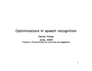
blake blake blake blake blake blake

b b b b b b

l l l l l l

ey ey ey ey ey ey

k k k k k k

11 10 3 2 2 1

p b l t p p

l ey l ey ey k ax l ax l l ey

k k ey k ey k

Figure 1: Realizations of the word “blake.” The second column is the expected dictionary pronunciation; the last column is the observed realization.

it has been spoken, along with counts of these events. This is illustrated in Figure 1 for the word “blake.” This indicates that “blake,” with dictionary pronunciation “b l ey k,” has been seen eleven times as “p l ey k,” ten times in expected form, twice as “t ax l ey k,” and so forth. Note that since we base the index on actual realizations, unexpected pronunciation variability (and system error) is modeled: in this case, we will learn that “p l ey k” is a pretty good indicator of “blake.” From the set of realizations, we create a single vector representation for each word. The terms (e.g. bi-phone pairs) for each realization are extracted, weighted with the realization count, and accumulated. Then, the term-frequencies are computed for the word, along with the IDF weights of the terms. Finally, a TF-IDF vector is created for each word. The reverse index is straightforwardly created, with one modification for efficiency: a word w will not occur in the reverse index (short-list) for term t if fewer that k% (typically 10%) of the realizations of the word contain t. In the example above, “blake” would not be placed on the short-list of “t ax,” since they have been seen together just twice out of 29 occurrences of “blake”. Without this type of restriction, the reverse index becomes unmanageably large. 2.4. Extensions We have found that two modifications to the log-TF-IDF score have a beneficial effect on accuracy. 2.4.1. Length Cost The presence of terms with very low IDF values will have little effect on the cosine distance; they are essentially invisible. However, they do represent the presence of acoustic units in a hypothesized word, and we have found it beneficial to model this. If we denote the number of units within a segment by n, one way of doing this is to explicitly tabulate P (n|wi ) for each word wi . This probability can then be weighted and combined with the log-TF-IDF score. We have found a simpler and equally effective method is to simply assume that the lengths are distributed according to a gaussian distribution. If li is the average number of units in a realization of word wi , and ns the number actually observed in a hypothesized segment s, the length score is then defined as α(li − ns )2 with some constant α. 2.4.2. Exact Match Score A linear combination of log-TF-IDF score and the length score can be used as a surrogate for the acoustic score to produce good word lattices. The one-best accuracy is improved, however, by making the following modification. Let AC(s, i) be the acoustic score associated with postulating word wi as the

label for segment s. Let seq(s) ∈ pron(i) denote the event that the unit sequence present in the segment is an exact match to a dictionary pronunciation of wi . We now define:  0 if seq(s) ∈ pron(wi ) AC(s, i) = log-TF-IDF(s, i) − α(li − ns )2 otherwise In other words, an exact match to a dictionary pronunciation is allowed zero cost. If a word is always realized in its dictionary form (and has just one pronunciation), this will happen anyway; but typically it is seen in a variety of realizations, so the TFIDF vector will be “diffuse” and the log-IF-IDF score would not otherwise be zero.

3. Recognizer Structure In this section we describe how the TF-IDF acoustic model is used in the recognizer. Note that the TF-IDF scores are inherently segmental, and unlike standard GMM-based scores, they cannot be accumulated frame-by-frame or unit-by-unit. Thus the recognition process is segmental rather than framesynchronous. Recognition is done as an offline process, and proceeds in two steps. First, for every possible segment within the utterance, a shortlist of words is created. Theoretically, if there are k units detected in the utterance, there are O(k2 ) possible segments. In practice, words are almost never more than 15 phonemes long, and so by restricting the segment length, the computational complexity becomes linear. After the set of candidate segment/word combinations is created, a dynamic programming search is performed to find the best scoring word sequence, including the application of an n-gram language model. These steps are now described in more detail. 3.1. Finding Word Candidates Let cand(i, j) be the set of words which are deemed to be reasonable matches to the segment starting with the unit at position i and ending at position j, inclusive. Denote the expected length of word w by len(w). Denote the length of the segment by len(s) = j − i + 1. We compute cand(i, j) for all i and j as follows: 1. Create the term vector from the units present in the segment. 2. For each term t in the vector, add word w to cand(i, j) if w is on the inverse index for t, and |(len(w)−len(s)| < δ. For phoneme units, δ = 4 works well. 3. Let LM (w) be the log of the unigram language model probability of w. Assign a score to word w equal to AC(s, w) + βLM (s), i.e. a weighted combination of the unigram LM score with the TF-IDF based acoustic score. 4. Sort the word candidates on the assigned scores. 5. Keep the N-best words (e.g. 50) as candidate labels for the segment. 3.2. Finding the Best Word Sequence After the sets of candidate words for each possible segment are collected, a simple dynamic programming search is made; this applies a general n-gram language model, and finds the best word sequence. It is essentially identical to that presented in [8], with just two features defined for each segment: the logTF-IDF score and the language model score.

Index Biphone Triphone Multi-phone

Oracle 31.4% 31.1 36.1

Outdegree 2.2 2.3 2.4

Runtime 0.09 xRT 0.11 0.0005

1-best 36.7% 36.4 38.1

Table 1: Decoding results with TF-IDF AM and trigram LM. Sentence error rate (SER) is reported for the oracle and 1-best lattice paths. The average outdegree for lattice nodes is provided as a measure of lattice complexity.

FM/DM Beam 10/5 50/50 50/100 50/150 Transducer HMM Decoder

Oracle 31.1 % 27.5 26.2 25.6 29.4 25.4

Outdegree 2.3 19 44 79 2.1 1.5

Runtime 0.09 xRT 0.20 0.27 0.35 0.008 1

1-best 36.4% 36.4 36.4 36.4 36.4 35.2

Table 2: Sentence error rate with TF-IDF AM, trigram LM and empirical pronunciations as a function of beams, and comparison with Transduction and HMM baseline.

4. Experimental Results 4.1. Voice Search Data Our first set of experimental results concerns mobile voice search data, collected from the Bing Mobile cell-phone client [13]. This is a mobile phone application with which users can request business information by voice. Typical queries are “Leo’s Bar & Grill” or “Mexican Restaurants.” When there is uncertainty in the speech recognition results, the n-best results are presented to the user to choose between or reject. To test the TF-IDF acoustic model, we used about 1200 hours of speech and the corresponding user selections to build a basic ML-trained speech recognition system with about 11k acoustic states and 260k gaussians. Multi-phone acoustic units were identified using the procedure of [15]. To build the TF-IDF index, we used two sources of data: • A phonetic dictionary • The actual acoustic realizations of a held-out set of 1200 hours of data. To get these realizations, we trained a multi-phone based trigram LM, and decoded using multi-phone units as “words.” Whereas the dictionary pronunciation of a word conveys our prior knowledge, the actual realizations will reflect pronunciation variability, as well as the error characteristics of the multiphone detection process. The dictionary pronunciations are simply added to the set of realizations (with count 1) prior to building the index. Following [5], we split the multi-phone detections back to phonemes, and then built phoneme based indexes. This results in a smaller number of basic indexing units, and has proven better than both using the multi-phone units directly and detecting phonemes directly. Our test set consists of 8777 utterances with hand-transcribed references. In Table 1, we show the effect of using different indexing units on sentence accuracy. A trigram word-level language model is used in these experiments. We see that a triphone based index produces slightly better accuracy, though with slightly larger lattices. Note that the biphone and triphone representations are actually formed by taking multi-phone output, break-

Method biphone, 10/20 triphone, 10/20 triphone, 30/90 triphone, 30/150 Transducer HMM Decoder

Oracle 9.1 8.8 7.3 6.8 9.8 3.7

Outdegree 6.5 7.5 35 66 1.1 2.2

Runtime 0.14 xRT 0.17 0.66 1.0 0.092 1

1-best 16.7% 16.3 16.3 16.3 14.4 9.7

Table 3: Wall Street Journal results. Lattice oracle and 1-best results are reported as word error rate (WER).

Method Transduction TF-IDF AM

Oracle WER 2.9% 1.9

1-best WER 3.2% 3.2

Table 4: Word error rates using the correct phonetic sequences. ing it down to the phoneme level, and then using phoneme n-grams. Using the multi-phone units directly is significantly worse, though because there are many fewer per utterance, and the index is smaller, the decoding time is very fast. In Table 2, we show the effect of adjusting the decoding beams, and compare results with phone-to-word transduction with an error model [9], and the HMM baseline. The FM (fastmatch) beam is the number of word candidates returned for each segment (c.f. Section 3.1). The DM (detailed-match) beam is the number of hypotheses propagated from any time step in the secondary dynamic programming search. The transducer produces n-best lists which we then converted into lattices; native lattice generation would likely produce somewhat better results. We see that with the TF-IDF approach, while 1-best accuracy plateaus even at tight beams, the oracle accuracy steadily increases. 4.2. Wall Street Journal Data The experimental results of the last section indicate that the TF-IDF acoustic model performs well with voice-search data. However, the average length of such utterances is just over two words, raising the question of how well the approach will work for longer utterances. To answer this question, we have applied the method to Wall Street Journal data. To make the acousticunit decodings, we trained a conventional HMM system on the WSJ SI-284 data, comprising about 72 hours of data taken from 284 speakers in both the WSJ0 and WSJ1 distributions (LDC93S6B,LDC94S13B). Results are reported for the open vocabulary 20k development set, and we used the distributed ARPA trigram language model. We have not yet applied MMI multi-phone unit decoding to the WSJ data, and instead have used pronlex syllable inventory (LDC97L20). After decoding at the syllable level, we broke the syllables down into phonemes to create the TF-IDF index. Both dictionary and realized pronunciations were used to make the index. Using this same acoustic model and language model in a conventional HMM decoding produces a 9.7% word error rate. Table 3 presents results on this task. We see that while the TF-IDF acoustic model does not produce 1-best results at the level of a HMM decoding, the lattice oracle error rate is reasonable, and the process is suitable for its intended purpose as a fast match for subsequent processing. To understand whether this is due to any inherent limitations in the modeling process, we performed an experiment with oracle input, in which the input pho-

netic sequence corresponded to that expected on the basis of the dictionary. The results are shown in Table 4; both transduction and TF-IDF decoding produce a 1-best 3.2% WER. Further, the TF-IDF approach achieves an oracle error rate of 1.9%, which is the best possible since the out-of-vocabulary rate is also 1.9%. Thus, it appears that the limiting factor is the quality of the input, rather than a fundamental limit on possible model performance.

5. Conclusion In this paper, we have extended the TF-IDF modeling of [5] for use in continuous speech recognition. The model is used to produce a segment level acoustic score which is combined with a standard n-gram language model. The search for the best word sequence is done with a segment-level dynamic programming algorithm. We find that this procedure produces good results in a voice-search task, and lattices with a reasonable oracle error rate on the Wall Street Journal task. The development of this method brings us one step closer to being able to do speech recognition based on the detection of sub-word audio attributes.

6. References [1] G. Salton, A. Wong, and C. S. Yang, “A Vector Space Model for Automatic Indexing,” Communications of the ACM, vol. 18, no. 11, 1975. [2] C. Manning, P. Raghavan, and H. Schutze, Introduction to Information Retrieval, Cambridge University Press, 2008. [3] M. Wechsler and P. Schauble, “Speech retrieval based on automatic indexing,” in Proc. MIRO, 1995. [4] E. Chang, F. Seide, H. Meng, Z. Chen, Y. Shi, and Y. Li, “A System for Spoken Query Information Retrieval on Mobile Devices,” IEEE Transactions on Audio, Speech, and Language Processing, 2002. [5] X. Xiao, J. Droppo, and A. Acero, “Information Retrieval Methods for Automatic Speech Recognition,” in ICASSP, 2010. [6] M. Bacchiani, J. Hirschberg, A. Rosenberg, S. Whittaker, D. Hindle, P. Isenhour, M. Jones, L. Stark, and G. Zamchick, “SCANMail: audio navigation in the voicemail domain,” in Proc. HLT, 2001. [7] H. Li, Bin Ma, and Chin-Hui Lee, “A Vector Space Modeling Approach to Spoken Language Identification,” IEEE Transactions on Audio, Speech, and Language Processing, vol. 15, no. 1, 2007. [8] G. Zweig and P. Nguyen, “A Segmental CRF Approach to Large Vocabulary Continuous Speech Recognition,” in Proc. ASRU, 2009. [9] G. Zweig and J. Nedel, “Empirical Properties of Multilingual Phone-to-Word Transduction,” in ICASSP, 2008. [10] C-H. Lee, “From Knowledge-Ignorant to Knowledge-Rich Modeling: A New Speech Research Paradigm for Next Generation Automatic Speech Recognition,” in ICSLP, 2004. [11] G. Zweig and P. Nguyen, “Download available at http://research.microsoft.com/en-us/projects/scarf/default.aspx,” 2010. [12] G. Zweig and P. Nguyen, “SCARF: A Segmental Conditional Random Field Speech Recognition Toolkit,” in Submitted to Interspeech, 2010. [13] A. Acero, N. Bernstein, R. Chambers, Y.C. Ju, X. Li, J. Odell, P. Nguyen, O. Scholz, and G. Zweig, “Live Search for Mobile: Web Services by Voice on the Cellphone,” in Proc. of ICASSP, 2007. [14] D. Paul and J. Baker, “The Design of the Wall Street Journal Based CSR Corpus,” in Proc. HLT, 1992. [15] G. Zweig and P. Nguyen, “Maximum Mutual Information Multiphone Units in Direct Modeling,” in Proc. Interspeech, 2009.