The RAND Corporation
Dynamic R&D Competition with Learning Author(s): David A. Malueg and Shunichi O. Tsutsui Reviewed work(s): Source: The RAND Journal of Economics, Vol. 28, No. 4 (Winter, 1997), pp. 751-772 Published by: Blackwell Publishing on behalf of The RAND Corporation Stable URL: http://www.jstor.org/stable/2555785 . Accessed: 21/11/2011 07:12 Your use of the JSTOR archive indicates your acceptance of the Terms & Conditions of Use, available at . http://www.jstor.org/page/info/about/policies/terms.jsp JSTOR is a not-for-profit service that helps scholars, researchers, and students discover, use, and build upon a wide range of content in a trusted digital archive. We use information technology and tools to increase productivity and facilitate new forms of scholarship. For more information about JSTOR, please contact
[email protected].
Blackwell Publishing and The RAND Corporation are collaborating with JSTOR to digitize, preserve and extend access to The RAND Journal of Economics.
http://www.jstor.org
RAND Journal of Economics Vol. 28, No. 4, Winter 1997 pp. 751-772
Dynamic R&D competition with learning David A. Malueg* and Shunichi 0. Tsutsui**
To account for the possibility that firms are unsure about the ease of innovation, we formulate a differential game of R&D competition with an unknown hazard rate. We show, as time passes without success, firms become more pessimistic about eventual innovation, reducing their R&D investment and possibly exiting the race. An increase in the number of competing firms tends to increase firms' R&D intensities, for given beliefs, but because beliefs evolve at different rates depending on the number of firms in the race, time paths of R&D investment intensity are not unambiguously ordered with respect to the number of competing firms.
1. Introduction * Previous stochastic patent-race models featured a probability of innovation governed by an exponential distribution with known hazard rate parameter (see, for example, Loury, 1979; Lee and Wilde, 1980; Reinganum, 1981, 1982, 1983; Grossman and Shapiro, 1987; Dixit, 1988; Hung and Quyen, 1993; and Lin, forthcoming). The memoryless feature of the exponential distribution implied that even if a decade had passed without innovation, firms viewed themselves in the same position as when the patent race had begun. Consequently, even if fully dynamic research and development (R&D) strategies were allowed (as in Reinganum, 1981, 1982), constant strategies (assumed in Lee and Wilde, 1980) turned out to be optimal (Malueg and Tsutsui, 1995a). While constant R&D strategies provide a tractable environment for comparative statics analyses, such strategies seem unreasonable in an environment in which learning should be a central consideration. Indeed, one of the most important characteristics of R&D is its riskiness. Riskiness encompasses more than just the stochastic timing of innovation. As Jorde and Teece (1990, p. 76) wrote, "[innovation] involves uncertainty, risk taking, probing and reprobing, experimenting, and testing. It is an activity in which 'dry holes' and 'blind alleys' are the rule, not the exception." Thus, in many "high-risk" R&D projects, it seems likely firms are not sure whether they can succeed, even if an active R&D effort is maintained. The project may be impossible to complete, but no one knows this for * Tulane University; dmalueg @mailhost.tcs.tulane.edu. ** KPMG Peat Marwick; stsutsui@ kpmg.com.
While retaining responsibility for any remaining errors, the authors wish to thank two anonymous referees for their comments on an earlier version of this article. Copyright (C 1997, RAND
751
752
/
THE RAND JOURNAL OF ECONOMICS
sure ex ante. In such a case, a more accurate assessment of the project's difficulty develops while research is being done on the project. All of this suggests that firms have only imperfect knowledge about the distribution governing the timing of innovation in high-risk R&D projects. For example, in a survey of thirteen major chemical firms, Mansfield et al. (1971) found that only three of the firms gave more than 20% of their R&D projects a chance of technical success in the 75-100% range. One firm in the survey estimated that 80% of its projects had technical success probabilities in the 0-20% range. Regarding actual successes of R&D projects, Mansfield et al. studied 220 R&D projects at three laboratories (one chemical laboratory and two proprietary drug laboratories). They distinguished three probabilities: the probability of technical completion of a project, the probability of commercialization (given completion), and the probability of market success (given commercialization). Over the entire sample of projects, the probability of technical completion was .57 (that is, the laboratories were successful in meeting the technical objectives of 57% of the projects). As one would expect, the probability of success depended on the size of the hoped-for advance. Small advances had a 66% chance of success; medium advances, 42%; and large advances, 26%. Only 55% of those projects having technical success went on to be commercialized, and only 38% of those commercialized went on to be successful in the market. Thus, for the three laboratories in question, the probability of market success, given that the project is begun, turned out to be only 12% (- .57 X .55 X .38). Choi (1991) first analyzed a patent race with an uncertain hazard rate. In his model, the probability distribution governing each firm's innovation was exponential, with the unknown hazard rate taking on one of two values. As time passed, firms updated their beliefs about the hazard rate. Choi allowed, however, only a very simplistic R&D strategy: a firm in the patent race engaged in R&D activity at a fixed (exogenous) intensity; a firm's only decision was whether to be in the race. In such a fluid environment, though, a dynamic approach like Reinganum's (1981, 1982) is most appropriate. Concluding his essentially static analysis of R&D that combined the approaches of Loury (1979) and Lee and Wilde (1980), Dixit (1988, p. 326) wrote, "Perhaps the most important aspect ignored here is the possibility of partial progress (state variables) in the R&D race. That has so far proved intractable at any reasonably general level, but remains an important problem for future research." The current article attempts such an analysis. We extend Choi's model to accommodate variable R&D investment intensities. To do this, we use Reinganum's (1981, 1982) differential-game model of a patent race, with the additional assumption that firms are uncertain about the hazard rate governing the innovation process. In keeping with Choi, we specify the unknown hazard rate in such a way that the R&D project is either solvable or unsolvable (in Appendix B we provide an alternative formulation in which the hazard rate is distributed according to a gamma distribution). We solve our differential game of R&D competition by applying the method of dynamic programming. To our knowledge, this article is the first to characterize the solution to a differential game in which there is learning about the environment. In this way, it makes a technical contribution to the theory of differential games that may be applicable beyond the literature on dynamic R&D. Regarding the economics of R&D, we provide the following results. First, as firms exert R&D effort, the failure to innovate leads them to become more pessimistic about the difficulty of innovation-they attach greater likelihood to the project's being more difficult to complete. In Choi's model, too, failure to innovate led firms to become more pessimistic about eventual success. In contrast to Choi's model, though, in our model the rate at which firms become more pessimistic is itself endogenous because beliefs depend on the endogenously determined R&D intensities. Second, the value of being in the patent race declines as firms become more pessimistic about innovation. Third, we provide
MALUEG AND TSUTSUI
/
753
examples showing that as the number of firms in the patent race increases, each firm's intensity of R&D increases-holding beliefs fixed. But because the greater intensity of R&D causes firms to become pessimistic quicker, the time paths of R&D intensity can actually cross. That is, late in the race, if no innovation has yet occurred, the race with more firms may have firms engaging in R&D at lower intensities than if there had been fewer firms. In the continuous-uncertainty model of Appendix B, we show that even with continuous revision of R&D intensities, market structure has the same effects on expected R&D investments as shown by Loury (1979): an increase in the number of firms in the race reduces each firm's expected R&D investments but increases the aggregate expected R&D expenditures.
2. The model * We consider an infinite-horizon model with n identical firms competing for an the same for all firms. innovation. The value of the patent on the first innovation is 1AT, Firms' common discount rate is r. Consequently, a patent awarded at date t has a time0 value of ireft. Losers in the race receive no rewards. Following Reinganum (1981, 1982), we assume firms' chances of winning the race depend on the state of accumulated knowledge. We assume the state of knowledge across firms at any date is common knowledge; in particular, firms' R&D activities are commonly observed. (Alternatively, one could assume that R&D intensities are only privately observed. In that case, the open-loop solution would be appropriate for the R&D game.)' Firm i acquires knowledge according to the differential equation z!'(t) = u(t, z(t)), where zi(t) denotes firm i's accumulated knowledge at date t and z(t) = (zl(t), . . ., zj(t)) denotes the state of knowledge of all firms at date t. The function uf(t, z) denotes the investment strategy of firm i at date t, given the state of knowledge is z. We assume the initial state of knowledge
is zero: zi(O) = 0, i = 1, . . ., n. In pursuing R&D strategy ui, firm i incurs
an instantaneous flow cost of c(ui), where c(ui) = f + uI2 for ui > 0, and c(O) = 0. We interpret f as a "flow fixed cost." Costs are also discounted at the rate r. Following Reinganum (1981, 1982), we assume the amount of knowledge a firm needs to produce an innovation is exponentially distributed with mean 1/4t, where 11' 0 is an unknown parameter (the same ,u applies to all firms); thus, given ,u, the probability of an innovation by a firm with accumulated knowledge equal to z is 1 - edz. Smaller values of ,u represent greater difficulty of innovation. Our central assumption is that firms are uncertain about the value of the hazard rate. The evidence cited above from Mansfield is consistent not only with a project's being impossible, but also with its simply being more difficult than initially expected. In either case, firms may cease working on a project after they have gathered more information about its difficulty. For simplicity we suppose that ,u takes on one of only two values: the project is either unsolvable (denoted U) and ,u = 0, or the project is solvable (denoted S), in which case ,u = A > 0. (Alternatively, one might model the project as being "easy" or "difficult" without being impossible. The analysis then follows that presented in the text, with the extra complication of considering whether R&D is profitable when the project is known to be "difficult.")2 Firms have common initial beliefs about ,u, with Po denoting the prior probability that the project is unsolvable, and 1 - po denoting the probability that the project is solvable. Conditional on ,u, the levels of knowledge needed by each firm in order to innovate are independent and identically distributed. IWe prefer here to follow the previous literature by assuming that R&D intensities are observable. This assumption has some support, too, considering the types of reports that a publicly held firm must file with the SEC (e.g., Form 10-K), some of which disclose R&D expenditures. 2
The hazard rate might also be modelled
as a continuous
in which prior beliefs are described by a gamma distribution.
random variable. Appendix
B treats the case
754
/
THE RAND JOURNAL OF ECONOMICS
The conditional probabilities of an innovation for a firm with stock of knowledge equal to z are given by F(z IU) = 0 and F(z IS) = 1 e-Az. Therefore, letting ti denote the random time at which firm i innovates (i.e., completes the project), we see the conditional probabilities that firm i innovates before time t are given by -
Pr(ti '
t| U) = F(zi(t)I U) = 0
Pr(ti < tIS)
and
F(zi(t)IS)
=
= 1 - eAzi(t).
With the above probability structure, we obtain Pr(t, > t, .
,t,, > t I U)=1
and Pr(t1 > t,
...,
tn > tIS) = Pr(t1 > tIS)Pr(t2 > t1S) ...
Pr(t,, > t1S) =
e-40,
from which the unconditional probability that no firm has innovated by date t is found to be Pr(t1 > t,
(1)
t,, > t) = po + (1 - po)e-Azk(t)
. . .,
Because firms only imperfectly know the hazard rate, the news that no firm has completed the project by time t provides additional evidence that the project is unsolvable. Given no firm has succeeded by time t, the probability the project is unsolvable, p(t), is calculated by Bayes' rule as
p(t) -Pr(U|I
t, > t, ...,
t,, >)
p
+ (1
-
)
po)eA
(2)
Differentiation of (2) shows, for given investment strategies, that beliefs evolve according to the differential equation dpt) dpt)
=
AE
(t,
(t)))p (t) ( I
(3)
p(t)).
Because dp(t)ldt > 0 as long as there is some uncertainty about ,u and at least one firm is investing in R&D (E uf(t, z(t)) > 0), firms become increasingly pessimistic about the project's solvability as the race continues without innovation. The probability density function for firm i's date of innovation, conditional on the project's being solvable, is dF(zi(t) IS)Idt = Auf(t, z(t))eAz(t). Therefore, given conditional independence of the firms' probabilities of success, the probability density for the event that firm i is the first to innovate and does so at time t is calculated as follows: Pr(ti = t; tj > t, j # i)
=
poPr(ti = t; tj > t, j # iI U) + (1 - po)Pr(ti = t; tj>t,
= (1 - p0)Au#(t,z(t))e-Azkt Po(1 - p(t)) A (t
(t
j
i S)
MALUEGAND TSUTSUI /
755
For a given vector of investment strategies, u = (uI, . . ., u,), the present value of firm i's instantaneous expected payoff at time t is, given positive R&D effort, = t; tj > t, j # i)'nr - Pr(t1 > t, . . . , tl > t)c(ui))
e-rt(Pr(ti
(p0(
kp0(t)
=
-
p(t))
AU
A(
PO -
____
f +
Integrating over time, we find the associated expected discounted payoff to firm i is t
Po((l
- p(t))7TAu((t,
Z(t)))2)
where Tj is the date at which firm i drops out of the patent race if no innovation has yet occurred.
3. The equilibrium value function and R&D strategies *
We seek the feedback equilibrium to the patent race described above. This equi-
librium is given by a vector of investment
strategies u = (u1, .. ., u,), such that at
every date, firm i finds it optimal to continue its strategy ui, given the current date and the state of the system and the rivals' strategies, i = 1, . .. , n. In light of (4), we view
p(t) (rather than z(t)) as the state variable of the system and, therefore, write ui as a function of p, not z. To analyze these "continuation games" in deriving the feedback equilibrium, we introduce the value function Vi(t, p), which specifies the maximum value to firm i at date t, given time-t beliefs parameter p, taking as given the investment strategies of the rivals. Optimality of firm i's investment strategy requires
Vi(t,p) = max IT e -rs Tislj(-)
such that dp(s) ds
Ps ((1
-
p(s))
p(s))rAuj(s,
-
f-
(U(S' P(S)))
p (S)
t
(
) ds
2(5)
u,(s p(s)))p(s)(1
and p(t) = p.
- p(s))
A solution ui to (5) must satisfy the following system of Hamilton-Jacobi-Bellman (HJB) equations (see Lee and Markus (1986) for a standard derivation of the HJB equation):' -Vi(s,
p) = maxe
-rs((1
-
p)7TAUi
-
f
-
+
+jV
(6)
for all "initial conditions" (s, p), where -; is a fixed investment strategy of rival j, j 0 i, i, j = 1, . . ., n. In (6), Vtiand VPidenote the partial derivatives of Vi with respect to its first and second arguments. The derivation of the patent-race equilibrium now reduces to solving
the HJB equations.
Because
Vi(t, p) = p0Ipe-rtVi(0,
p), where
p = p(t), in looking for a solution to the HJB equation we naturally look for a solution I Here a firm's strategy is an R&D intensity function and a belief threshold at which it exits the race. Because the HJB equations essentially work "backward" from the terminal condition, with current actions affecting future actions through their effects on future beliefs, these equations incorporate a firm's recognition
of its ability to affect rivals' future actions.
756
/
THE RAND JOURNAL
OF ECONOMICS
among the following class of functions: Vi(t, p) = (poIp)e-rIv(p). From (1) and (2), we see that the prior probability that there is no innovation by date t is equal to Pr(tj > t, . .. ,tn, > t) = polp(t).
Therefore, v(p) is understood as the conditional value function: in equilibrium, for belief parameter p, v(p) represents the expected value to firm i from continuing optimally, given no innovation has yet occurred. For the class of value functions being considered, the maximizer of the right-hand side of (6) is u* =
(
+ pv'
p)(-i
- v).
(7)
Equation (7) implies a firm's optimal R&D intensity depends only on current beliefs, not time. Therefore, we henceforth express u* as a function of current beliefs, p, only and not the date t. For this reason, the point at which a firm optimally exits the race will be given in terms of terminal beliefs rather than a terminal date. Substituting (7) for all firms into (6), the HJB equation reduces to the following functional equation that must be satisfied by the equilibrium conditional value function: 2rv = A2(1
-
p)2(ir + pv' - v)(ir
(2n -
-
I)v + (2n -
I)pv')
-
To understand the equilibrium solution of the HJB equation, we solve (8) for g(p,
V=
(8)
2f. V :4
V)
-A(1 - p)(nir
-
(2n - I)v) + V(n (2n -
-
-
l)2A2r2(1
I)Ap(I
p)2 + 2(2n - 1)(f + rv)
- p) (9)
The curve COin Figure 1 depicts the locus where v' = 0. The equation for this curve is
v
=
go(P) + nirA2(1
-[r -
V'(n-
* [(2n-
)2
-
1)2ir2A4(1 1)A2(l
(10) -
p)4
+ 2nrirA2(1
-
p)2 +
r2
+ 2f(2n
-
1)A2(1 - p)2]
-p)2].
sloping because ago(p)lap < 0, for 0 < p < 1. Also, the the two points (0, vo(n, f)) and (1, - fir), where
The curve CO is downward curve
CO connects
vo(n,
f)
r + nA2ir =
\/r2
+ 2nrA2ir + (n - 1)2A4ir2 + 2(2n - 1)A2f (2 )2(11)
Using CO, we can draw the family of solution curves that satisfy (9). Below CO, v' is negative; above CO, v' is positive. Therefore, below CO all solution curves are decreasing, while above CO they are increasing. Figure 1 plots some of these solution 4Equation (8) is quadratic in v', so there are two solutions for v'. In (8) we have taken the solution as the larger root because the other solution is economically nonsensical-for example, it implies negative investments in R&D.
MALUEG
AND TSUTSUI
I
757
FIGURE 1
000 O
"
-~~~~~~~~~~~~~P
curves. The differential equation (9) has two singular points, one at (0, vo(n,f)) and one at (1, -f fr). The curve COintersects the horizontal axis (v = 0) at j- = 1 - \/(7j(An-T). We assume the fixed flow cost f is such that j-> 0.5 Because the point (0, vo(n, f)) in Figure 1 is a node, infinitely many solution paths for the differential equation (8) emanate from this point. We see from (9) that v' approaches -oo as p approaches zero from above; also, (10) implies curve COhas bounded slope zero at p = 0. Therefore, the solution curves to the differential equation (8) start from (0, vo(n, f)) and, at least initially, fall below CO.Some of the curves continue to decrease and cross the horizontal axis; others decrease, cross the curve CO, and thereafter increase. Which of these is the economically meaningful solution? First, the solution curve must not cross the horizontal axis, because a firm can always assure itself at least a zero payoff simply by not engaging in R&D; consequently, v should never be negative. Second, the solution curve cannot cross the curve COin Figure 1, for any curve that does will approach infinity as p increases toward 1-but this is absurd because v(p) cannot exceed -,T.Therefore, at least where v(p) is strictly positive, the equilibrium solution curve begins at (0, vo(n,f)) and is decreasing, lying between the horizontal axis and COin Figure 1. We summarize these results in the following proposition. Proposition 1. The equilibrium conditional value function v(p) is strictly positive and 1 - \ fI(Anr-), with v(O) = vo(n,J) and limPt- v(p) = 0. strictly decreasing for 0
K A2ir2/2.The case of f 2 A2ir2/2 is
trivialbecause no firm engages in R&D.
758
/
THE RAND JOURNAL OF ECONOMICS
exit belief level is independent of the number of firms in the race.6 To see that j5 is independent of r, just recall that at the dropout date, a firm is indifferent between dropping out of the race and continuing for just an "instant" longer. Whether such continuation is profitable does not depend on the interest rate if the "instant" considered is sufficiently short. We next establish properties of the equilibrium conditional value function v(p). Proposition 2. For 0 ? p < j: (i) av(p)lan < 0, (ii) av(p)lar < 0, (iii) av(p)lIeT> and (iv) av(p)1dA > 0.
0,
Proof See Appendix A. The properties reported in Proposition 2 are intuitive. An increase in n means the race is more competitive, reducing the value of being in the race. An increase in r, however, reduces the present value of any positive flow of expected benefits; so, too, the equilibrium conditional value of continuing the race falls with r. Increases in the value of the innovation, r, or the speed with which it arrives, A, raise the value of being in the race. Using (9) in (7), we can now express the equilibrium R&D intensities as U
(n
-
l)Akr(l
-
p) 4- V'(n
-
1)2 A2I2(l (2n- 1)
-
p)2
? 2(2n
-
l)(f ? rv)
(12)
for p < P. Because the equilibrium conditional value function, v(p), is nonincreasing in pa the following proposition follows immediately from (12). Proposition 3. The feedback equilibrium R&D strategy, us, is a strictly decreasing function of p for all p < P. For all p > j, u* = 0. Therefore, equilibrium R&D intensities
decrease over time and limptj u*(p)
=
I.
Proposition 3 implies that if f = 0, then the race continues until an innovation occurs, with the race possibly lasting forever. But if f > 0, then duration of the race can be bounded. This occurs either because a firm innovates or because beliefs reach P- in finite time, the latter outcome arising because u* ' \/27 while the race continues (i.e., R&D intensities are bounded away from zero).7 Recall that polp(t) is the probability that no firms succeed by time t. Taking the limit of this fraction as t -- oo, we have the following result. Corollary 1. If po < )5, then in the feedback equilibrium the ex ante probability of no innovation ever occurring is po/jl = (Air/(Ar f))po. Corollary 1 shows that the probability of an innovation does not depend on market structure, but its timing will. When f > 0, the probability of innovation exceeds the prior probability that the project is impossible. This reflects the finding that when f > 0, there are two reasons for failure to innovate: first, the project may be impossible; second, even if the project is not impossible, firms may become sufficiently pessimistic about the prospects for success that they choose to drop out of the race. 6 Firms' simultaneous exit is related to Proposition 5, below. Without any fixed cost of entering the patent race, being engaged in the race is of value to no firms (no entry), or it is valuable to everyone (infinite entry). If firms varied in their flow fixed costs, we would expect differing dropout dates (and multiple equilibria!). 7 This bound on af and (2) imply that if po < T, the race ends by date
(An<'7)-
log[((l
-
p0)/p0)((Ai -T
MALUEG AND TSUTSUI
/
759
In general, we are unable to provide comprehensive comparative static results regarding the equilibrium R&D strategies.8 However, Proposition 2 and (12) imply the following: Proposition 4. For 0 ' p < j,
au*(p)/aig>
0 and au*(p)/aA > 0.
Note that the comparative statics reported in Proposition 4 are for a given level of beliefs p. It is also natural to ask how the time path of R&D evolves. Using particular examples, in Section 5 we provide a more detailed analysis of equilibrium R&D strategies and their time paths.
4. Endogenous
market structure
* We have so far assumed that the market structure (namely, the number of firms in the race) is given. Without restrictions on entry, however, it seems reasonable to expect an additional firm to enter the patent race whenever the entrant'sexpected profit is positive. It is easily seen from Proposition 1 and equation (11) that if the conditional value function is positive for some number of firms n, then it is positive (at the same initial beliefs) for all numbers of firms. Moreover, from (11) we see that lim,. vo(n,f) = 0. Consequently, we have the following proposition. Proposition 5. If po < -, then each firm's expected profit in the R&D race is strictly positive and approaches zero as the number of firms in the race approaches infinity. Loury (1979) obtained a result similar to our Proposition 5. It is interesting to note that a flow fixed cost does not generally impose an upper bound on the number of firms that can make nonnegative expected profit by participating in the race. This is because even with positive flow fixed cost, as the number of firms increases, the race ends almost immediately, as some firm innovates or the updated beliefs quickly reach j5. Hence, the impact of the flow fixed cost becomes negligible. So with unrestricted entry, atomistic competition is likely to appear with or without a flow fixed cost. The number of firms in the race can be bounded, however, if firms must incur an upfront cost. Let K denote the upfront cost a firm pays to enter the patent race. This might include unrecoverable costs associated with building a research laboratory. Then the maximum number of firms, n*(K), that enter the patent race is the largest integer n for which v(po)l,, > K. Because the conditional value function v(p) is decreasing in both n and p, for p < p, we have the following proposition. Proposition 6. The free-entry equilibrium number of firms, n*(K), in the patent race is a decreasing function of the upfront cost of entry, K, and a decreasing function of the initial beliefs, po. Though we envision the entry phase occurring before firms engage in R&D, our results would not change if entry were allowed during the race. Because firms become more pessimistic as the race progresses without success, any firm unwilling to pay the upfront fee K initially will be unwilling to enter the race at a later date.
5. Examples * A = 1, r = 10, and r > 0. In this subsection we use numerical simulations to investigate properties of the equilibrium. From Propositions 2 and 5, the roles of A and 8 The difficulty arises because for r > 0, the conditional value function, v, enters the equilibrium strategy given by (12), and v is itself found as the solution to the differential equation (9). The properties of the differential equation (9) have not been sufficient for us to establish properties of u, for all p E--), [0,
beyond those in Proposition 5.
760
ir
/
THE RAND JOURNAL
OF ECONOMICS
are clear. Therefore, in this subsection we do not vary these parameters and simply
specify A = 1 and rr= 10.
We know from Proposition 2 that an increase in competitiveness of the R&D race, as represented by an increase in n, will decrease the value of being in the race (that is, v(p) falls as n increases). Next, Figure 2 depicts the equilibrium R&D strategy u*(p) for n = 2, 3, and 4. This figure shows that for given beliefs p, as n increases, firms increase their R&D intensities. This extends the result found by Lee and Wilde (1980) for the case of p = 0. Notice that the three belief paths of R&D terminate at the same point, (j-, \/f) (see Propositions 1 and 3). Because the presence of more firms in the race leads each firm to invest more at every belief level, an increase in the number of firms in the market causes knowledge to accumulate quicker, causing beliefs to change more quickly. This is depicted in Figure 3, which shows that the time path of beliefs, p(t), is shifted up by an increase in the number of competitors. Recall that the ex ante probability that some firm innovates by date t is 1 - (po/p(t)). Therefore, the effect illustrated in Figure 3 implies that an increase in the number of competitors in the race leads to an earlier date of first innovation in the sense of first-order stochastic dominance. Finally, consider the effect of n on the time path of equilibrium R&D intensities. The time path of an individual firm's equilibrium R&D intensity is given by u*(p(t)). As reflected in Figure 2, an increase in n leads to greater R&D, for each given level of beliefs. But Figure 3 shows that this, in turn, makes firms become pessimistic more quickly if the race proceeds without success. So for two races differing only by the number of firms, the one with more firms begins with each firm exhibiting a greater R&D intensity; but as those firms become more pessimistic than the firms in the less crowded race (at the same point in time), the firms in the more competitive race may exhibit lower R&D intensity than do the firms in the less crowded race. Such a crossing of equilibrium R&D time paths is illustrated in Figure 4. Two other parameters worth investigating are the interest rate, r, and the flow fixed cost, f. In simulations, we have found that an increase in r leads firms to increase their R&D intensities as a function of p. This leads to a quicker accumulation of knowledge and the crossing of time paths of R&D as r increases. The role of the flow fixed cost is, perhaps, more interesting. FIGURE 2 u~(p)
6
-
L 0
~~~I .2
I .4
I .6
I .8
Parameterspecification: n= 2, 3, 4; f= 1; r= 1/100; A= 1; ir= 10
p
MALUEG AND TSUTSUI
/
761
FIGURE 3 p .8 -=
.61 -<
.2
0
.4
.8
.6
Parameterspecification: n= 2, 3, 4; f= 1; r= 1/100 A = 1; r= 10; po = 1/100
An increase in f raises the cost of remaining in the race. Therefore, a lesser degree of pessimism is sufficient to induce firms to exit the race (that is, j- is decreasing in f). In this sense, an increase in f leads to less R&D (by Corollary 1, an increase in f lowers the equilibrium probability of an innovation ever occurring). However, an increase in f leads firms to increase their R&D intensities while actively in the race: an earlier innovation date now has the added benefit that the higher flow fixed cost can be avoided sooner. This is shown in Figure 5, which depicts the equilibrium R&D intensities as functions of beliefs; Figure 6 depicts the time path of R&D intensities as f varies, given initial beliefs po = .01, which also shows an increase in R&D intensities. Thus, an increase in f has opposing effects: it causes firms to compete more intensely, but they exit the race sooner if no innovation occurs. The first of these effects tends
FIGURE 4 u*(t) n= 4 8 -
n= n= 2 6
4
2
0
I .2
I .4
I .6
.8
Parameterspecification: n = 2, 3, 4; f= 1; r= 1/100; A = 1; r= 10; p0 = 1/100
762
/
THE RAND JOURNAL OF ECONOMICS
FIGURE 5 u*(p)
4 _-
5
.2
0
.4
p
.6
f= 1 Parameterspecification: n= 2; f= 1, 2, 3; r= 1/100; A= 1; r= 10
toward earlier innovation dates, but the latter tends toward lower probability of eventual success. Consequently, the effect of f on the date of first innovation cannot be described by first-order stochastic dominance. 0 r = f = 0. The findings above are based on numerical simulations. In this subsection we assume r = f = 0, and, to ensure that an equilibrium exists, we assume n ? 2. The simulations suggest that the findings below are robust. Although it is likely that firms' discount rates are positive, if we assume no discounting, then we can explicitly derive properties of the equilibrium. (Moreover, in Appendix B we derive closed-form solutions for the equilibrium strategies and expected R&D costs.) Positive discount rates keep firms from delaying costly actions "too" much. FIGURE 6 u*(t) 7-
6-
5
4
3f= 3 f=2 0
.2
.4
.6
.8
f= 1 Parameterspecification: n= 2; f= 1, 2, 3; r= 1/100; A= 1; ir= 10; Po = 1/100
MALUEG AND TSUTSUI
/
763
The presence of rival firms fulfills this role because a firm delaying R&D too much risks losing the race to a rival. As a result, our comparative statics findings when there are at least two firms in the race might reasonably be expected to resemble those we would find if the equilibrium could be explicitly calculated for positive discount rates.9 For r = f = 0, the differential equation (9) simply reduces to v (p)
-
-(2n
-
l)v(p)
IT
(2n- 1)p which, with boundary condition v(1) = 0, is integrated to
( _
v(p)=
2n
)
(13)
I
As reported in Proposition 2, (13) shows that an increase in the number of firms in the patent race reduces the value of being in the race. The equilibrium R&D strategies follow immediately from (12) and (13): U*(P) = 2(n
1)AIr(I
-p)
(14)
2n-1I Equation (14) reveals that, holding beliefs constant, an increase in the competitiveness of the patent race leads each firm to increase its level of R&D. This extends Lee and Wilde's result beyond the case of po = 0. Substituting (14) into (3), we see that beliefs evolve as follows:
dp(t)
-
2n (n- 1)
such that p(O) = Po.
-rA2p(t)( I-p(t))2
(15)
Equation (15) can be integrated, yielding the solution for p in implicit form:
I 1- p(t)
P + log(
p(t))
I1- P(tj
2n (n =
2nn
I~ +rAi( + 1tA
+
2n-II1P
l
+ log
Po\ _ kI -Po/
(16)
Because the left-hand side of (16) is increasing in p(t), we have the following result, which describes how variations in the model's parameters affect the accumulation of knowledge in the patent race. Proposition 7. If r = f = 0 and n" > n', then in the feedback equilibrium, p(t)j,,=,, > P(t)L,,=,, for all t > 0, provided no innovation has yet occurred. Also, increases in A, Ir, or po increase p(t). Because the ex ante probability that some firm innovates by date t is I - (polp(t)), Proposition 7 and (16) imply the following:
Proposition 8. If r = f = 0, an increase in n, A, or
Ir leads to an earlier date of innovation in the sense of first-order stochastic dominance. An increase in po leads to a later date of innovation in the sense of first-order stochastic dominance. 9 The reason to assume n : 2 is that a monopolist could always reduce its expected cost of R&D by pursuing a slightly less aggressive R&D strategy, without affecting the overall chance of eventual success. Because r = 0, a firm is indifferent about the timing of innovation. However, the presence of rivals in the patent race (n ' 2) is sufficient to keep firms from investing too slowly in R&D.
764
/
THE RAND JOURNAL
OF ECONOMICS
FIGURE 7 u*(t) 8
6
4
2
0
.2
.4
.6
.8
1
Parameterspecification: n= 2, 3, 4; f= r= 0; A= 1; r= 10; pO= 1/100
We have seen that an increase in the number of firms in the patent race increases R&D intensities, given p. But because beliefs then evolve more rapidly with more firms in the race, it is possible that the time paths of equilibrium R&D intensities would cross as the number of firms in the race increases. This is indeed the case, as shown in Figure 7. An increase in the number of firms increases R&D intensities near the beginning of the race,'0 but if no innovation occurs, firms quickly become more pessimistic about success than if there had been fewer firms and so, later in the race, R&D intensities are lower with more firms in the race. Because we are unable to get a closed-form solution for the equilibrium R&D strategies, we are unable to obtain expressions for equilibrium expected R&D costs. Such a calculation is useful because one interpretation of the seeming difference in Loury's (1979) and Lee and Wilde's (1980) results is that Loury's conclusions were about the effects of competitiveness, n, on expected R&D costs per firm, whereas Lee and Wilde's referred to the effects on each firm's R&D intensity while the race continued. It is quite possible that an increase in n will increase each firm's R&D intensity while lowering each firm's expected R&D costs because the race with greater intensities ends sooner, thus reconciling Loury's results with Lee and Wilde's. This relationship is indeed found for the model described in Appendix B, where the prior beliefs about At are described by a gamma distribution. There we show that for given beliefs, an increase in n will increase each firm's R&D intensity while decreasing each firm's expected total R&D costs. Also extending Loury, we show in Appendix B that an increase in n increases expected R&D expenditures for the market as a whole, even though each firm's expected R&D expenditures fall.
6. Conclusion * This article has considered a Bayesian approach to dynamic R&D competition. To execute this analysis we adopted Reinganum's (1981, 1982) dynamic formulation, with the addition that firms only imperfectly know the stochastic process governing innovation. This allows for nontrivial learning-as time passes without innovation, '0 Analytically, this follows from (14).
MALUEG
AND TSUTSUI
/
765
firms revise their beliefs about how much additional R&D will be needed for an innovation. In previous analyses of R&D competition with known hazard rate, firms' beliefs do not change. For this reason, the static approach of Lee and Wilde (1980) coincided with Reinganum's (1981, 1982) dynamic analysis (Malueg and Tsutsui, 1995a). An advantage of our approach is that it yields realistic dynamics. Failure to innovate is taken as evidence that the project is more difficult than initially believed. This leads firms to gradually decrease their R&D intensities over time. Similarly, the value of being in the patent race falls over time as firms become more pessimistic about the prospects for success. Finally, we also found, at least for the special case of no discounting, that the effects of market structure on innovation are consistent with those found in earlier static models: increasing the number of firms in the race makes earlier times of innovation more likely, and it reduces each firm's expected R&D costs but increases expected R&D costs in the aggregate. Appendix A *
1 and 2 follow.
Proofs of Propositions
Proof of Proposition 1. We prove that the proposed behavior constitutes denote the solution to the following differential equation:
p(t)= dt
nAu*(p)p(l
- p),
firms' equilibrium
such that p(O)
strategy. Let p(t)
po.
that is, T is the time at which beliefs reach p, given that all firms are using the Let T be such that p(T) =; proposed equilibrium strategies uO. Using the HJB equation, we have
r(U
1T p
fpoe-rs
=
f|; f
[(1
-
p(S))ITAu*(p(s))
[-vi-
ViA(2
[-Vt-
VPj dt
uj*(p(s)))
*(p(s)))21 2
-
p(s)(1
-p
(s))]
]|ds
ds
ds
p (s))) ds
= I-(-Vi(s, dt
= Vi(O,p(O)) - Vi(T, PMT) =v( p) =
-
er-(p
-Po
V(Po),
0. This where the first equality follows from the HJB equation (6) and the last follows because v(T) proves the validity of the conditional value function. Next we show that the firm cannot improve its payoff by dropping out at a belief threshold less than or greater than T3. Suppose first that firm i chooses to drop out at j, where fi < T. Let xi(p) be firm i's R&D investment strategy for 0 ' p ' 0. Let 6(t) denote the solution to the differential equation d1 (t) dt
Let T be such that O(t) =.
A(xi(,b) + (n
Now suppose
l)u*( ,,
n, f))p(1
--p3),
such that p(0) = po.
all firms but i play u*, and player i plays xi until dropping out
when beliefs reach ip. The associated expected payoff to firm i is given as
766
I
THE RAND JOURNAL
OF ECONOMICS
espS) '
(1- -3(s))1TAx2((s))-f-
[-V,- Vi A(xi(I
fo
f[vt JT
(s)) +
| d
______
ds
uj*( (s)))I(s)( l -p(s))
E
Pd3
_V
dV
(s)|
Vi(s, j (s)))ds
-(-
=
(xi(I5(S)))21d
X ' S)
Tper____,T Jo
dt
= Vi(0, (0)) - Vi(T, fi(T)) v~p 1p
-
= v (po)
e -riT
v(po),
where the first inequality follows from the HJB equation and the last follows because v(p) 2 0. This proves that dropping out before beliefs reach T is not an optimal response by firm i to its rivals following strategy uO. Next, suppose firm i chooses to drop out at j3, where fl > Pj. Let xi(p) be firm i's R&D investment strategy for 0 ' p ' f. Let fi(t) denote the solution to the differential equation
dg(t) = A(xi(fi) + (n -
dt
s.t. p3(O) = po.
(1 - p3),
l)u*(fi))P
Let T be the date such that p(T) = j3. (Note that u* = 0 after date T. So after date T, only firm i is active.) Let T be such that P(T) = P. By the same argument as in the previous case, the HJB equation implies that
p-rs tpoe
Therefore,
(1
I
f
-
- f(s))1TAx(P(s))
-
ds '
(Xi(p(S)))]
)
v(p
the payoff to firm i is given as
Jo
JPoe p-rs
+
[ 1 (s))1T7Axi(1(s)) - p -(xir~j~~))t
()(
fopoe-s
-fi(s))rrTAx((fi(s))
[(1
T
(P?)ft
(1
-
pear
1(S))ITAxi(P3(s))
-
)[(1
f
-
-
f
|
+
ds
2]ds
-(xi(13(S)))2l
-
e(-) fPs
P(s)1-
ds
_ ( i(I(
-2(s))Ax;(P(s))-f
(x1i
Po-r VP
( ' PS) 2
-
____
fpoe?( +
-
) ] ds
(x(1(S)))21 p(s))1TAxs(p(s))
d
f
-
d
Now observe that the final integral in the previous expression is just the expected payoff to a single firm pursuing strategy xi, having beliefs P, given there are no other firms in the race. But recall that T is independent of the number of firms in the race. Therefore, this last integral must be nonpositive, from which it follows that T
-
-rt Jo
implying that dropping following strategy uO.
e
XS)
(1
-
fi(s))ITAxi(fi(s))
out at the beliefs Q.E.D.
-(xi.(fi(S)))2]
-
(;
)
ds _ v(po),
greater than Ti is not an optimal response
Lemma 1. For 0 < p < T: (i) dg/dn 2 0 (with equality only at p = p), (ii) dg/dr v = 0), (iii) dg/dlrr < 0, and (iv) dg/dA < 0.
?
by firm i to its rivals 0 (with equality only if
MALUEG AND TSUTSUI Proof.
Define A = (n - 1)2 A2(1 (i) From (9), we see that
-
p)2
7T2
(n - 1)A27T2(1-
dg an
+ 2(2n -
I
767
+ rv). Note that for p < T, v(p) > 0.
1)(f
TVA - 2(2n - 1)(f + rv) + A(1 (2n 1)2Ap(l -p)A
p)2
The numerator of the above fraction is positive
if v < h(p)(v
(negative)
where
f
A27T2(1 - p)2
_
> h(p)),
2r
r
Now consider the graph of v = h(p) in the (p, v) plane. We now show that this graph is located above the curve C0 for 0 ' p < p. Observe that because v = h(p) implies 2(f + rv) = A2 7T2(1 - p)2, it follows that
A|1(P) = (n - 1)2A27r2(1 -
(2n
+
p)2
-
1)A272(1
-
(nAT(I
p)2
-
p))2.
Consequently,
g
V
-
-() =-A(
p)(nIT
-
-
v > 0,
(2n l)v) + nArT(1 - p) I)Ap(1 - p)
-
(2n
P
which implies that the graph of v = h(p) is situated strictly above C0 for 0 ' p
Oc
>
0 for
p < p. (ii) Here we find dg/dr = v/(Ap(l (iii) Here we find
dg d)IT
- p)VA)
1I (2n -
which is readily seen to be strictly negative (n - 1)4A27T2(1
p)2
- n2A
0, with equality only when v
?
(n - 1)2A7T(1-p)\
|
I )p
0.
kV/
because
-A2IT2(1
-
p)2(n -
1)2(2n -
1) - 2n2(2n - 1)(f + rv) < 0.
(iv) Finally, we see that dg dA
-
1)(f + rv)
1)p(l
-p)A2V/
-2(2n (2n -
<
Q.E.D.
0 for all values of n : 2 (recall that p- is independent Proof of Proposition 2. (i) First observe that v(p) of n). Furthermore, v'(p-) = g(p- 0) = 0 (see (9)). Therefore, the second-order Taylor series approximation
of v(p) near T is v(p)
v(p) + v'(F)(p - F) +
v"2
(p - F ()2
P(P 2
F)2
While the general expression for v"(p) is rather involved, from (9) it is relatively easy to show that at p-, - p)). Therefore, the second-order Taylor series approximation becomes v"(p-) = ,/(np((l
(P)
which is obviously
decreasing
2np(l
in n. Therefore,
IT - p)(P
-pF 2.
if n" > n', then for some E
v(p)l,,=,,.
<
>
0,
v(pAl,",=
for all p e (p - P, p). Also, it is readily verified that vj(n", f) < vo(n', f). Now suppose, contrary to the proposition, that the graphs of v 4,,. and v|,,= do intersect at some point p e (0, p-). Then it is the case that v~p|,,,,= vp)|,=, =v^> 0 and, from Lemma 1, dg( p, v^)/dn> 0, which together imply v'(p)|,,=,, > v'(p)|,,,, .
768
/
THE RAND JOURNAL
OF ECONOMICS
Because v' < 0, this last inequality says that if graphs of v|,,=,, and v|,,=,, do intersect at some point jb E (0, f), then the graph of v|,,=,, is strictly less steep than the graph of v|,,=,, at (pi, v). But this implies the graphs cross at most once in the interval (0, P) so that v(p)|,,=,, > v(p)|,,=,, for all p E (i, P), which contradicts the - E, P). Therefore, it must be the case finding above that for some E > 0, v(p)|,,=,, < v(p)|,,=,, for all p E that v(p)|,,=,, < v(p)|,,=,, for all p E [0, ). (ii) To analyze the impact of the interest rate r on v(p), we consider the third-order Taylor series expansion for v around P: v"(f)
-
v(p)
v(p)
+ v'(p) (p - p) +
-
IT
2np(1
2
-
(p p)3 -
6 term in the above approximation.
dr E >
Also, we can show that
~~~~IT
_ _ __
if r" > r', then for some
6
_ __(p
- p)
Notice that r does not enter the second-order
Therefore,
v"1(fl)
(p-p)
n2Ap2(l -p)2N/2 0,
V(p)_r=r
<
v(P)lr=r
for all p such that j - E < p < j. Also, it is readily verified that vo(n, fAr=, < vo(n, )jr=r` Because dg/dr > 0 for all p < p (Lemma 1 (ii)), it follows as in part (i) above that the graphs of vj,.-r and vlr=r do not intersect at any point strictly between zero and p. > P= (iii) It is readily checked that PI=, and vo(n, f),r=, > vo(n, f)l,.,, for 7T" > 7T'. Because dg/dlrT< 0 for all p < PI,, (Lemma l(iii)), it follows as in part (i) above that the graphs of v r` and vj| do not intersect at any point strictly between 0 and P (iv) This is proven in the same way as part (iii). Q.E.D.
Appendix B U This Appendix recasts the dynamic R&D game with firms' initial beliefs characterized by a gamma distribution. The gamma prior is very flexible, including the exponential and chi-squared distributions as special cases. Also, for appropriate specification of parameters, the gamma approximates a normal distribution. The model presented is identical to that in Section 2 except for the specification of prior beliefs and, for simplicity, the assumption of no flow fixed cost (i.e., f = 0). We assume that the firms' common prior beliefs about A are represented by a gamma distribution with parameters ao > 0 and b > 0; specifically, the for all A > 0, where F(-) denotes the density representing prior beliefs is f(Ajao, b) = (abAb- e -A)/F(b),
gamma function. Because lower values of A represent greater difficulty of innovation, an increase in ao represents more pessimistic beliefs in that greater weight (in the sense of first-order stochastic dominance) is put on lower values of A. For this distribution the mean and variance are E[A Iao, b] = b/ao and var[A Iao, b] = b/ao . We assume, given A, that firms' innovation processes are stochastically independent and R&D intensities are commonly observed. With this probability structure, the following probabilities are readily verified: Pr(t1 > t, ...,t,
> t IA)
e-A Zk(t)
and Pr(tj = t; tj > t, j =$ i IA) = Auj(t, z(t))e-A
Zk(t),
where the second equation is understood as the density function for the event that firm i wins the patent race at time t, given the hazard rate is A. Letting a(t) = ao + I zk(t), we find
(aa(tJ
Pr(t, > t,..,
t, > t)
e-Akzk()f(A
ao, b) dA =
f(AIa(t),
b) dA =
(Bl) a(t))b
MALUEG AND TSUTSUI
Pr(tj = t; tj > t, j =$ i)
769
Iao, b) dA =abu(t,
z(t)) (a (t))b+lI
Au(t, z(t))e-A;zk(1)f(A
=
I
Finally, posterior beliefs, given no innovation has occurred by time t, are calculated as > t, . ; nt > t IA)Pr(A)_ t,, > t) =Pr(t, > t, . ~~~~~Pr(t, t,,> t)
Pr(A|Itj > t,
Pr(Ajt1>t
(a(t))bAb-le-Aa(t)
F7(b)
thus, posterior beliefs at time t are described by a gamma distribution with parameters a(t) and b. For a given vector of investment strategies, u = (ul. ..), u the present value of firm i's instantaneous expected payoff at time t is e-rt(Pr(tj = t; tj > t, j =$ i)I7 - Pr(t1 > t,
= e -rt( abT
t, > t) 2
at)
Integrating over time, we find that the associated expected discounted payoff to firm i is taobbui(t, z(t)),7T_ab(U,(t,
( J0
(a (t))b+
\
I
Z(t)))2
d(2
2(a (t))b
In light of (B2), we view a(t) (rather than z(t)) as the state variable of the system and, therefore, write ui as a function of a, not z. The value function Vi(t, a) specifies the maximum value to firm i at date t, given time-t beliefs parameter a, taking as given the investment strategies of the rivals. Optimality of firm i's investment strategy requires
1(
U&()
(_
da (s) /d(aO da
such that
(s, a (s)))2
abbui(s, a(s))I7T _ab(U,
V~(t,a) = max
ds
(a(s))b+1 +
da)
14k(s))\
)
/
ds
d (B3)
2(a(s))b
=
and
Uk(S, a(s))
a(t)
=
a.
A solution ui to (B3) must satisfy the following HJB equation:
-Vi(s, a)
Fabbui.1T e uiL\ab+1
max
=
-rsI
-+
1
a~buj\ + b 2aJ
iaVa
+
g
j
} Ja(4
(B4)
for all "initial conditions" (s, a), where Tijis a fixed investment strategy of rival j, j =$ i, i = 1,. n. In solving the HJB equation, we look among the following class of functions: Vi(t, a) = (a b/ab)e-rnv(a). The function v(a) is understood as the conditional value function: in equilibrium, for belief parameter a, v(a) represents the present expected value to firm i from continuing optimally, given no innovation has yet occurred. For the class of value functions being considered, the maximizer in (B4) is
*=
-(bIT + av' - bv). a
(B5)
Equation (B5) implies that a firm's optimal R&D intensity depends only on current beliefs, not time. Therefore, we express u* as a function of current beliefs only. Substituting (B5) for all firms into (B4), the HJB equation reduces to the following functional equation that must be satisfied by the equilibrium conditional value function:
rv
=
-(bIT
2a2
+ av' - bv)(bIT + (2n - 1)(av'
-
bv)).
(B6)
To understand the equilibrium solution of the HJB equation, we solve (B6) for V: -b(nIT
-
(2n
-
1)v) + '\/(n - 1)2b2ir2+ 2(2n (2n - 1)a
-
1)ra2v .(7
770
THE RAND JOURNAL OF ECONOMICS
/
Solutions to (B6) and (B7) can be analyzed as in the case of the two-point proofs can be found in Malueg and Tsutsui (1995b).
prior. Here we report our results;
Proposition B]. For r > 0, the equilibrium conditional value function v(a) is strictly positive decreasing, with v(0) = I7/(2n - 1) and limao v(a) = 0. Using (B7) in (B5), we can express the equilibrium R&D intensities as follows:
U* =
Because
v(a) is a nonincreasing
Proposition equilibrium
(n
i1
(nab
+
. 2(2n -
(n-i2b
function of a, the next proposition
follows
and strictly
8)
1)rv)
(B8)
from (B8) and Proposition
B2. The feedback equilibrium R&D strategy, u*, is a strictly decreasing R&D intensities decrease over time and limtx u*(a(t)) = 0.
B1.
function of a. Therefore,
Because the conditional value function v(a) is nonnegative, it follows that a firm's expected R&D expenditures are finite. Nevertheless, Proposition B3 shows that the expected time to innovation may be infinite. Proposition B3. Suppose ao > 0, b > 0, and let t* denote the random time at which the patent race ends in the feedback equilibrium. If b ' 1, then the expected date of first innovation is infinite; that is, E[t*] = oo. In general, we cannot solve the differential equation (B7) and (B8). However, for the special case of r = 0, we can derive explicit formulas for v and u*, giving an exact characterization of the feedback equilibrium to the patent race. Therefore, for the remainder of this Appendix, we assume r = 0 and n : 2. Though the case of r = 0 may seem unrealistic, it is valuable in that it provides an analytical reinforcement of the patterns found numerically for the case of r > 0 in Section 5. In this case, the differential equation for v(a) can be solved explicitly: v(a) = IT/(2n - 1). The corresponding R&D strategy is
u*(a)
= 2(n-
1)bl7 1)a
(2n-
(B9)
This solution has intuitive properties: increases in i7 and reductions in n raise the expected payoff. In agreement with Lee and Wilde (1980) and Reinganum (1981, 1982), for given belief parameter a, increases in n raise firms' equilibrium R&D intensities. Moreover, as time passes without an innovation, firms become increasingly pessimistic about the ease of success, and they correspondingly continuously reduce their R&D intensities. From (B3) and (B9) we see the equilibrium path of beliefs is described by the differential equation = 2n(n
d (a(t))(a(t))
dt with the boundary
condition
a(O)
=
a0. The solution
a(t)
Using (B1) and (B10) we can calculate
-
-n(a))=(2n
to this differential
a2 + 0 4n(n-
=
2n
the expected
1)b)t)
1)a (t) equation is
(B10)
1)blTt -1
time of innovation
for the case of no discounting.
Proposition B4. Suppose r = 0, ao > 0, and b > 0. Let t* denote the random time at which the patent race ends in the feedback equilibrium. If b ' 2, then the expected date of first innovation is infinite; that is, E[t*] = oo. If b > 2, then the expected date of first innovation is finite; in particular,
E[t*]
-
(2n - I)ao n(n - 1)(b - 2)blrT
For the case of b > 2, Proposition B4 shows that the expected date of innovation has intuitive properties. In particular, increasing the number of firms or increasing the value of the prize reduces the expected date of innovation. For the case of b ' 2, however, the expected time to innovation is too coarse a measure to discern the effect of market structure. Nevertheless, the effect of market structure is clear in terms of firstorder stochastic dominance. Proposition B5. Suppose r = 0, ao > 0, and b > 0. Let t* denote the random time at which the patent race ends in the feedback equilibrium. Then increasing the number of firms in the patent race leads to an earlier
date of innovation, t*, in the sense of first-order stochastic dominance.
MALUEG AND TSUTSUI
/
771
To evaluate how market structure affects expected R&D costs, we next find the exact equilibrium strategies. Substituting (B10) into (B9), we find the time path of R&D intensity is
R&D
us
-)blT
_2(n
2n - 1 2(n-
1
1
a2
+ 4n(n
0
E[A ao, b]
1)IT
1
2n-
)bT
2n -1(B)
-|1 +
n(n 2n
-
-)7Tvar[A
1
ao, b]t
From (B11) it follows that a greater patent value, 7T, or more favorable initial beliefs (smaller ao) lead to higher R&D intensities. Equation (B 1 1) also reveals the role of prior uncertainty. If expected project difficulty, E[A Iao, b], is held constant while the variance of prior beliefs is reduced, the time path of R&D intensity increases, converging, as prior variance goes to zero, to the intensity found in the certain-hazard-rate case (see (14) for the case of po = 0 and A = b/ao). Finally, as prior variance is reduced, the time path of R&D intensity becomes less responsive to time, reflecting that greater time is needed to change the less diffuse beliefs. The time path of R&D expenditures expressed in (B 1 1) exhibits the same crossing behavior with respect to market structure as found in the two-point prior distribution analyzed above. Suppose m > n 2 2. Then for the race with m firms, individual R&D intensities are initially greater, but there is some (finite) date To such that for all t > To, if there has been no innovation yet, individual R&D intensities are lower with m firms than with n firms in the race. Even though the patent race can be expected to last infinitely long, firms' expected R&D costs are finite. This finiteness occurs because as time passes without innovation, firms quickly reduce their R&D intensities toward zero. Let ETC(n) denote an individual firm's expected total R&D expenditures in the feedback equilibrium with n firms.
Proposition B6. Suppose r = 0, a0 > 0, b
>
0, and n 2 2. Then ETC(n) = (n - 1)IT/[n(2n - 1)].
The following corollary to Proposition B6 shows that the role of market structure for equilibrium expected R&D expenditures is as described by Loury (1979): an increase in n lowers expected R&D expenditures at the individual firm level, but increases expected R&D expenditures in the aggregate.
Corollary BL. Suppose r = 0, a0 > 0, b
>
0, and n 2 2. Then d(ETC(n))/dn < 0 and d(n
X
ETC(n))/dn > 0.
References CHOI, J.P "Dynamic R&D Competition Under 'Hazard Rate' Uncertainty." RAND Journal of Economics, Vol. 22 (1991), pp. 596-610. and Policy." RAND Journal of Economics, Vol. 19 DIXIT, A.K. "A General Model of R&D Competition (1988), pp. 317-326. GROSSMAN, G.M. AND SHAPIRO, C. "Dynamic R&D Competition." Economic Journal, Vol. 97 (1987), pp. 372-387. HUNG, N.M. AND QUYEN, N.V. "On R&D Timing Under Uncertainty: The Case of Exhaustible Resource Substitution." Journal of Economic Dynamics and Control, Vol. 17 (1993), pp. 971-991. JORDE, T.M. AND TEECE, D.J. "Innovation and Cooperation: Implications for Competition and Antitrust." Journal of Economic Perspectives, Vol. 4 (1990), pp. 75-96. LEE, E.B. AND MARKUS, L. Foundations of Optimal Control Theory. Malabar, Fla.: Robert E. Krieger Publishing Co., 1986. LEE, T. AND WILDE, L.L. "Market Structure and Innovation: A Reformulation." Quarterly Journal of Economics, Vol. 94 (1980), pp. 429-436. LIN, P "Product Market Competition and R&D Rivalry." Economics Letters, forthcoming. LOURY, G.C. "Market Structure and Innovation." Quarterly Journal of Economics, Vol. 93 (1979), pp. 395410. MALUEG, D. AND TSUTSUI, S. "Market Structure and Innovation: Constant R&D Intensities Are Optimal." Mimeo, Tulane University, 1995a. . "A Bayesian Analysis of R&D Competition When the Difficulty of Innovation Is AND Unknown." Mimeo, Tulane University, 1995b. MANSFIELD,E., RAPOPORT,J., SCHNEE, J., WAGNER, S., AND HAMBURGER,M. Research and Innovation in the Modern Corporation. New York: W. W. Norton and Company, 1971. Journal of Economic Theory, Vol. 25 (1981), pp. 21-41. REINGANUM, J.E "Dynamic Games of Innovation."
772
/
THE RAND JOURNAL OF ECONOMICS
. "A Dynamic Game of R and D: Patent Protection and Competitive Behavior." Econometrica, Vol. 50 (1982), pp. 671-688. . "Uncertain Innovation and the Persistence of Monopoly." American Economic Review, Vol. 73 (1983), pp. 741-748.