Exits from Recessions: The U.S. Experience 1920-2007†
Michael D. Bordo, Rutgers University and NBER John Landon-Lane, Rutgers University
December 2009
Paper prepared for the Conference Volume, “No Way Out: Government Response to the Financial Crisis” edited by Vincent Reinhart. American Enterprise Institute
†
For helpful comments and suggestions we thank: Joesph Haubrich, Owen Humpage, and David Wheelock. For valuable research assistance we thank Emel Yildirim.
1
Exits from Recessions: The U.S. Experience 1920-2007
Abstract
In this paper we provide some evidence on the issue of when a central bank should shift from expansionary to contractionary monetary policy after a recession has ended—the exit strategy. We examine the relationship between the timing of changes in several instruments of monetary policy and the timing of changes of selected real macro aggregates and price level (inflation) variables across U.S. business cycles from 19202007. We find, based on historical narratives, descriptive evidence and econometric analysis, that in the 1920s and the 1950s the Fed would generally tighten when the price level turned up. By contrast, since 1960 the Fed has generally tightened when unemployment peaked and this tightening often occurred after inflation began to rise. The Fed is often too late to prevent inflation.
2
Exits from Recessions: the US experience 1920-2007
1. Introduction
The recession of 2007-2009 is now over and the U.S. economy is recovering. Real GDP grew at slightly less than 3% in the third quarter of 2009. Monetary policy has been very expansionary since the fall of 2008 (as has fiscal policy). The Federal Reserve reduced the funds rate from 5.25% in August 2007 to close to zero by January 2009. The question now arises over how to return its policy to one consistent with long-run growth and low inflation—the exit strategy. To do this involves switching from expansionary to a neutral monetary policy, reducing the Fed’s balance sheet and for fiscal policy, reducing the large fiscal deficits and increases in the national debt.
The key question is when should this happen. At present there are two views to this subject. One view argues that because of the financial crisis, the credit crunch and the large overhang of nonperforming loans and toxic assets that the recovery will be slow and that the need to tighten will not occur for quite some time. This view is backed up by cross country evidence which demonstrates that recessions accompanied by financial turmoil tend to be deeper and longer (Claessens et al 2008, Reinhart and Rogoff 2009). The alternative view is that the recovery will be V shaped as was the case in most of the severe recessions in the U.S. in the twentieth century (Mussa 2009).
3
The risks facing monetary policy with respect to the exit strategy are twofold: tightening too soon and creating a double dip recession and tightening too late leading to a run up of inflation. There are a number of famous historical examples of each type of error. Tightening too soon after the Great Contraction led to the recession of 1937-38. Tightening too late in the recessions of the 1960s and 1970s contributed to the Great Inflation.
In this paper we provide some evidence for this issue by examining the historical record of U.S. business cycles from 1920 to the last full cycle which peaked in December 2007. Our approach is to first provide a brief historical narrative on each of the cycles. ( Section 2) . We then present descriptive evidence in section 3 on the timing of policy change from ease to tightness and on the changes of macro aggregates around the lower NBER turning point of each cycle. We divide the sample in two: cycles before World War II from 1920 to 1938; and cycles from 1948 to the present.
To supplement the descriptive analysis we then run some simple regressions in section 4 of the timing of policy changes relative to the trough of the real variables (real GNP, industrial production, the output gap, and unemployment) and price variables (inflation and the price level pre 1960). In section 6 we use the coefficients of the effects of the timing of the indicator in the postwar period to predict the possible exits from the current recession. Section 7 concludes.
4
We can discern some basic patterns across the historical experience. In general in the post WWII period the Fed tends to tighten when inflation (the price level) is rising and postpones tightening when the output gap and unemployment have yet to turn. However the decision to wait until unemployment (the output gap) turns, dominates the decision to tighten when inflation rises. The timing of tightening differed somewhat before and after World War II. In the pre WWII era the Fed would generally tighten when the price level turned up. This could cause it to tighten too soon. In the post WWII era the Fed, by focusing on unemployment tended to err on the side of tightening too late, i.e. after inflation resurged.
We also find that there are a few cycles when the Fed got the timing just right and followed a countercyclical policy. 1 These were in the 1920s and 1950s as earlier discussed by Friedman and Schwartz (1963) and Meltzer (2003, 2010). In most cycles Fed actions were procyclical.
We further note a significant difference between the cycles before 1965 when the Fed adhered to some form of gold standard convertibility rule and the Fed attached highest priority to price stability (Bordo and Eichengreen 2009) and the cycles since when the gold standard became a less important consideration and then did not matter at all. In the late 1960s and 1970s, the Fed generally waited until unemployment and the output gap declined before tightening and placed little emphasis on the pace of inflation. Since the Volcker shock in the early 1980s, the Fed has placed more emphasis on reducing
1
Friedman (1953) was the first to analyze the difficulty of achieving the pace and timing for successful countercyclical policy.
5
inflation than before in determining its exit strategy. A memorable episode in which the Fed tightened when unemployment was high and rising was in 1981 when Volcker was determined to break the back of inflation.
In the last two cycles, in the early 1990s and early 2000s the Fed, concerned with persistent unemployment (“a jobless recovery”), waited too long.
In the first case,
significant tightening occurred close to three years after the trough following “the inflation scare of 1994”. In the second case, the Fed, concerned with the risk of deflation, waited four years after the trough and accordingly may have ignited the housing price boom which burst in 2006 leading to the current recession. The recent episode with unemployment at over 10 per cent and low inflation may be similar to the two preceding cycles.
2. Historical Narrative: 1920-38
2.1. Peak January 1920, Trough July 1921. The recession of 1920-21 was one of the three worst recessions of the twentieth century. Friedman and Schwartz (1963) viewed it as the Fed’s first policy failure. They indict the Fed for waiting too long to raise rates to stem the inflationary boom that followed World War I and then for waiting too long to reverse the ensuing recession. The Fed waited until November 1919 to begin tightening because of pressure by the Treasury on the Fed to keep the prices of its wartime bond issues high. During the recession that followed, real GNP fell by 15%, industrial
6
production fell by 23%, the GNP deflator fell by 20% and the unemployment rate increased by 8%.
The cause of the recession was the Fed’s decision (triggered by a decline in its gold reserves), to implement a very rapid deflation, to roll back the run up in prices that had occurred since the U.S. entered World War I. The Fed raised the discount rate from 43/4% in January 1920 to 7% in June and kept it at that level until May 1921. The highly persistent rise in nominal interest rates in the face of a shift in expectations from inflation to deflation represented a much tighter policy stance than agents anticipated (Bordo, Erceg , Levin and Michaels 2007). In the face of mounting political pressure the Fed reversed course four months after the recession ended. IP recovered in August and by March 1922 had increased 20% above the previous year.
2.2 Peak May 1923, Trough July 1924. The recession of 1923-24 was relatively brief and by pre World War II standards mild, real GNP fell by 4%. The recession followed a tightening of monetary policy beginning in May 1922 which reflected concern that the rapid recovery from the previous recession was becoming inflationary. In contrast to the previous recession the Fed began reversing course soon after the recession became apparent in December 1923 with open market operations and then cuts in the discount rate in May 1924 (Meltzer 2003). Friedman and Schwartz gave the Fed high marks for conducting a successful countercyclical policy.
7
2.3. Peak October 1926, Trough November 1927. Similar to the recession of 1923-24, the Fed began tightening, reflecting fears of inflation, in January 1925 with open market sales and then a rise in the discount rate in February. As in the preceding recession, the Fed reversed course and began open market purchases in May 1927, halfway through the mild recession (Meltzer 2003).
2.4. Peak August 1929, Trough March 1933. The Great Contraction of 1929-33 during which prices, real GNP and the money stock (M2) declined by about a third, was the worst recession in U.S. history. Since Friedman and Schwartz (1963), it is widely attributed to policy failures at the Federal Reserve. Beginning in 1927 the Federal Reserve Board became increasingly concerned over stock market speculation and the growing boom on Wall Street. Based on the real bills doctrine many officials believed that stock market speculation was inflationary. The Fed began monetary restraint with open market sales in February 1928 and continued this policy through 1929 with a rise in the discount rate from 5% to 6% in August 1929.
The tightening while insufficient to halt the stock market boom was sufficient to induce a downturn beginning in August 1929. The Stock Market Crash in October 1929 exacerbated the downturn but did not cause the depression. The failure of the Fed to follow its mandate from the Federal Reserve Act of 1913 to act as a lender of last resort and to allay a series of four banking panics beginning in October 1930, led to the serious downturn that followed. A major hike in the discount rate in October 1931 to protect the dollar after sterling exited from the gold standard added fuel to the fire. Despite short
8
lived expansionary open market purchases in the spring of 1932 which if continued could have ended the recession (Friedman and Schwartz) the recovery in March 1933 was not precipitated by Fed policy.
Recovery began in March 1933 with Roosevelt’s banking holiday, ending the fourth banking panic. The nation’s banks were closed for a week during which an army of bank inspectors separated the insolvent banks from the rest. Insolvent banks were closed ending the uncertainty driving the panic. This action was quickly followed by FDR taking the U.S. off the gold standard in April, Treasury gold (and Silver) purchases designed to raise gold prices and prices in general, and formal devaluation of the dollar by close to 60% in January 1934. These policies produced a big reflationary impulse from gold inflows which were unsterilized passing directly into the money supply. They also helped convert deflationary expectations into inflationary ones (Eggertsson 2008).
The recovery of 1933 to 1941 was largely driven by gold inflows (initially reflecting Treasury policies and the devaluation, later reflecting capital flight from Europe as war loomed. Expansionary fiscal policy played only a minor role in the recovery of the 1930s (Romer 1992). Recovery was impeded somewhat by New Deal cartelization policies like the NIRA which in an attempt to raise wages and prices artificially reduced labor supply and aggregate supply (Cole and Ohanian 2004). Over the period 1933-37 output increased by 33%.
9
2.5 Peak May 1937, Trough June 1938. The 1937-38 recession, which cut short the rapid recovery from the Great Contraction of 1929-33, was the third worst recession in the twentieth century: real GNP declined by 10% and unemployment which had declined considerably after 1933 increased to 20%. The recession was primarily a consequence of a serious policy mistake by the Federal Reserve. Mounting concern by the Fed over the inflationary consequences of the build up in excess reserves in member banks (held as a precaution against a repeat of the banking panics of the early 1930s), led the Board to double reserve requirements in three steps between August 1936 and May 1937. Fed officials were concerned that these reserves would lead to an explosion of lending and would foster a reoccurrence of the asset price speculation of the 1920s. They also believed that reducing excess reserves would encourage member banks to borrow at the discount window. The Burgess—Riefler doctrine which prevailed at the time argued that the Fed could exert monetary control by using open market operations to affect member bank borrowing and hence to alter bank lending (Meltzer 2003).
The consequence of doubling reserve requirements in three steps from August 1936 to April 1937 was that banks sold off their earning assets and cut their lending to restore their desired cushion of precautionary reserves. The Fed’s contractionary policy action was complemented by the Treasury’s decision in late 1936 to sterilize gold inflows in order to reduce excess reserves. These policy actions led to a spike in short-term interest rates and a severe decline in money supply.
10
The recession ended after FDR in April 1938 pressured the Fed to roll back reserve requirements, the Treasury stopped sterilizing gold inflows and desterilized all the remaining gold sterilized since December 1936 and the Administration began pursuing expansionary fiscal policy. The recovery from 1938 to 1942 was spectacular; output grew by 49% fueled by gold inflows from Europe and a major defense build up.
Historical Narrative: 1948-2007
2.6 Peak November 1948, Trough October 1949. After the war, inflation increased to 15% per year by 1948. Tightening by both the Treasury and the Fed began in October 1947. A mild recession ensued beginning in November 1948. Real GNP fell by less than 2 %, IP by 9% and CPI prices fell by 2%. Fed policy was slow to change during the recession because the Fed viewed low nominal interest rates (T bills) at close to 1% as evidence of ease and didn’t realize that in the face of recession real rates were elevated. The Board reduced reserve requirements by 2% in May 1949. According to Meltzer (2003, chapter 7), 1948-1949 was similar to 1920-21 in that deflation by both encouraging gold inflows and increasing the real value of the monetary base helped to reinflate the economy.
2.7 Peak July 1953, Trough May 1954. After the Federal Reserve Treasury Accord of March 1951, the Fed was free again to use its policy rates to pursue its policy aims. One of the first occasions was at the end of the Korean War when both monetary and fiscal
11
policy tightened to prevent an increase in inflation. In January 1953 the Fed raised its discount rate and the real money base declined leading to a recession beginning in July. The real economy declined by 3.2%, IP by 9.4% and unemployment rose to 6.1%. However unlike earlier recessions the Fed eased policy in June 1953 to offset a spike in long-term Treasury bond rates. Ease continued with a decline in reserve requirements in July 1953 and a decline in the discount rate in February, April and May 1954 and declines in reserve requirements in June and July. By October 1954 with recovery well underway the Fed began to tighten in December in the face of incipient inflationary pressure. The Fed raised the discount rate in 7 steps from the end of 1954 to 1957. This was evident in a rise in ex post interest rates (Meltzer 2010 chapter 2, Friedman and Schwartz 1963 chapter 11).
2.8 Peak August 1957, Trough April 1958. Growing concern over the pace of recovery from the previous recession and a run up in inflation in 1955 led the Fed to begin tightening in April by raising the discount rate. Further increases followed in 1956. The ensuing recession was relatively mild with real GDP falling by 3% and unemployment rising to 7.5%. The Fed was slow to respond to the recession because of continuing concern over inflation (Meltzer 2010 chapter 2). It began easing in November 1957 by reducing the discount rate and reserve requirements and conducting open market purchases in March and April 1958. The recovery was vigorous and the Fed again worried about inflation began tightening (raising the discount rate) in August, four months after the trough. It was also concerned for the first time in the postwar period with gold outflows (Friedman and Schwartz 1963 page 618).
12
2.9 Peak April 1960, Trough February 1961. The Fed began tightening in the spring of 1959 in the face of rising inflation and gold outflows. By early 1960 the FOMC recognized that the economy had slowed and began to ease two months before the April business cycle peak, as it had done in 1953. The ensuing recession was mild and lasted 10 months. Real GNP fell by less than 1% and unemployment increased to 7%. Fed policy continued to be loose throughout the downturn, the discount rate was cut in March and august and reserve requirements were cut in August. The recession ended in February. After the trough the policy directive for ease was moderated in April (Meltzer 2010 chapter 3). The real federal funds rate began to rise one quarter after the trough and the growth of the real base slowed at the trough. Unemployment peaked in May.
2.10 Peak November 1969, Trough November 1970. The period from 1961 to 1964 exhibited very rapid growth with low inflation. Inflation began to rise in 1965. The Fed tightened in December 1965 against President Johnson’s wishes but not enough to stem rising inflation. Further tightening in the spring and summer of 1966 led to the “Credit Crunch” of 1966, a growth slowdown but not a recession (Bordo and Haubrich 2009). The Fed began tightening again in the summer of 1969 seen in a decline in real base growth and a rise in real interest rates leading to a mild recession which began in July 1969. Real GNP fell less than half a percent, unemployment increased to 5.9% and inflation only slowed moderately. Policy began to ease after January 1970 seen in a flattening of real base growth.
13
In April 1970 Chairman Arthur Burns abandoned the anti-inflationary policy that had been pursued by his predecessor William McChesney Martin because of the slowing economy. By June 1970 real base growth was positive and real interest rates declined. The easy policies continued until after the trough. Recovery in real GNP was relatively sluggish and unemployment didn’t peak until the summer of 1971. Policy shifted to less ease after the trough seen in a rise in the real funds rate and a flattening of real growth. This recession was the first during the Great Inflation episode in which the Fed revealed its unwillingness to stem inflation at the expense of unemployment (Meltzer 2010 chapter 3).
2.11 Peak November 1973, Trough March 1975. The Nixon administration imposed wage price controls in August 1971 to fight unemployment but the policy was unsuccessful. CPI inflation increased to 10% by 1974. In the face of rising inflation from December to august 1972, the Fed tightened but not enough (Meltzer 2010 chapter 6). Further tightening occurred in the summer of 1973 seen in a decline in real base growth. The recession which began in November was one of the worst in the postwar, real GNP declined by 4.7%, unemployment increased to 8.6%. The recession was greatly aggravated by the first oil price shock which doubled the price of oil and by the price controls which prevented the necessary adjustment. Beginning in July 1974 the Fed shifted to easier policy in the face of rising unemployment seen in a reversal in the federal funds rate (both nominal and real). Monetary ease continued in the first quarter of 1975 when the Fed cut the funds rate, the discount rate and reserve requirements. The recovery began in April 1975 but according to Meltzer (2010 chapter 7) the Fed did not
14
recognize it until August. The Fed, still concerned with inflation began increasing the funds rate in the quarter after the recession ended and real base growth flattened in the same quarter.
2.12 Peak January 1980, Trough July 1980. By 1979 inflation had reached double digit levels. In August 1979 President Carter appointed a well known “inflation hawk” Paul Volcker, as Chairman of the Federal Reserve. Two months after taking office, Volcker announced a major shift in policy aimed at rapidly lowering the inflation rate. He desired the policy change to be interpreted as a decisive break from past policies that had allowed the run up in inflation. The announcement was followed by a series of sizable hikes in the federal funds rate. The roughly 7 percentage point rise in the nominal funds rate between October 1979 and April 1980 was the largest increase over a six month period in the history of the Federal Reserve System. The tight monetary stance was temporarily abandoned in mid 1980 as interest rates spiked and economic activity decelerated sharply. The FOMC then imposed credit controls (March to July 1980) and let the funds rate decline—moves that the Carter administration had politically supported. The controls led to a marked decline in consumer credit, personal consumption and a very sharp decline in economic activity (unemployment increased from 6.3 to 7.5%). In July 1980 the Fed shifted to an expansionary monetary policy seen in cuts in the federal funds rate and increases in real base growth. The recession ended in July 1980 followed by a very rapid recovery. Fed policy started to tighten again in May 1981 in the face of a jump in inflation seen in a sharp reversal in real base growth and then successive rises in the discount rate beginning in September .The FOMC policy reversal and acquiescence to
15
political pressure in 1980 was widely viewed as a signal that it was not committed to achieving a sustained fall in inflation. Having failed to convince price and wage setters that inflation was going to fall the GDP deflator rose almost 10% in 1980.
2.13 Peak July 1981, Trough November 1982. The Fed embarked on a new round of tightening in the spring of 1981. It raised the federal funds rate from 14.7% in March to 19.1% in June. This second and more durable round of tightening succeeded in reducing the inflation rate from about 10% in early 1981 to about 4% in 1983, but at the cost of a sharp and very prolonged recession. Real GNP fell by close to 5% and unemployment increased from 7.2% to 10.8%. The Fed’s tightening during a recession was initially supported by both President Reagan and Congress. However by the spring of 1982 the Fed faced increasing pressure from the Congress and the Administration to loosen policy. There was also concern over the solvency of the money center banks hit by the Latin American debt defaults and over the effects of high interest rates on other countries. The Fed shifted to a looser policy in June 1982 with a decline in the discount rate and the federal funds rate and a rise in the growth rate of the real monetary base. After the trough real output, the output gap and IP rose rapidly. Unemployment peaked quickly. Policy tightened somewhat in terms of both the real funds rate and the real base soon after the trough reflecting the FOMC’s determination to continue to reduce inflation (Meltzer 2010 chapter 8).
2.14 Peak July 1990, Trough March 1991. The recession of 1991 was preceded by Fed tightening beginning in December 1988 (Romer and Romer 1994). The FOMC wanted to
16
reduce inflation from the 4-4.5% range. The federal funds rate rose from 6 1/2 % to 9 7/8 % between March 1988 and May 1989. The recession began in July 1990 and was aggravated by an oil price shock after Iraq invaded Kuwait in August 1990. The recession was mild. Real GNP fell by only 1.4%. The FOMC only began cutting the federal funds rate in November because its primary concern was to reduce inflation which had reached 6.1% in the first half of 1990 (Hetzel 2008 chapter 15).
The recovery from the trough in March 1991 was considered tepid (real output grew at 3.6% for the 3 years following the trough compared to the postwar average of 5 %) and it was referred to as a jobless recovery—unemployment peaked at 7.7% in June 1992.The recession is also viewed as a credit crunch (Bernanke and Lown 1991). Evidence in Bordo and Haubrich (2009) and the IMF WEO 2008 suggests that recessions tend to last longer which involve credit events. The funds rate declined until October 1992. Inflation began to pick up in the first quarter of 1993 and by early 1994 the Fed shifted to a tighter policy, “the inflation scare of 1994” ( Hetzel 2008, chapter 15, page 202.)
2.15 Peak March 2001, Trough November 2001. In 2000 the Fed loosened monetary policy because of the fear of Y2K. The tech boom which had elevated the NASDAQ to unsustainable levels burst leading to a decline in wealth and in consumption. The FOMC didn’t forecast a recession and was slow to respond because of tightness in the labor market (Hetzel 2008, page 241). Although real growth began decelerating in mid 2000, the FOMC began reducing the funds rate in January 2001 and lowered the rate from 6.5 to 1% by June 2003. Real short-term rates fell from 5% mid 2001 to 0 mid 2002 but not
17
rapidly enough to prevent policy from being contractionary (ibid page 242). After the trough, in November although real growth had picked up, employment had not and like the previous recession there was talk about a jobless recovery. By March 2004 the unemployment rate at 5.7% was still near its cyclical peak. Moreover the Fed worried about deflation and the zero lower bound problem in 2003. Consequently the funds rate was maintained at its recession low until June 2004 when alarmed by an increase in inflationary expectations the Fed began raising the funds rate at 0.25% increments until late summer 2007.
2.16 Peak December 2007, Trough July 2009? The recent recession is familiar in some respects and novel in others. It is familiar in the sense that the recession although somewhat longer in duration and somewhat deeper than the postwar average is within the realm of the postwar experience. It is novel in the sense that it was precipitated by a financial crisis consequent on the end of a major housing boom. It has been argued by many that a key contributing factor (along with lax regulatory oversight and a relaxation of normal standards of prudent lending) to the asset boom was an extended period of loose monetary policy from 2002-2004 in reaction to slow employment growth, fears of incipient crises and deflation. Contributing factors to the asset bust include a return to tighter monetary policy in 2005, the collapse of the subprime mortgage market and of the securitization model by which derivatives including toxic mortgages were bundled. The severity of the resultant recession from December 2007 to the summer of 2009 reflected both a credit crunch and tight Federal Reserve policies (seen in high real federal funds rates) in 2008 (Hetzel 2009). The recession is in some respects the most severe event in
18
the postwar period (real GDP declined by close to 4% and unemployment has so far reached 10.2% and the financial crisis is without doubt the most serious event since the Great Depression ( the BAA long term Treasury quality spread increased by 342 basis points by April 2009 which was higher than in 1929-33).
Both the crisis and the recession were dealt with by vigorous policy responses ( expansionary monetary policy cutting the funds rate from 5.25% in early fall 2007 to close to zero by January 2009 and a massive fiscal stimulus package); and by unorthodox quantitative easing ( the purchase of mortgage backed securities and long-term Treasuries since January 2009;and an extensive network of facilities( such as the TAF) created to support the credit market directly and reduce spreads involving a tripling of the Fed’s balance sheet. It is too soon to analyze the recovery or the exit strategy but in section 5 we use our econometric analysis to give a guesstimate on when tightening will occur.
3. Descriptive Evidence
3.1 Introduction
For all the business cycles since 1920 (excluding the two cycles which bracketed World War II) we ascertained the turning points in the quarterly values of several policy variables: before 1954 the discount rate (nominal and real); since 1954 the federal funds rate (nominal and real); the growth rate of the monetary base (nominal and real); the
19
growth rate of M2 (nominal and real). We did the same for several real macroaggregates: real GNP, industrial production, the unemployment rate, the output gap based on an HP filter, and two measures of the price level and inflation (the GNP deflator and the CPI).2 For data sources and definitions see Appendix Table A.1.
In the period before 1960 when inflation was generally low and the U.S. adhered to some form of the gold standard (under which prices are mean reverting) we focus on the price level as a policy target. Since 1960 inflation has been continuously positive so we focus on measures of inflation as our policy target.
3.2 Determining the Turning Points
The turning points of each of the series, reported in Tables 1 and 2 below were determined as follows: For each of the macroeconomic aggregate variables (two measures of the price level and inflation, real output, industrial production, the output gap and unemployment) the date at which the variable started to improve after the start of the recession was chosen by visual inspection of the time series figures for each variable as shown in the Appendix.
2
The Fed did not have GNP or unemployment data during the interwar period (these data were constructed after World War II). Moreover they did not think about recessions in terms of output gaps. They did however have data on industrial production. Nevertheless we use the available modern data on GNP and unemployment to make comparisons between the post world war II era and the interwar.
20
For the price level and inflation this was the first date after the start of the recession when the price level or inflation rate changes from having a negative slope to a positive slope. Similarly for real output, industrial production and the output gap we looked for the first quarter after the start of the recession in which the slope of the series changed from being negative to positive. The rule for unemployment was the opposite with the turning point being the first quarter after the start of the recession in which the derivative of the unemployment series changes from positive to negative.
For the policy variables the decision rule was to look for the first period in which there is evidence of monetary tightening. For the various interest rate series this meant looking for the first quarter after the start of the recession where interest rates started to increase from a period of falling or relatively level rates. For the monetary aggregate growth variables we looked for the first quarter after the start of the recession where the aggregates growth rates started to fall from a time of increasing growth rates or relatively constant growth rates.
Obviously this approach of visual inspection is a subjective approach to selecting turning points of time series but in almost all cases there was a clear cut choice. In some cases there seemed to be multiple periods close together that could be considered a turning point of a series. In these cases we made sure to pick a turning point where there was at least two quarters each side of the turning point where the time series was either always above or always below the level of the series at the turning point depending on the type of series being inspected. In the rare cases where there were multiple turning points
21
which did not meet these criteria we chose the turning point that was the highest or lowest point depending on the type of series being expected. In the case of the policy variables, if there was any doubt about the turning point, we chose the turning point closest to the date of the turning point inferred by our reading of the historical narratives in Section 2 above.
3.3 Descriptive Evidence
We present the series used in a series of figures in the Appendix. Appendix Table A.2 displays the dates of the turning points. In Tables 1 and 2 we then present the timing of turning points as the number of quarters deviation from the NBER trough (A minus sign indicates number of quarters before the trough.)
Table 1 shows the timing of the turning points relative to the NBER trough of the policy variables and the macro aggregates for each cycle in the pre World War II period (19201938). Table 2 shows the timing of the turning points relative to the NBER trough from the cycles from 1948 to 2007. In both tables we also show the timing of tightening as can be discerned from the historical narratives in Section 2 above.
3.4 Pre World War II: 1920-1937
In this narrative we briefly describe the salient patterns of the policy indicators and the real aggregates and prices.
22
3.2.1 1920Q1-1923 Q1, Trough 1921 Q3. In this cycle, the official discount rate tightened well after the trough and after the real aggregates, and after the price level turned up. Policy measured by the growth in the real monetary base and by real M2 also tightened after the NBER trough and after the real aggregates (real GNP, IP, the output gap and unemployment) turned but before the price level increased. Thus in this cycle, policy measured by real base growth was relatively well timed to prevent rising prices but measured by the discount rate the Fed was too late.
3.2.2 1923Q2- 1926Q2, Trough 1924 Q3. In this cycle, monetary policy (both the official discount rate and the real rate in addition to real base growth) tightened after the real economy turned up and after the price level turned up. This suggests that policy was too late to prevent prices from rising
3.2.3 1926Q3-1929Q2, Trough 1927 Q4. Monetary policy (with the exception of base growth) tightened when the real economy turned up and before the CPI price level (but after the GNP deflator) turned. This suggests that policy was more or less on time.
3.2.4 1929Q3-1937Q1, Trough 1933Q1. The Great Contraction ended in March 1933. Policy tightened long after recovery began based on the monetary aggregates. The Fed rarely changed its policy rates from 1934 -1951 during most of which period it was subservient to the Treasury and was committed to maintaining a low interest rate peg. This suggests that the nominal discount rate is not a good measure of the stance of policy.
23
Significant tightening after this trough occurred in 1936 according to the narratives when the Fed began doubling reserve requirements (although the monetary aggregates in Table 1 showed minor slowdowns in 1933-34). The doubling of reserve requirements occurred after real economic activity, and prices turned up but well before output reached full capacity and while unemployment was still high. This episode is generally viewed as one where policy tightened too soon.
3.5 Post World War II 1948-2007
We omitted two cycles from the analysis containing the war years. In these cycles from 1937Q2-1944Q4, Trough 1938 Q2 and from 1945 Q1-1948 Q3, Trough 1945 Q4 the timing of monetary policy changes seemed unconnected to the business cycle and occurred many years after the troughs. This made it difficult to analyze the timing of the exit from recession comparable to the other peacetime cycles.
3.3.1 1948Q4-1953Q1, Trough 1949Q4. In this first postwar cycle, the discount rate (nominal and real) tightened after the real economy recovered and after inflation (prices) turned up. Real and nominal base growth turned up before the real economy and with CPI and before GNP inflation.
3.3.2 1953Q2-1957Q2, Trough 1954Q2. Monetary policy measured by the federal funds rate (nominal and real) began tightening after real GNP began to recover but when unemployment peaked. Policy tightened after GNP inflation (prices) picked up but before
24
the CPI. As measured by real base growth, monetary policy was too late for GNP inflation (prices) but just about on time for CPI inflation (prices). This suggests that on average monetary policy was close to being timely.
3.3.3 1957 Q3-1960Q1, Trough 1958 Q2. Monetary Policy measured by the federal funds rate (real and nominal) suggests that tightening occurred after the real economy turned but at the same time as unemployment and the output gap turned and before GNP inflation turned up. By this measure policy was just right. Moreover real base growth turned close to the real economy and before GNP inflation increased. Again as in the preceding cycle the timing of policy was on average close to being just right.
3.3.4 1960Q2-1969Q3, Trough 1961Q1. Policy measured by the federal funds rate (nominal and real) turned up close to or after the real economy recovered. The case is similar for inflation. Real base growth turned up after the real economy troughed and after inflation turned up. This was the cycle in which inflation began to rise persistently as discussed in section 2 above.
3.3.5 1969Q4- 1973Q3, Trough 1970Q4. Policy using both rates and aggregates tightened after the real economy recovered but closer to the turning point in unemployment. Moreover as has been the case in most cycles, policy has been procyclical. In addition, policy using both rates and aggregates tightened after GNP inflation picked up. Monetary policy was clearly too late.
25
3.3.6 1973Q4-1979Q4, Trough 1975 Q3. Both measures of policy (the real and nominal funds rate and the nominal and real monetary base) tightened approximately when the real economy began to recover and when inflation turned up. However although the Fed timed its exit well, inflation was not substantially reduced.
3.3.7 1980Q1-1981Q2, Trough 1980Q3. In this cycle, both measures of policy tightened close to when the economy began to recover and shortly after GNP inflation picked up. In this episode as mentioned in section 2 above, Fed tightening focusing on monetary aggregates was designed to break the back of inflationary expectations.
3.3.8 1981Q3-1990Q2, Trough 1982Q4. Monetary policy measured by the (real and nominal) federal funds rate tightened about the time the real economy began to recover and when inflation turned up. A similar pattern holds for nominal and real base growth. Thus on average policy was well timed.
3.3.9 1990Q3-2000Q4, Trough 1991Q1. Policy using the funds rate shows that policy tightened after unemployment peaked which was 6 quarters after real activity began recovering. It also tightened after inflation resurged. Using real base growth as a policy measure leads to a similar outcome. Both policy indicators suggest that the Fed was focused on unemployment (the jobless recovery). With respect to stemming inflationary pressure the Fed was too late.
26
3.3.10 2001 Q1-2007Q3, Trough 2001Q4. Using the nominal funds rate suggests that policy tightened well after GNP recovered and closer to when unemployment began recovering. Both measures tighten long after inflation picks up. These actions suggest that policy tightened too late. The timing of real base growth suggests that the Fed tightened after the real recovery and well before the peak in unemployment but after the turning point in inflation. Using this measure policy was also too late.
3.4. Lessons from the Timing Exercise
3.4.1 The Pre World War II Evidence
The first lesson is that the pre World War II evidence suggests that the Fed was too late in tightening to offset incipient inflation more often than not. However in two episodes (after the recessions of 1921 and 1927) the timing of the policy exit was much better. Second, the verdict on timing often differs between focusing on nominal and real base growth versus the nominal and real discount rates. Meltzer (2003) provides evidence that real base growth is generally more closely lined up with the turning points in the business cycle than is the real discount rate. He also points out that Fed officials did not understand the distinction between nominal and real interest rates.
27
3.4.2 The Post World War II evidence
The first lesson is that in the post war cycles the descriptive evidence suggests that policy was often too late by one or the other measures to prevent inflation from rising. The Fed generally tightened when unemployment peaked and when the other real indicators troughed at roughly the same time. However the recessions of the 1950s stand out as ones where the exit timing was favorable. Second, during the Great Inflation cycles of the 1960s and 1970s the problem of mistiming the exits was less serious than the unwillingness to tighten sufficiently to stem inflationary pressures. This was not the case after the 1980 recession. Third, in the subsequent Great Moderation period from the mid 1980s to 2007, policy was too late in exiting in the last two cycles in the early 1990s and early 2000s. In each case monetary policy only tightened when unemployment and the output gap declined, long after the recovery of real activity and also after a recovery in inflation. However, the Fed’s actions in these cycles may reflect the fact that they felt they had achieved credibility for low inflation after their success in stemming inflationary expectations in the 1980s, hence they felt that they could afford to wait. In the last cycle the Fed was concerned with deflation from 2002-2004 and for that reason was reluctant to tighten. The recent recession with unemployment very high may turn out to be similar in the timing of the exit from monetary ease to the experience of the last two episodes.
Figure 1 summarizes the evidence on tightening in the post WWII cycles. In each subfigure the vertical axis shows the number of quarters that the two principal “recession” variables (unemployment and inflation) turned before the particular policy variable
28
tightened. On the horizontal axis of each sub-figure is the year in which the recession ended. A value of 1, for example, means that the “recession” variable turned 1 quarter before the Federal Reserve tightened. A negative number means that the variables turned after the policy variable tightened.
In Figure 1 we report the turning points of unemployment and inflation relative to the tightening dates of five important policy variables: 1) the historical narratives, 2) the nominal Federal Funds rate, 3) the real Federal Funds rate, 4) the growth rate of the nominal money base and 5) the growth rate of the real money base. Except for the recession ending in 1990 the unemployment line is always below the inflation line which implies that, except for that one recession, unemployment always turned after inflation. However the relative position of the turning points to the date of tightening varies by policy variable.
For the historical narratives and the nominal federal funds rate (see the first two subfigures on the first row of the figure) the lines lie almost always above or on the zero line (the date that the policy variable tightened). According to the historical narratives the Fed tightened after or on the date of the turning point of inflation for all but the recession ending in 1953. In the two recessions that ended in the 1970’s the Federal Reserve tightened before unemployment turned. Other than that the narratives suggest that the Federal Reserve waited for unemployment to turn before tightening monetary policy. The second sub-figure which looks at the nominal Federal Funds rate tells a similar story. The Federal Reserve waited until inflation and unemployment turned before tightening
29
monetary policy. In one case, the most recent complete recession, the Federal Reserve waited a long time for unemployment to turn before tightening monetary policy. In only one case, the recession ending in 1973 did the Federal Funds rate increase before unemployment turned.
Using the real federal funds rate to identify the tightening date we observe that for the early cycles (i.e. the cycles up until the cycle ending in 1969) the Fed waited for unemployment to turn. During the 1970s the real Federal Funds rate tightened before unemployment and after inflation and again during the last complete post-WWII cycle.
For the other nominal policy variable-the growth rate of the money base- the pattern is not as obvious. It appears that with respect to money base the Fed typically did not wait for unemployment to peak before tightening but still often tightened after inflation turned up. This is most apparent for the last complete post-WWII recession where the tightening occurred 7 quarters before unemployment turned but 1 quarter after inflation turned.
Finally looking at the growth rate of the real money base series the pattern shows some similarity to that of the nominal base but there are two cycles (the cycle ending in 1973 and the cycle ending in 2007) for which the real money base tightened well before unemployment turned. Also policy usually tightened close to when unemployment turned but before inflation turned and tightening for inflation was often closer to the business cycle trough.
30
In general Figure 1 shows that across the different policy measures, policy typically tightened close to when unemployment peaked and close to but more often after inflation turned up. This was most evident when we used either the tightening dates suggested by the historical narratives or the tightening dates suggested by the key policy variable (the Fed Funds rate). This highlights the conclusion that policy tightening was often too late to prevent inflation rising.
4. Evidence from Simple Regression Analysis
The evidence presented in Section 3 above relied on informally sifting through each recession and the historical narratives to categorize the recessions in our sample. In this Section we aim to use regression analysis to see if there are any systematic relationships between the turning points of the policy variables and the turning points of the “recession” variables.3 There have been 16 full recessions since 1920 and, as explained in Section 3, we do not include the two recessions between 1937Q2 and 1948Q3. Thus we are left with 14 recessions. Furthermore we suspect that the post WWII recessions may be different from the pre-WWII recessions so for the post-WWII sample we are left with only 10 recessions. Clearly there are not enough observations to perform an extensive regression analysis. However we do think that there are enough observations to allow for any systematic relationships between the turning points in the policy variables and the turning points in the “recession” variables to appear in simple regression models.
3
By recession variables we mean those variables that depict the turning point of the recession to expansions. These variables are the real variables (output, industrial production, unemployment, output gap) and the price/inflation variables.
31
In our analysis we perform two types of regressions. The first is a simple regression that aims to see if there is a systematic relationship between the turning point of a policy variable and the turning point of an explanatory variable. For example we would like to see if there was any relationship between the turning point in unemployment and the turning point in the main policy interest rate – the Federal Funds rate after 1954 and the nominal discount rate before 1954. For the policy variables we measure the turning point as the first quarter after the start of the recession in which the Federal Reserve began to pursue “tighter” monetary policy. For the “recession variables” – that is the variables that reflect the current state of the economy – we record the turning point as the first quarter after the start of the recession in which that variable started to improve. For example, in the case of unemployment this would be the quarter in which the unemployment rate started to decline.
The regression analysis aims to see if there are any systematic patterns between the turning points in the “recession” variables – the variables that reflect the current state of the economy – and the turning points (or the period of first tightening) of the policy variables. To do this we estimate an equation like that presented in (1).
tp _ policyi = β 0 + β1 tp _ recessioni + ε i .
(1)
In (1), the variable tp_policy is a variable consisting of the turning (tightening) points for a policy variable of interest such as the Federal Funds rate for each recession in our sample. The explanatory variable tp_recession is a variable that consists of the turning
32
point of a “recession” variable. For both variables the tightening and turning points, respectively, are measured in the number of quarters after the official NBER trough date for that cycle.
If the “recession” variable does not influence the Federal Reserve’s decision to tighten monetary policy then we would not expect there to be any relationship between the turning point of the “recession” variable and the turning point of the policy variable. In this case we would expect to see an estimate of β1 close to 0 and insignificant. If the Federal Reserve always waited for the recession variable to turn before tightening then we would expect to see an estimate of β1 that was positive and significant. An estimate of β1 close to 1 would suggest that the Federal Reserve always tightened on or about the same quarter in which the “recession” variable turned. An estimate of β1 much larger than 1 would suggest that the Federal Reserve always waited until after the “recession” variable had turned before it tightened the policy variable and an estimate of β1 that was positive and less than 1 would suggest that the Federal Reserve would be influenced by the turning point of the “recession” variable but would not always wait for that variable to turn before tightening the policy variable.
Obviously there may be more than one “recession” variable that the Federal Reserve “watches” but given the very small sample size we are not able to estimate a fully specified model. What we do instead is to estimate a number of versions of (1) with each policy variable regressed on each “recession” variable. Only if a “recession” variable is significant and positive for a majority of the policy variables do we suggest there is
33
evidence that there is a systematic relationship between the “recession” variable and the Federal Reserve’s decision to tighten. Tables 3 and 4 report the estimates of β1 for each regression for different samples. Table 3 reports the estimates of β1 from (1) for the post-WWII sample. Table 4 reports the estimates of β1 from (1) for the whole sample excluding the two cycles around WWII. 4
Because of the very small samples (10 observations for the post-WWII sample and 14 observations for the whole sample) the least squares estimates of (1) are likely to be highly sensitive to outliers and influential observations. In order to mitigate this problem a robust estimator was used to estimate (1). The robust estimator that was used was an iteratively reweighted least squares procedure found in Holland and Welch (1977). 5 This estimator is robust to those observations whose OLS residuals are large.
As discussed above we do not have enough observations to estimate a fully specified version of (1). The second approach we take is to estimate (1) for different policy variables in a system. The utility of the system estimator is to increase the effective sample size which will allow the inclusion of more than one “recession” variable in the estimation of equation (1). To get the increase in effective sample size we impose equality constraints on the slope coefficients while allowing the constants to differ across equations. We also take into account any correlation between the errors of the equations
4
The cycles that are omitted are the cycle from 1937Q2 to 1944Q4 and the cycle from 1945Q1 to 1948Q3. The weight function used in the iteratively reweighted least squares procedure was the ‘bi-weight’ weight function. The robustfit command of Matlab’s Statistics Toolbox was used to implement the robust estimation procedure used in this paper. 5
34
by estimating the system using a 1-step feasible GLS estimator. The system that is estimated is
y1i = β10 + β1 x1i + ... + β ki xki + ε1i # , yni = β n 0 + β1 x1i + ... + β ki xki + ε ni
(2)
⎡ σ 12 " σ 1n ⎤ ⎢ ⎥ where E (εε ') = ⎢ # % # ⎥ and σ ij ≠ 0 for all i and j. In (2) the variables yi are the ⎢σ n1 " σ n2 ⎥ ⎣ ⎦
tightening points of policy variable i and x j are the turning points of “recession” variable j.
The systems estimates are reported for post-WWII samples and for the whole sample in Tables 5 and 6. The systems are chosen so that the dependent variables are similar in nature. Thus nominal policy variables such as the growth rate of the nominal money base would be included with the growth rate of nominal M2 and the nominal policy interest rate (Federal Funds rate after 1954 and the nominal discount rate before 1954). Real variables will be included with other real variables.
We must emphasize that the aim of this exercise is not to identify any causal relationships between any of the “recession” variables and the decision to tighten but rather we aim to find evidence of any systematic relationship between when the Federal Reserve tightened and when some or all of the “recession” variables turned. Our hope is that this exercise
35
will sharpen our analysis in Section 3 and provide us with an ability to make a prediction, in Section 5, of when the Federal Reserve might start to tighten during the current recession.
4.1 Lessons from the Individual Regressions
4.1.1 The Post-WWII Period
Table 3 reports the results for the estimation of equation (2) using a robust estimator. The point estimates, the standard errors (in round brackets), and the p-values (in square brackets) are reported for all the combinations of policy and “recession” variables used in our analysis.6 The slope coefficients reported in Table 3 (and Table 4) can be interpreted as the expected change in the time it takes for the Fed to tighten (the particular dependent variable) given a one quarter increase in the turning point of the explanatory variable from the NBER recession trough. The results suggest that three variables –
GNP
inflation, the output gap, and unemployment—do appear to affect the decision to tighten.
Unemployment appears to positively affect the date at which the Fed tightens when we use the dates extracted from the narratives, the main policy rate (the Fed Funds rate), the real policy rate and the rate of growth of money base. The coefficients on unemployment
6
We also looked at financial variables such as the term spread, quality spread, and the return to the S&P500 but did not find any systematic relationship between the policy variable turning points and the financial variables. We do not report these results here for the sake of brevity. These results are available from the authors upon request.
36
are all positive suggesting that the longer it takes for unemployment to start declining the longer it takes the Fed to tighten.
The other macroeconomic aggregate that consistently affects policy variables is the output gap. The slope coefficient of Equation (2), when output gap is used as the explanatory variable, is significant and positive for the turning points identified from the narratives, the policy rate, and the real policy rate. Unlike unemployment, however, the output gap does not significantly affect money base growth. Both output gap and unemployment also positively affects M2 growth as well.
The other real macroeconomic aggregates, real GNP and industrial production, do not affect the policy variables except that industrial production does have a significant effect on the rate of growth of the money base. Thus it appears that the only real variables that consistently impact a majority of the policy variables are unemployment and the output gap.
We also looked at the effect the price level and inflation had on the decision to tighten. From Table 3 we see that inflation constructed from the GNP deflator has a significant and positive effect on all the policy variables except for M2 growth and real M2 growth. GNP inflation is the only variable that significantly impacts growth of the real money base. While inflation is significant there is one troubling result in that the slope coefficient when the real policy rate (the real Fed Funds rate) is used as the dependent variable in (2) is negative. Further inspection of the data used to estimate (2) shows that
37
there is one observation that is treated by the robust estimator as an outlier. Unfortunately this observation, while statistically an outlier, is actually a useful piece of information. The observation that is causing the problem is the observation from the recession from 1990Q3 to 2000Q4. In this recession inflation turned 5 quarters after the NBER trough date and the real Fed Funds rate turned 8 quarters after the NBER trough date. This one observation does fall in line with our prior beliefs that the Fed would wait to tighten after it has observed inflation starting to increase. Taking this observation out from the regression leads to a negative coefficient while leaving it in and giving it equal weight (i.e. using OLS) we get a positive and significant coefficient. This suggests that the negative coefficient we have estimated is more a function of our statistical procedure and the fact we have very small samples than an actual relationship.
Thus from looking at the post-WWII sample we see that it appears there is a systematic positive relationship between the length of time the Fed waits to tighten and the length of time it takes for inflation to increase, for the output gap to increase and for the unemployment rate to decrease. However, it is very difficult to draw any inferences from the actual size of the coefficients as reported as our sample sizes are small. We are not able to include these variables into a regression equation at the same time. Clearly the estimates are going to suffer from omitted variable bias so at present we do not know which variables are more important than others. We attempt to find a solution for this problem by using the system estimator given in equation (3). Before reporting the system estimates for the post-WWII period we first need to check if the relationship we found extends back to the interwar period.
38
4.1.2 Full Sample
Table 4 reports the estimates of the slope coefficients for Equation (2) using the larger sample that includes the business cycles from the interwar period. There is a problem in doing this in that the main policy rate that is used after WWII – the Fed Funds rate – did not exist before 1954. Before 1954 the Fed used the discount rate. However, the discount rate did not change much during the 1930’s and was not the main instrument for monetary policy then. In order to be able to estimate a model for the whole period we need to construct a number of composite variables.
The first variable that was constructed was a composite policy rate variable. This variable was made up of the turning points for the Fed Funds rate after 1954 and the turning points for the discount rate before 1954. However after the recession of 1929Q3-1937Q1 the discount rate became ineffective in the face of expected deflation and was not changed after 1933. For that period we used the turning point from the narratives. The second composite variable that we constructed was the composite price level /inflation variable. This reflects the fact that before the 1960’s inflation in the US was not persistent and the Fed was primarily concerned with monitoring the price level. It was only after the recession ending in 1957Q2 that inflation became important. Thus the composite price level / inflation variable consists of turning points for the price level up to the recession ending in 1957Q2 and thereafter consists of the turning points of inflation.
39
The results are strikingly similar to the results we obtained for the post WWII period. The output gap and the unemployment rate are significant and positive for the whole period and the only change is that now these two variables no longer significantly impact the growth of the money base. The composite price level / inflation variable significantly and positively affects the policy rate, the real policy rate, the growth of the money base and the growth of the real money base. It is interesting to note that when the sample is slightly increased the effect of the price level / inflation rate is no longer negative on the real policy rate. This further strengthens our contention that the inflation rate also has a positive and significant effect on the real policy rate in the post-WWII period.
The conclusion of all these individual regressions is that there is a significant positive relationship between the output gap, unemployment, and the price level/ inflation rate on the length of time it takes for the Fed to tighten after a recession. As noted earlier, however, the sample size and the fact that all these results are from simple linear regressions does not allow us to make any judgment as to the relative importance of each variable. In the next section we report system estimates that allowed us to include more than one variable at a time into our regression. We also must be careful to note that the output gap variable and the unemployment rate variable are highly correlated so that the results we are obtaining in Table 3 for either variable may be just picking up the same effect. The only way we can check which variable is important is to include them both in the same regression. We do that using the system estimator described in (3).
40
4.2 Lessons from the System Regressions.
Tables 6 and 7 report the results for Equation (3) where a system of seemingly unrelated equations is estimated. The tables report results for a number of different systems. The systems used are a system of the turning points from the narratives and the turning points from the Fed Funds rate, a system of the nominal variables (the Fed Funds rate and the rate of growth of the money base) and the real variables (the real Fed Funds rate and the rate of growth of real money base).
4.2.1 Post-WWII Sample
For each system three separate equations are estimated: one equation with inflation and the output gap, one equation with inflation and unemployment, and one equation with the output gap and unemployment. The first thing to notice from Table 6 is that the estimate on inflation ranges from 0.51 to 0.89 with the median value being 0.73. The estimates on the other variable in the equation with inflation included are significant and significantly higher than the estimates for inflation for the systems based on the nominal variables suggesting that more emphasis is placed on the real side of the economy in the postWWII period when setting the nominal variables. Given that the output gap and unemployment are highly correlated (a correlation of 0.88 in the post-WWII sample) there is a question as to whether these variables are picking up the same information. To try to discover this, a third regression is run with both unemployment and output gap included. What we see here is that unemployment is always significant in these
41
regressions with output gap only significant in the system with the turning point constructed from the narratives and the Fed Funds rate and even in this system the coefficient on the output gap is smaller than unemployment. These results together suggest that unemployment and inflation were the important variables that the Fed “watched” in the post-WWII period.
4.2.2 The Full Sample
Table 7 contains the results for the full sample using the composite variables used in the individual analysis. The results for the output gap and unemployment in the full sample are not as robust as in the post-WWII sample. One striking result is that now for the full sample the coefficients on the price level / inflation variable are now higher than in the post-WWII sample. The estimates range from 0.76 to 1.06 with a median estimate of 0.85. This suggests that if we had enough data to estimate the interwar period separately from the post-WWII period, the coefficient on price level/ inflation would be higher then than in the post-WWII period. A tentative conclusion we can draw is that the Fed was more sensitive to the aggregate price level during the interwar period than in the post-WWII period.
However, the results for the output gap and the unemployment rate are not as consistent as in the post-WWII period. Again a tentative conclusion one could make is that the Fed has emphasized the real side of the economy more after WWII than they did before during the interwar period. There is evidence that the Fed did take into account the real
42
side before WWII but that it was the output gap and not the unemployment rate that was important to the Fed.
Thus our results seem to suggest that the real side played a more significant role after WWII. Our results also indicate that inflation (or price level before WWII) is important for both periods with some evidence suggesting that there is less emphasis on prices after WWII than during the interwar period.
5. Predictions for the Most Recent Recession
Given our estimates for (2) and (3) we are now interested in predicting, based on current data, the dates of tightening for each of the important policy variables. The policy variables that we make predictions for are the tightening date based on the historical narratives, the tightening date based on the Fed Funds rate, the tightening date based on the real Fed Funds rate, the tightening date for the growth rate of the money base, and the tightening date for the rate of growth of real money base. Table 8 contains the predictions based on our estimate of the tightening dates using inflation, output gap and unemployment as our predictors. Note that in this analysis we use 2009 Q3 as the trough date of the current cycle.
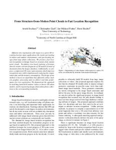
In order to predict the tightening dates we need predictions of the turning points for these three predictor series. Figures 2—4 show the values of these three variables for the most recent cycle. Figure 2 reports the value for the inflation rate based on the GNP deflator.
43
The inflation rate has been quite volatile coming into the third quarter of 2009 but there does appear to be evidence that the rate of decline of the inflation rate is slowing. Thus we will use as the turning point for inflation as 2009Q3 or 0 in terms of the number of quarters after the trough date. Figure 3 shows output gap as measured as percentage deviation from the Hodrick-Prescott filter trend of log real output. It does appear that the output gap has turned, so we will use 2009 Q2 or -1 as the turning point for the output gap. Figure 4 shows the unemployment rate for the most recent cycle. 7 The unemployment rate’s increase is clearly slowing so we will use 2009 Q4 as the turning point for unemployment.
These predicted turning points were then used to generate the predicted tightening dates for the various policy variables. The predicted tightening dates using the individual regressions reflect the differences in turning points in the predictors. Using inflation or unemployment we get predicted tightening dates for the nominal Fed Funds rate or the “narrative” rate between one and two quarters after the trough date, suggesting Fed tightening sometime in early 2010. Using the systems estimates the same picture emerges when using inflation and unemployment as the predictor. The predicted tightening dates for these models range from 1 quarter after the trough date to 2 1/2 quarters after the trough date. The predicted tightening dates for the growth of money base and real money base are much earlier with the modal prediction predicting a tightening on the trough date (2009Q3). This reflects the observation that money base has typically tightened earlier than the nominal policy rates over the post-WWII sample.
7
Note we are not using the most recently revised unemployment data. The decline in the rate of growth of unemployment is even more pronounced using the revised data.
44
The results using the output gap are rather different. Given that the output gap as we have measured it is negative, then the individual regression models predict that tightening should have already occurred. The same holds for the system models with output gap included as a predictor. The predicted tightening date for models using output gap are consistently between one quarter before the trough date or the trough date itself. Given that we have not observed tightening as yet this further suggests that the output gap is not as important as inflation or unemployment in predicting the tightening dates of the policy variables in the post-WWII recessions.
6. Conclusion
This paper presents historical narrative, descriptive, and econometric evidence on the timing of monetary policy in the U.S. after recessions end with respect to the turning points of principal macro-aggregates (but especially unemployment and inflation).We covered 14 business cycles from 1920 to 2007.
In general we find that monetary policy tightens close to when unemployment peaks and when inflation troughs. But that the timing is usually dominated by unemployment. We also find that on a number of occasions that monetary policy measured by the monetary base (real and nominal) shows a different pattern than the official policy interest rates.
45
We found that the timing evidence differed between the interwar period (and in some respects the 1950s) and the post World War II period in a number of respects: First, inflation was not persistent in the interwar (or until the 1960s) so the measure of price stability that mattered most was the price level. In the 1920s and in the 1950s policy tightened when the price level began to rise. Second, in the 1920s (and in the 1950s) tightening occurred when prices rose and before unemployment peaked. We found a few episodes where tightening occurred before recessions ended suggesting that the Fed was following countercyclical policy.
An important fact to note is that since the mid 1960s inflation increased and became persistent for close to 20 years. In those cycles the timing of the tightening doesn’t show that the pace of tightening was not sufficient to reduce the rising trend in inflation. Since the mid 1980s during the Great Moderation although inflation was reduced significantly the timing of policy tightening still favored unemployment.
There are several possible reasons for these patterns: First, in the interwar the Fed followed gold standard orthodoxy which placed primary importance on price stability. Second, after World War II and the Employment Act of 1945, the Fed followed a dual mandate for price stability and high employment. Third, beginning in the 1960s the Fed adhered to Keynesian theories and the Phillips Curve which attached primary importance to low unemployment over low inflation. Fourth, the dominance of unemployment in the timing of tightening in the postwar reflects in addition to Keynesian theory, political pressure by the Congress and the Administration on many occasions to not tighten while
46
unemployment was unacceptably high. Fifth, even in the Great Moderation era since the mid 1980s, after inflation had been significantly reduced and considerable emphasis has been placed on the importance of a credible nominal anchor, the timing of exits favors unemployment. This was evident in the last two cycles. In both cases of jobless recoveries political pressure may have been important.
How will the exit strategy play out for the current cycle? The evidence in Section 5 suggests that if we follow the timing patterns seen in the postwar in the current cycle, and if unemployment peaks in the fourth quarter of 2009, that we may see a tightening in the first quarter of 2010 but more likely in the first half of 2010. Although if unemployment declines slowly from its current elevated level, political pressure and or the Fed’s experience from the last two recessions may stall the tightening longer.
47
Cycle 1. 1920Q1—1923Q1 (1921Q3)a 2. 1923Q2—1926Q2 (1924Q3) 3. 1926Q3—1929Q2 (1927Q4) 4. 1929Q3—1937Q1 (1933Q1)
Table 1a: Descriptive Evidence Policy Variables 1920—1937 Discount Real Discount Base Real Base Narratives Rate Rate Growth Growth
M2 Growth
Real M2 Growth
3b
5
--
5
1
2
2
3
1
2
0
2
-1
2
1
0
0
1
0
0
0
14
--
--
3
3
-2
4
a
Numbers in parentheses are the NBER trough dates for each cycle. Numbers in cells represent number of quarters post official NBER trough date the series was determined to have turned. In the case of the policy variables this date was the date of initial tightening. Missing value represent a cycle in which no definitive turning point was identified. b
Cycle 1. 1920Q1—1923Q1 (1921Q3)a 2. 1923Q2—1926Q2 (1924Q3) 3. 1926Q3—1929Q2 (1927Q4) 4. 1929Q3—1937Q1 (1933Q1)
Table 1b: Descriptive Evidence Macro Aggregates 1920—1937 Price Level Price Level Real Industrial Output (GNP defl.) (CPI) GNP Production Gap
Unemployment
3b
2
-2
-2
-2
-2
0
-2
0
-1
0
-2
-2
1
0
0
0
1
0
0
0
0
0
-4
a
Numbers in parentheses are the NBER trough dates for each cycle. Numbers in cells represent number of quarters post official NBER trough date the series was determined to have turned. In the case of the policy variables this date was the date of initial tightening. Missing value represent a cycle in which no definitive turning point was identified. b
48
Cycle 1. 1948Q4—1953Q1 (1949Q4)a 2. 1953Q2—1957Q2 (1954Q2) 3. 1957Q3—1960Q1 (1958Q2) 4. 1960Q2—1969Q3 (1961Q1) 5. 1969Q4—1973Q3 (1970Q4) 6. 1973Q4—1979Q4 (1975Q1) 7. 1980Q1—1981Q2 (1980Q3) 8. 1981Q3—1990Q2 (1982Q4) 9. 1990Q3—2000Q4 (1991Q1) 10. 2001Q1—2007Q3 (2001Q4)
Table 2a: Descriptive Evidence Policy Variables 1948—2007 Real Fed Funds Fed. Funds Base Real Base Rate Rate Narratives Growth Growth (Real Discount (Discount Rate) Rate)
M2 Growth
Real M2 Growth
-2b
(2)
(6)
-2
-2
1
0
3
2
1
1
1
0
0
1
0
0
-1
-1
-1
-1
1
1
2
2
2
0
-1
1
1
1
0
-2
1
1
0
1
0
0
0
0
0
3
0
0
-1
-1
-1
-1
3
1
-1
0
1
0
0
12
9
9
5
5
-1
0
10
10
5
0
0
3
-1
a
Numbers in parentheses are the NBER trough dates for each cycle. Numbers in cells represent number of quarters post official NBER trough date the series was determined to have turned. In the case of the policy variables this date was the date of initial tightening. Missing value represent a cycle in which no definitive turning point was identified. b
49
Cycle 1. 1948Q4—1953Q1 (1949Q4)a 2. 1953Q2—1957Q2 (1954Q2) 3. 1957Q3—1960Q1 (1958Q2) 4. 1960Q2—1969Q3 (1961Q1) 5. 1969Q4—1973Q3 (1970Q4) 6. 1973Q4—1979Q4 (1975Q1) 7. 1980Q1—1981Q2 (1980Q3) 8. 1981Q3—1990Q2 (1982Q4) 9. 1990Q3—2000Q4 (1991Q1) 10. 2001Q1—2007Q3 (2001Q4) a b
Table 2b: Descriptive Evidence Macro Aggregates 1948—2007 Inflation(GNP) Inflation(CPI) Real Industrial Output (Price Level) (Price Level) GNP Production Gap
Unemployment
0(1)b
-2(1)
0
-2
0
0
0(-2)
1(2)
-1
-1
0
1
-1
0
-1
-1
0
0
-1
0
-1
-1
0
1
-2
0
0
0
0
3
0
0
0
0
0
1
-1
-1
0
-1
0
0
1
0
-1
0
0
0
5
0
0
0
2
6
-1
-1
-1
0
5
7
Numbers in parentheses are the NBER trough dates for each cycle. Numbers in cells represent number of quarters post official NBER trough date the series was determined to have turned. In the case of the policy variables this date was the date of initial tightening.
50
Table 3: Estimates for Slope Coefficient in Equation (2) (Post WWII Sample) Policy Variables Explanatory Real Fed Real Base Real M2 Variables Narratives Fed Funds Funds Base Growth Growth M2 Growth Growth -0.190 0.080 1.480 1.240 -0.710 0.730 1.000 Inflation(GNP) (0.610) (0.400) (0.340) (0.200) (0.120) (0.270) (0.120) [0.36] [ 0.53] [ 0.04] [ 0.02] [ 0.07] [ 0.03] [ 0.00] 1.200 1.000 -0.810 0.930 -0.500 0.190 1.000 Inflation(CPI) (1.210) (1.290) (1.770) (0.720) (0.500) (0.310) (0.390) [ 0.35] [ 0.47] [ 0.66] [ 0.23] [0.34] [ 0.56] [ 0.03] -2.060 -0.330 -0.710 -1.100 -1.210 -0.260 0.620 Real GNP (2.590) (1.610) (1.650) (0.980) (1.220) (0.820) (0.460) [ 0.45] [ 0.84] [ 0.68] [ 0.30] [ 0.35] [0.76] [ 0.22] 2.180 3.510 -0.100 0.890 0.200 0.280 1.000 Ind. Prod. (1.980) (2.570) (1.590) (1.040) (0.630) (0.360) (0.470) [ 0.30] [ 0.21] [ 0.95] [ 0.42] [0.75] [ 0.46] [ 0.07] 0.350 0.340 -0.120 2.190 2.100 1.370 0.480 Output Gap (0.510) (0.480) (0.690) (0.340) (0.430) (0.230) (0.160) [ 0.51] [ 0.50] [ 0.47] [ 0.01] [ 0.00] [ 0.02] [0.07] 0.320 0.010 1.440 1.430 0.710 0.530 0.480 Unemployment (0.330) (0.120) (0.160) (0.280) (0.250) (0.100) (0.100) [ 0.30] [ 0.91] [ 0.00] [ 0.00] [ 0.00] [ 0.07] [0.00]
51
Table 4: Estimates for Slope Coefficient in Equation (2) (Full Sample) Policy Variables Real M2 Policy Real Policy Base Real Base Explanatory Narratives Ratea Rate Growth Growth M2 Growth Growth Variables 0.100 -0.020 0.150 Price Level 0.840 1.120 0.660 0.560 b /Inflation (0.40) (0.20) (0.20) (0.33) (0.45) (0.26) (0.25) (GNP) [ 0.81] [ 0.03] [ 0.93] [ 0.45] [ 0.03] [ 0.03] [ 0.04] -0.560 0.630 -0.160 0.580 -0.120 0.460 0.120 Price Level /Inflation (1.02) (0.62) (1.04) (0.57) (0.54) (0.30) (0.37) (CPI) [ 0.59] [ 0.33] [ 0.88] [ 0.33] [ 0.83] [ 0.15] [ 0.74] -0.940 -0.480 1.990 -1.070 -0.240 -0.850 0.280 Real GNP (1.22) (1.03) (2.46) (0.94) (0.89) (0.63) (0.62) [ 0.46] [ 0.65] [ 0.44] [ 0.28] [ 0.79] [ 0.20] [ 0.66] 1.020 -0.370 -0.500 -0.340 -0.180 0.250 -0.710 Ind. Prod. (1.22) (0.81) (1.37) (0.72) (0.65) (0.45) (0.43) [ 0.42] [ 0.65] [ 0.72] [ 0.65] [ 0.79] [ 0.59] [ 0.12] -0.140 0.090 -0.300 1.480 1.930 4.170 -0.750 Output Gap (0.41) (0.38) (0.23) (0.54) (0.40) (0.50) (0.19) [ 0.74] [ 0.82] [ 0.21] [ 0.02] [ 0.00] [ 0.00] [ 0.00] -0.070 -0.100 1.030 0.990 0.690 0.450 -0.270 Unemployment (0.21) (0.19) (0.34) (0.29) (0.32) (0.07) (0.12) [ 0.76] [ 0.62] [ 0.01] [ 0.01] [ 0.06] [ 0.00] [ 0.05] a.
The policy rate is the Fed Funds rate after 1954 and the discount rate before 1954. For cycles up to and including the cycle ending in 1957Q2 the turning point used is the turning point for the price level. For recessions after 1957Q2 the turning point for inflation is used.
b.
52
Table 6: Slope Coefficient estimates for Equation (3) (Post WWII) {Real FFR, Variable {Narr, FFR} {FFR, Base} Real Base} 0.89 0.60 0.71 0.51 0.87 0.74 Inflation (0.11) (0.18) (0.14) (0.09) (0.17) (0.15) (GNP) [0.00] [0.01] [0.00] [0.00] [0.00] [0.00] 1.85 0.76 0.99 -0.18 0.58 -0.65 Output Gap (0.14) (0.35) (0.17) (0.46) (0.17) (0.64) [0.00] [0.05] [0.00] [0.70] [0.00] [0.32] 1.20 0.94 0.72 0.97 0.46 1.03 Unemployment (0.14) (0.22) (0.08) (0.30) (0.12) (0.41) [0.00] [0.00] [0.00] [0.00] [0.00] [0.02]
Table 7: Slope Coefficient estimates for Equation (3) (Full Sample) {Real Policy Rate, Variable {Narr, Policy Rate} {Policy Rate, Base} Real Base} 0.90 0.85 0.78 0.76 0.85 0.95 Price Level / Inflation (0.46) (0.54) (0.26) (0.23) (0.25) (0.25) (GNP) [0.06] [0.13] [0.00] [0.00] [0.00] [0.00] 1.48 2.80 0.61 1.14 0.33 1.46 Output Gap (0.59) (0.99) (0.34) (0.70) (0.33) (0.64) [0.02] [0.01] [0.08] [0.11] [0.32] [0.03] 0.22 -0.90 0.06 -0.37 -0.16 -0.58 (0.37) (0.62) (0.15) (0.37) (0.16) (0.31) Unemployment [0.56] [0.13] [0.68] [0.32] [0.32] [0.08]
Variable Inflation(GNP) Output Gap Unemployment {Inf, Out Gap} {Inf, Unemp.} {Inf, Out Gap} {Inf, Unemp.} {Inf, Out Gap} {Inf, Unemp.}
Table 8: Predicted Tightening Dates Fed Funds Real Fed Base Narratives Rate Funds Rate Growth 2.63 1.70 0.28 0.39 -0.67 -1.08 -0.91 -0.35 1.91 1.56 0.55 0.03 0.49 2.45
-0.51 1.45 1.01 1.98
Real Base Growth 0.00 -0.31 -0.03
-1.10 -0.14 0.86 1.38
-0.48 0.05
Notes: These predictions are based on predicted turning points for inflation, the output gap, and unemployment of 0, -1 and 1 respectively.
53
Figure 1: Comparison of Turning Points for Unemployment and Inflation with Tightening Dates
Historical Narratives
Fed Funds Rate
15
15
10
10
5
5
0
0
-5
53 57 60 69 73 79 81 90 00 07
-5
53 57 60 69 73 79 81 90 00 07
Quarters before tightening
Real Fed Funds Rate
Money Base Growth
6
4 2
4 0 2
-2 -4
0 -6 -2
53 57 60 69 73 79 81 90 00 07
-8
53 57 60 69 73 79 81 90 00 07
Real Money Base Growth 5
0 Unemployment -5
-10
Inflation (GNP)
53 57 60 69 73 79 81 90 00 07
Year of end of cycle
54
Figure 2: Inflation Rate for most recent Cycle 5
% (annual rate)
4 3 2 1 0 -1
2007Q4 2008Q1 2008Q2 2008Q3 2008Q4 2009Q1 2009Q2 2009Q3 Year and Quarter
Figure 3: Output Gap for most recent Cycle 3 2
% deviation
1 0 -1 -2 -3 -4
2007Q4 2008Q1 2008Q2 2008Q3 2008Q4 2009Q1 2009Q2 2009Q3 Year and Quarter
55
Figure 4: Unemployment Rate for most recent Cycle 10 9
%
8 7 6 5 4
2007Q4 2008Q1 2008Q2 2008Q3 2008Q4 2009Q1 2009Q2 2009Q3 Year and Quarter
56
References
Nathan S. Balke and Robert J. Gordon (1986) “Historical Data” (Appendix B) in Robert J Gordon (ed.) The American Business Cycle: Continuity and Change, NBER Studies in Business Cycles, vol 25, Chicago, Chicago University Press.
Ben Bernanke and Cara Lown (1991) “The Credit Crunch of 1990” Brookings Papers on Economic Activity.
Michael Bordo and Barry Eichengreen (2008), “Bretton Woods and the Great Inflation.” NBER Working Paper 14532
Michael Bordo,Christopher Erceg, Andrew Levin,and Ryan Michaels (2007), “Three Great American Disinflations,” NBER Working Paper 12982
Michael Bordo and Joseph Haubrich (2009), “Credit Crises, Money and Contractions: An Historical View,” NBER Working Paper 15389.
Stijn Claessens, M Ayhan Kose and Marco Terrones (2008), “What Happens during Recessions, Crunches and Busts?” IMF Working Paper 08/274.
57
Hal Cole and Lee Ohanian (2004), “New Deal Policies and the Persistence of the Great Depression: A General Equilibrium Analysis” Journal of Political Economy, Vol. 112(4), pp 779—816.
Gautti Eggertsson (2008), “Great Expectations and the End of the Depression.” American Economic Review, Vol 94( 4), pp. 1476-1516.
Milton Friedman (1953), “The Effects of a Full Employment Policy on Economic Stability; A Formal Analysis.” In Essays in Positive Economics. Chicago: University of Chicago Press.
Milton Friedman and Anna J. Schwartz (1963), A Monetary History of the United States: 1867 to 1960. Princeton: Princeton University Press.
Robert Hetzel ( 2008), The Monetary Policy of the Federal Reserve: A History. New York: Cambridge University Press.
Paul W. Holland and Roy. E. Welsch (1977), "Robust Regression Using Iteratively Reweighted Least-Squares." Communications in Statistics: Theory and Methods, A6, pp. 813–827.
International Monetary Fund (2008) World Economic Outlook
58
Allan Meltzer (2003), A History of the Federal Reserve. Volume I 1913-1951. Chicago: University of Chicago Press.
Allan Meltzer (2010), A History of the Federal Reserve. Volume II 1951-1987. Chicago; University of Chicago Press.( in press)
Michael Mussa (2009), “Global Economic Prospects as of September 2009: Onward to Global Recovery.” Peterson Institute, September.
Carmen Reinhart and Kenneth Rogoff (2009), This Time is Different: Eight Centuries of Financial Folly. Princeton: Princeton University Press
Christina Romer (1992), “What Ended the Great Depression?” Journal of Economic History 52( 4) December pp 757-784.
Christina Romer and David Romer (1994), “Monetary Policy Matters” Journal of Monetary Economics, 34 (August ) pp 75-88.
59
Appendix
A1. Data appendix
Table A1: Data Definitions Variable Discount rate
Source Obtained from the Board of Governors database (H.15). Before 1954 the discount rate is the New York Fed discount rate. The discount rate series is discontinued after 2002 and the Discount Window Primary Credit rate is used after 2002. Monthly data converted to quarterly data using quarterly averages. Federal Funds Rate Effective Federal Funds rate (FEDFUNDS): Obtained from St Louis Fed data base (FRED)a. Monthly data converted to Quarterly data using quarterly averages. Real rate obtained by subtracting inflation rate (computed using GNP deflator). Money Base St Louis adjusted monetary base (seasonally adjusted, AMBSL): Obtained from FRED. Monthly data converted to quarterly data using quarterly averages. Real rate obtained by dividing by GNP deflator. Growth rates are one quarter growth rates expressed as an annualized rate. M2 M2 from Balke and Gordon (1986) until 1983. After 1983 used M2 series from FRED database (seasonally adjusted, M2SL). Monthly data converted to quarterly data using quarterly averages. The two series were spliced at join. Real data obtained by dividing by GNP deflator. Growth rates are one quarter growth rates expressed as an annualized rate. Price Level (GNP) GNP deflator obtained from Balke and Gordon (1986) until 1983. After that used GNP deflator from FRED database (seasonally adjusted, GNPDEF). The two series were spliced at join. Price Level (CPI) Consumer price index for all urban consumers: All items. Obtained from FRED database (CPIAUCNS). Monthly data converted to quarterly data using quarterly averages. Inflation (GNP) Percentage one quarter change in GNP deflator expressed at an annualized rate. Inflation (CPI) Percentage one quarter change in CPI expressed at an annualized rate. Real GNP Real Gross National Product obtained from Balke and Gordon (1986) for periods up until 1983. Afterwards used quarterly GNP data from FRED database (GNP). GNP price deflator from FRED spliced with Balke and Gordon (1986) price deflator. Real GNP after 1983 is nominal GNP divided by spliced GNP deflator series.
60
Industrial Production Unemployment
Output Gap
a.
Obtained from FRED database (INDPRO). Monthly series converted to quarterly series using quarterly averages. Obtained from Bureau of Labor Statistics. Unemployment rate: Civilian Labor Force (LNS14000000, seasonally adjusted). Monthly data converted to quarterly data using quarterly averages. Proportional deviation of real GNP from long-run trend. Computed as the deviations of the logarithm of real GNP from its long-run trend as computed using Hodrick-Prescott filter with smoothing parameter λ =1600.
http://research.stlouisfed.org/fred2/
61
A2. Dates of Turning points of series Table A2-a: Turning Dates: Policy Variables 1920—1937 Cycle 1. 20Q1-23Q1 (1921Q3)a 2. 23Q2-26Q2 (1924Q3) 3. 26Q3-29Q2 (1927Q4) 4. 29Q3-37Q1 (1933Q1)
Narratives
Discount Rate
Real Discount Rate
Base Growth
Real Base Growth
M2 Growth
Real M2 Growth
1922Q2
1922Q4
--
1922Q4
1921Q4
1922Q1
1922Q1
1925Q2
1924Q4
1925Q1
1924Q3
1925Q1
1924Q2
1925Q1
1928Q1
1927Q4
1927Q4
1928Q1
1927Q4
1927Q4
1927Q4
1936Q3
--
--
1933Q4
1933Q4
1932Q3
1934Q1
a
Dates in parentheses are the NBER trough dates for each cycle. Missing value represent a cycle in which no definitive turning point was identified.
Table A2-b: Turning Dates: Macro Aggregates 1920—1937 Cycle 1. 20Q1-23Q1 (1921Q3)a 2. 23Q2-26Q2 (1924Q3)
a
Price Level Price Level (GNP deflator.) (CPI)
Real GNP
Industrial Production
Output Gap
Unemployment
1922Q2
1922Q1
1921Q1
1921Q1
1921Q1
1921Q1
1924Q3
1924Q1
1924Q3
1924Q2
1924Q3
1924Q1
3. 26Q3-29Q2 (1927Q4)
1927Q2
1928Q1
1927Q4
1927Q4
1927Q4
1928Q1
4. 29Q3-37Q1 (1933Q1)
1933Q1
1933Q1
1933Q1
1933Q1
1933Q1
1932Q1
Dates in parentheses are the NBER trough dates for each cycle.
62
Table A3-a: Turning Dates: Policy Variables 1948—2007
Cycle 1. 48Q4-53Q1 (1949Q4)a 2. 53Q2-57Q2 (1954Q2)
a
Fed. Funds Rate (Discount Narratives Rate)
Real Fed Funds Rate (Real Discount Rate)
Base Real Base M2 Real M2 Growth Growth Growth Growth
1949Q2
(1950Q2)
(1951Q1)
1949Q2
1949Q2
1950Q1 1949Q4
1955Q1
1954Q4
1954Q3
1954Q3
1954Q3
1954Q2 1954Q2
3. 57Q3-60Q1 (1958Q2)
1958Q3
1958Q2
1958Q2
1958Q1
1958Q1
1958Q1 1958Q1
4. 60Q2-69Q3 (1961Q1)
1961Q2
1961Q2
1961Q3
1961Q3
1961Q3
1961Q1 1960Q4
5. 69Q4-73Q3 (1970Q4)
1971Q1
1971Q1
1971Q1
1970Q4
1970Q2
1971Q1 1971Q1
6. 73Q4-79Q4 (1975Q1)
1975Q1
1975Q2
1975Q1
1975Q1
1975Q1
1975Q1 1975Q1
7. 80Q1-81Q2 (1980Q3)
1981Q2
1980Q3
1980Q3
1980Q2
1980Q2
1980Q2 1980Q2
8. 81Q3-90Q2 (1982Q4)
1983Q3
1983Q1
1982Q3
1982Q4
1983Q1
1982Q4 1982Q4
9. 90Q3-00Q4 (1991Q1)
1994Q1
1993Q2
1993Q2
1992Q2
1992Q2
1990Q4 1991Q1
10. 01Q1-07Q3 (2001Q4)
2004Q2
2004Q2
2003Q1
2001Q4
2001Q4
2002Q3 2001Q3
Dates in parentheses are the NBER trough dates for each cycle.
63
Table 2b: Turning Dates: Macro Aggregates 1948—2007
a
Cycle
Inflation(GNP) (Price Level)
Inflation(CPI) (Price Level)
Real GNP
Industrial Production
Output Gap
Unemployment
1. 48Q4-53Q1 (1949Q4)a
1949Q4 (1950Q1)
1949Q2 (1950Q1)
1949Q4
1949Q2
1949Q4
1949Q4
2. 53Q2-57Q2 (1954Q2)
1954Q2 (1953Q4)
1954Q3 (1954Q4)
1954Q1
1954Q1
1954Q2
1954Q3
3. 57Q3-60Q1 (1958Q2)
1958Q1
1958Q2
1958Q1
1958Q1
1958Q2
1958Q2
4. 60Q2-69Q3 (1961Q1)
1960Q4
1961Q1
1960Q4
1960Q4
1961Q1
1961Q2
5. 69Q4-73Q3 (1970Q4)
1970Q2
1970Q4
1970Q4
1970Q4
1970Q4
1971Q3
6. 73Q4-79Q4 (1975Q1)
1975Q1
1975Q1
1975Q1
1975Q1
1975Q1
1975Q2
7. 80Q1-81Q2 (1980Q3)
1980Q2
1980Q2
1980Q3
1980Q2
1980Q3
1980Q3
8. 81Q3-90Q2 (1982Q4)
1983Q1
1982Q4
1982Q3
1982Q4
1982Q4
1982Q4
9. 90Q3-00Q4 (1991Q1)
1984Q1
1991Q1
1991Q1
1991Q1
1991Q3
1984Q2
10. 01Q1-07Q3 (2001Q4)
2001Q3
2001Q3
2001Q3
2001Q4
2003Q1
2003Q7
Date in parentheses are the NBER trough dates for each cycle.
64
A3. Figures of Data and Turning Points Figure A1: Nominal Discount Rate
1920Q1-1923Q1
1923Q2-1926Q2
8
5
6
4
4 -10
-5
0 5 1926Q3-1929Q2
10
3 -5
5
10
4
5
3 -5
0 5 1948Q4-1953Q1
10
2
0 -20
0 5 1929Q3-1937Q1
10
-10
0 10 1953Q2-1957Q2
20
0
5 10 1960Q2-1969Q3
15
0
10 20 1973Q4-1979Q4
30
40
0
5 10 1981Q3-1990Q2
15
20
3
1.8
2
1.6 -5
0
5 10 1957Q3-1960Q1
15
1 -5
4
6
2
4
0 -5
0 5 1969Q4-1973Q3
10
2 -10
8
15
6
10
4 -5
0
5 10 1980Q1-1981Q2
15
5 -5
14
15
12
10
10 -2
-1
0 1 1990Q3-2000Q4
2
3
5 -10
10
10
5
5
0 -10
0
10
20
30
40
0 -10
0
0
10 20 2001Q1-2007Q3
10
20
30
30
65
Figure A2: Federal Funds Rate
1953Q2-1957Q2
1957Q3-1960Q1
4
4
2
2
0 -5
0
5
10
15
0 -5
0
1960Q2-1969Q3 20
5
10
0
10
20
30
40
0 -5
0
1973Q4-1979Q4 20
10
10
0
5
10
15
20
0 -2
-1
1981Q3-1990Q2 10
10
5
0
10
10
15
0
1
2
3
30
40
1990Q3-2000Q4
20
0 -10
5 1980Q1-1981Q2
20
0 -5
10
1969Q4-1973Q3
10
0 -10
5
20
30
20
30
0 -10
0
10
20
2001Q1-2007Q3 10
5
0 -10
0
10
66
Figure A3: Real Discount Rate
1920Q1-1923Q1
1923Q2-1926Q2
20
5
0 -20 -10
-5
0 5 1926Q3-1929Q2
10
0 -5
6
20
5
0
4 -5
0 5 1948Q4-1953Q1
10
-20 -20
10
5
0
0
-10 -5
0
5 10 1957Q3-1960Q1
15
4
0
2
0 5 1969Q4-1973Q3
10
0 -10
2
5
0
0
-2 -5
0
5 10 1980Q1-1981Q2
15
-5 -5
5
10
0
5
-5 -2
-1
0 1 1990Q3-2000Q4
2
3
0 -10
5
5
0
0
-5 -10
0
10
20
30
40
10
-10
0 10 1953Q2-1957Q2
20
0
5 10 1960Q2-1969Q3
15
0
10 20 1973Q4-1979Q4
30
40
0
5 10 1981Q3-1990Q2
15
20
-5 -5
5
-5 -5
0 5 1929Q3-1937Q1
-5 -10
0
0
10 20 2001Q1-2007Q3
10
20
30
30
67
Figure A4: Real Federal Funds Rate
1953Q2-1957Q2
1957Q3-1960Q1
5
5
0
0
-5 -5
0
5
10
15
-5 -5
0
1960Q2-1969Q3 5
2
0
0
10
20
30
40
-5 -5
0
1973Q4-1979Q4 10
0
0
0
5
10
15
20
-10 -2
-1
1981Q3-1990Q2 5
5
0
0
10
10
15
0
1
2
3
30
40
1990Q3-2000Q4
10
0 -10
5 1980Q1-1981Q2
5
-5 -5
10
1969Q4-1973Q3
4
0 -10
5
20
30
20
30
-5 -10
0
10
20
2001Q1-2007Q3 5
0
-5 -10
0
10
68
Figure A5: Base Growth
1920Q1-1923Q1
1923Q2-1926Q2
20
10
0
0
-20 -10
-5
0 5 1926Q3-1929Q2
10
-10 -5
5
100
0
0
-5 -5
0 5 1948Q4-1953Q1
10
-100 -20
20
5
0
0
-20 -5
0
5 10 1957Q3-1960Q1
15
10
0
5
0 5 1969Q4-1973Q3
10
0 -10
20
20
10
10
0 -5
0
5 10 1980Q1-1981Q2
15
0 -5
20
20
10
10
0 -2
-1
0 1 1990Q3-2000Q4
2
3
0 -10
50
50
0
0
-50 -10
0
10
20
30
40
10
-10
0 10 1953Q2-1957Q2
20
0
5 10 1960Q2-1969Q3
15
0
10 20 1973Q4-1979Q4
30
40
0
5 10 1981Q3-1990Q2
15
20
-5 -5
10
-10 -5
0 5 1929Q3-1937Q1
-50 -10
0
0
10 20 2001Q1-2007Q3
10
20
30
30
69
Figure A6: Real Base Growth
1920Q1-1923Q1
1923Q2-1926Q2
50
20
0
0
-50 -10
-5
0 5 1926Q3-1929Q2
10
-20 -5
20
100
0
0
-20 -5
0 5 1948Q4-1953Q1
10
-100 -20
10
5
0
0
-10 -5
0
5 10 1957Q3-1960Q1
15
10
0
0
0 5 1969Q4-1973Q3
10
-10 -10
10
50
0
0
-10 -5
0
5 10 1980Q1-1981Q2
15
-50 -5
10
20
0
0
-10 -2
-1
0 1 1990Q3-2000Q4
2
3
-20 -10
50
50
0
0
-50 -10
0
10
20
30
40
10
-10
0 10 1953Q2-1957Q2
20
0
5 10 1960Q2-1969Q3
15
0
10 20 1973Q4-1979Q4
30
40
0
5 10 1981Q3-1990Q2
15
20
-5 -5
5
-5 -5
0 5 1929Q3-1937Q1
-50 -10
0
0
10 20 2001Q1-2007Q3
10
20
30
30
70
Figure A7: M2 Growth
1920Q1-1923Q1
1923Q2-1926Q2
20
20
0
10
-20 -10
-5
0 5 1926Q3-1929Q2
10
0 -5
10
50
0
0
-10 -5
0 5 1948Q4-1953Q1
10
-50 -20
10
10
0
5
-10 -5
0
5 10 1957Q3-1960Q1
15
20
5
10
0 5 1969Q4-1973Q3
10
0 -10
20
20
10
0
0 -5
0
5 10 1980Q1-1981Q2
15
-20 -5
20
40
10
20
0 -2
-1
0 1 1990Q3-2000Q4
2
3
0 -10
20
20
0
0
-20 -10
0
10
20
30
40
10
-10
0 10 1953Q2-1957Q2
20
0
5 10 1960Q2-1969Q3
15
0
10 20 1973Q4-1979Q4
30
40
0
5 10 1981Q3-1990Q2
15
20
0 -5
10
0 -5
0 5 1929Q3-1937Q1
-20 -10
0
0
10 20 2001Q1-2007Q3
10
20
30
30
71
Figure A8: Real M2 Growth
1920Q1-1923Q1
1923Q2-1926Q2
50
20
0
10
-50 -10
-5
0 5 1926Q3-1929Q2
10
0 -5
20
50
0
0
-20 -5
0 5 1948Q4-1953Q1
10
-50 -20
10
10
0
0
-10 -5
0
5 10 1957Q3-1960Q1
15
10
0
0
0 5 1969Q4-1973Q3
10
-10 -10
20
50
0
0
-20 -5
0
5 10 1980Q1-1981Q2
15
-50 -5
10
20
0
0
-10 -2
-1
0 1 1990Q3-2000Q4
2
3
-20 -10
10
10
0
0
-10 -10
0
10
20
30
40
10
-10
0 10 1953Q2-1957Q2
20
0
5 10 1960Q2-1969Q3
15
0
10 20 1973Q4-1979Q4
30
40
0
5 10 1981Q3-1990Q2
15
20
-10 -5
10
-10 -5
0 5 1929Q3-1937Q1
-10 -10
0
0
10 20 2001Q1-2007Q3
10
20
30
30
72
Figure A9: Price Level (GNP deflator)
1920Q1-1923Q1
1923Q2-1926Q2
50
34
40
33
30 -10
-5
0 5 1926Q3-1929Q2
10
32 -5
34
40
33
30
32 -5
0 5 1948Q4-1953Q1
10
20 -20
60
65
55
60
50 -5
0
5 10 1957Q3-1960Q1
15
70
0 5 1929Q3-1937Q1
10
-10
0 10 1953Q2-1957Q2
20
0
5 10 1960Q2-1969Q3
15
0
10 20 1973Q4-1979Q4
30
40
0
5 10 1981Q3-1990Q2
15
20
55 -5 100
68
80
66 -5
0 5 1969Q4-1973Q3
10
60 -10
120
200
100
150
80 -5
0
5 10 1980Q1-1981Q2
15
100 -5
200
300
180
200
160 -2
-1
0 1 1990Q3-2000Q4
2
3
100 -10
350
400
300
350
250 -10
0
10
20
30
40
300 -10
0
0
10 20 2001Q1-2007Q3
10
20
30
30
73
Figure A10: Price Level (CPI)
1920Q1-1923Q1
1923Q2-1926Q2
20
18
18
17.5
16 -10
-5
0 5 1926Q3-1929Q2
10
17 -5
18
20
17.5
15
17 -5
0 5 1948Q4-1953Q1
10
10 -20
30
30
25
28
20 -5
0
5 10 1957Q3-1960Q1
15
40
29
30
0 5 1969Q4-1973Q3
10
20 -10
45
80
40
60
35 -5
0
5 10 1980Q1-1981Q2
15
40 -5
90
150
80
100
70 -2
-1
0 1 1990Q3-2000Q4
2
3
50 -10
200
250
150
200
100 -10
0
10
20
30
40
10
-10
0 10 1953Q2-1957Q2
20
0
5 10 1960Q2-1969Q3
15
0
10 20 1973Q4-1979Q4
30
40
0
5 10 1981Q3-1990Q2
15
20
26 -5
30
28 -5
0 5 1929Q3-1937Q1
150 -10
0
0
10 20 2001Q1-2007Q3
10
20
30
30
74
Figure A11: Inflation (GNP deflator)
1920Q1-1923Q1
1923Q2-1926Q2
50
10
0
0
-50 -10
-5
0 5 1926Q3-1929Q2
10
-10 -5
10
50
0
0
-10 -5
0 5 1948Q4-1953Q1
10
-50 -20
20
5
0
0
-20 -5
0
5 10 1957Q3-1960Q1
15
10
2
0
0 5 1969Q4-1973Q3
10
-10 -10
10
20
5
10
0 -5
0
5 10 1980Q1-1981Q2
15
0 -5
15
10
10
5
5 -2
-1
0 1 1990Q3-2000Q4
2
3
5
0 -10
10
-10
0 10 1953Q2-1957Q2
20
0
5 10 1960Q2-1969Q3
15
0
10 20 1973Q4-1979Q4
30
40
0
5 10 1981Q3-1990Q2
15
20
-5 -5
4
0 -5
0 5 1929Q3-1937Q1
0 -10
0
10 20 2001Q1-2007Q3
30
5
0
10
20
30
40
0 -10
0
10
20
30
75
Figure A12: Inflation (CPI)
1920Q1-1923Q1
1923Q2-1926Q2
20
5
0
0
-20 -10
-5
0 5 1926Q3-1929Q2
10
-5 -5
0
20
-2
0
-4 -5
0 5 1948Q4-1953Q1
10
-20 -20
20
5
0
0
-20 -5
0
5 10 1957Q3-1960Q1
15
10
0
0
0 5 1969Q4-1973Q3
10
-10 -10
20
20
10
10
0 -5
0
5 10 1980Q1-1981Q2
15
0 -5
15
10
10
0
5 -2
-1
0 1 1990Q3-2000Q4
2
3
-10 -10
10
10
5
0
0 -10
0
10
20
30
40
10
-10
0 10 1953Q2-1957Q2
20
0
5 10 1960Q2-1969Q3
15
0
10 20 1973Q4-1979Q4
30
40
0
5 10 1981Q3-1990Q2
15
20
-5 -5
5
-5 -5
0 5 1929Q3-1937Q1
-10 -10
0
0
10 20 2001Q1-2007Q3
10
20
30
30
76
Figure A13: Real GNP
1920Q1-1923Q1
1923Q2-1926Q2
300
300
200
250
100 -10
-5
0 5 1926Q3-1929Q2
10
200 -5
350
400
300
300
250 -5
0 5 1948Q4-1953Q1
10
200 -20
1000
800
500
700
0 -5
0
5 10 1957Q3-1960Q1
15
1500
700
1000
0 5 1969Q4-1973Q3
10
500 -10
1400
2000
1200
1500
1000 -5
0
5 10 1980Q1-1981Q2
15
1000 -5
1650
2500
1600
2000
1550 -2
-1
0 1 1990Q3-2000Q4
2
3
1500 -10
4000
4000
3000
3500
2000 -10
0
10
20
30
40
10
-10
0 10 1953Q2-1957Q2
20
0
5 10 1960Q2-1969Q3
15
0
10 20 1973Q4-1979Q4
30
40
0
5 10 1981Q3-1990Q2
15
20
600 -5
800
600 -5
0 5 1929Q3-1937Q1
3000 -10
0
0
10 20 2001Q1-2007Q3
10
20
30
30
77
Figure A14: Industrial Production
1920Q1-1923Q1
1923Q2-1926Q2
8
8
6
6
4 -10
-5
0 5 1926Q3-1929Q2
10
4 -5
9
10
8
5
7 -5
0 5 1948Q4-1953Q1
10
25
0 -20
0 5 1929Q3-1937Q1
10
-10
0 10 1953Q2-1957Q2
20
0
5 10 1960Q2-1969Q3
15
0
10 20 1973Q4-1979Q4
30
40
0
5 10 1981Q3-1990Q2
15
20
25
20 15 -5
0
5 10 1957Q3-1960Q1
15
20 -5
30
60
25
40
20 -5
0 5 1969Q4-1973Q3
10
20 -10
60
60
50
50
40 -5
0
5 10 1980Q1-1981Q2
15
40 -5
58
80
56
60
54 -2
-1
0 1 1990Q3-2000Q4
2
3
40 -10
150
120
100
100
50 -10
0
10
20
30
40
80 -10
0
0
10 20 2001Q1-2007Q3
10
20
30
30
78
Figure A15: Output Gap
1920Q1-1923Q1
1923Q2-1926Q2
0.2
0.1
0
0
-0.2 -10
-5
0 5 1926Q3-1929Q2
10
-0.1 -5
0.2
0.2
0
0
-0.2 -5
0 5 1948Q4-1953Q1
10
-0.2 -20
0.1
0.05
0
0
-0.1 -5
0
5 10 1957Q3-1960Q1
15
0.05
0
0
0 5 1969Q4-1973Q3
10
-0.05 -10
0.05
0.05
0
0
-0.05 -5
0
5 10 1980Q1-1981Q2
15
-0.05 -5
0.05
0.05
0
0
-0.05 -2
-1
0 1 1990Q3-2000Q4
2
3
-0.05 -10
0.05
0.05
0
0
-0.05 -10
0
10
20
30
40
10
-10
0 10 1953Q2-1957Q2
20
0
5 10 1960Q2-1969Q3
15
0
10 20 1973Q4-1979Q4
30
40
0
5 10 1981Q3-1990Q2
15
20
-0.05 -5
0.05
-0.05 -5
0 5 1929Q3-1937Q1
-0.05 -10
0
0
10 20 2001Q1-2007Q3
10
20
30
30
79
Figure A16: Unemployment
1920Q1-1923Q1
1923Q2-1926Q2
20
6
10
4
0 -10
-5
0 5 1926Q3-1929Q2
10
2 -5
6
40
4
20
2 -5
0 5 1948Q4-1953Q1
10
0 -20
10
6
5
4
0 -5
0
5 10 1957Q3-1960Q1
15
10
6
5
0 5 1969Q4-1973Q3
10
0 -10
10
10
5
5
0 -5
0
5 10 1980Q1-1981Q2
15
0 -5
8
15
7
10
6 -2
-1
0 1 1990Q3-2000Q4
2
3
5 -10
10
8
5
6
0 -10
0
10
20
30
40
10
-10
0 10 1953Q2-1957Q2
20
0
5 10 1960Q2-1969Q3
15
0
10 20 1973Q4-1979Q4
30
40
0
5 10 1981Q3-1990Q2
15
20
2 -5
8
4 -5
0 5 1929Q3-1937Q1
4 -10
0
0
10 20 2001Q1-2007Q3
10
20
30
30
80