Journal of Sports Sciences, 2003, 21, 479–491

From the cradle to the grave: how fast can we run? ELMER STERKEN* Department of Economics, University of Groningen, PO Box 800, 9700 AV Groningen, The Netherlands

Accepted 7 January 2003

I model average running speed on distances from 5000 m to the marathon as a function of age, distance and sex. Using data on US age-dependent road-racing records, I simulate optimal performance for ages ranging from 3 to 95 years. The results of the correlation between running speed and age are in line with medical results on the relation between age and maximal oxygen uptake. The results show that official track and field age-grading overestimates human performance at older ages. Keywords: performance, endurance, running speed.

Introduction The statistical analysis of sport performance is popular but troublesome (Atkinson and Nevill, 2001). There are many caveats, especially if one wants to analyse the alleged impact of, for instance, training methods or drugs on sport performance. In this paper, I follow an alternative approach and start from a precise measurement of performance and subsequently describe its determinants. I model long-distance average running speed V (V = DIST/T, where DIST is the race distance in metres and T is the time to run distance DIST in seconds) as a function of age (AGE, measured in years), distance (DIST) and sex (G = 1 for men and 0 for women). These results are compared with medical findings about the relationship between maximal oxygen uptake and age and official track and field tables used to correct individual performances for age. The main focus of this paper is on the relationship between average running speed and age. We know with certainty that babies and dead people can’t run. But how does long-distance running performance develop during our lifetime? As teenagers we make substantial progress, but it is unavoidable that we slow down after a certain age. At what age do we perform optimally and how fast do we slow down? There are some basic notions about the impact of ageing on running performance. For instance, the World Masters Athletes (WMA), formerly the World Association of Veteran Athletes (WAVA), publishes age-group dependent correction factors. These correc-

* e-mail: [email protected].

tion factors are used to grade results in track and field and road-racing events. One of the serious flaws of the WMA data is the rather arbitrary subdivision of ages into age classes (of 5 years). The aim here is to present more precise cross-event, cross-sex estimates of correction factors. The WMA tables probably also overestimate the capabilities of very old runners (Fair, 1994). Using a statistical model, I simulate ‘normal’ values for average speed depending on age, various distances (varying from 5000 to 42,195 m) and sex. These ‘normal’ values can be compared with the official age-grading tables. I use long-distance running data to analyse the impact of ageing on endurance, because these data are age-specific and publicly available. I include data on US record times for distances between 5000 and 42,195 m (the marathon) for men and women aged 3–95 years. It is known that the average running speed observed in road-racing events suffers from measurement error. Therefore, I compute the ‘normal’ values based on smoothing out measurement errors in the data via ordinary least squares. In the next section, I present the basic theoretical notions for modelling average running speed V. In particular, I discuss the impact of age and distance on running speed. I do not derive a formal model, but present some plausible physiological assumptions in explaining V. I then introduce the data and provide some basic descriptive statistics. Following this, I present the model that predicts the optimal speed based on age, distance and sex. Moreover, I present various robustness checks on the results and compare the results with findings presented in the literature. Finally, I provide a summary and present my conclusions.

Journal of Sports Sciences ISSN 0264-0414 print/ISSN 1466-447X online # 2003 Taylor & Francis Ltd DOI: 10.1080/0264041031000101791

480 Theory The maximal running speed in anaerobic events (such as the 100 m dash) depends on the muscular structure of the body. The physiological differences in muscular strength between women and men determine to a large extent the differences in results between the sexes. It is known, for instance, that in sprint events women require a longer distance to reach their maximal instantaneous running speed: 67 m for women versus 50 m for men (Grubb, 1998). It is also clear that in sprint events there are wide differences in running speed during the event. This fact makes it troublesome to use average running speed V as an indicator of performance. In aerobic events, such as the marathon, endurance is the most prominent physical characteristic. Here it is the ability of the body to transport oxygen to the muscles (mostly described by maximal oxygen intake or V_ O2max) that plays a key role. Again the differences in muscular structure between women and men allow men to run faster. Differences in running speed between the sexes during the events are smaller though (Grubb, 1998). The aerobic events are also characterized by the notion that a constant running speed is optimal during races over distances of more than 800 m (Keller, 1974), which allows us to use average running speed V as a performance indicator. I focus on the lower bounds of running time T (Blest, 1996) and thus the human performance frontier. This implies that we should analyse average running speed V given perfect race conditions, the use of optimal training methods and the best equipment possible, and perhaps more importantly, the mental ability of the athlete to compete. Fair (1994) postulated a relationship between the lower bound of running time T and age as depicted in Fig. 1. The lower bound is infinite for small babies, falls until a certain age, remains constant

Fig. 1. Postulated relation between the lower bound of a density plot of running times and age.

Sterken (between age h and j) and then starts to rise. Fair was interested in the latter stage and assumed a rather modest linear incline from age j up to age k, whereafter the increase is assumed to be quadratic. Fair estimated this age k for men using only age-specific data for both running and field events. For various models, Fair observed that 47–48 years appears to be the critical age. Moreover, Fair concluded that the rate of physical deterioration of the human body is slow, but faster than the WMA would have us believe. This implies that official age-correction factors, such as those used by the WMA or those available via the Masters Age-Graded Tables (see Mundle et al., 1989), do not favour older runners. Without concerning ourselves too much about physiology, why would we expect a pattern as shown in Fig. 1? The growth of the body, muscles and hormones increases running performance during our youth. Using specific training methods, athletes are able to increase their natural maximal oxygen uptake. After a certain age, maximal oxygen uptake decreases. Fair referred to studies that reported results for ages between 40 and 70 years. Although the estimates vary, a decline of 0.5–0.9% per year seems to be a meta-outcome (see Dehn and Bruce, 1972; Heath et al., 1981; Rogers et al., 1990). For ages close to 40, the lower figure applies, while the decline is larger for older people. Apart from age, I use variation in distances to assess the relation between running speed and both age and sex. Riegel (1981) and Blest (1996) used a log-linear model, log(T) = a +b log(DIST) to fit world records, where T is the running time in seconds and DIST is the distance in metres. Normal values for a are around –2.7 and for b around 1.1. This model can also be formulated in terms of speed: log(V) = 7a +(1 7 b)log (DIST), where V is the average running speed in metres per second. Grubb (1998) used this model and found common values of b for both men and women. Francis (1943) proposed the following model: V = C +A/(log(DIST) 7B), where C is the speed at very long distances, exp(B) is the asymptote of the distance where the maximum speed can be observed and A is a measure of the decrease in speed as distance increases. For this model, Grubb (1998) concluded that female runners have a lower long-distance speed C, but also a slightly lower rate of slowing down A. Keller (1974) estimated B, the turning point for anaerobic to aerobic effort, to be 291 m (so by using long-distance data we can be sure to analyse aerobic events). Another aspect of the model presented here is the joint impact of age and distance on V. Do older runners perform relatively better in long-distance events? In professional athletics, older runners switch from the 1500 to 3000 or 5000 m events, and 10,000 m runners to the half marathon and marathon. The ability to run

481

Running speed throughout life at high average speed appears to decline with age, while endurance can be stimulated and intensified by training. Fair (1994) found evidence for the age–distance hypothesis for men aged 35–70 years. After 70 years of age, performances at long distances appear to slow down relatively quickly. This implies that a distance correction must be age-dependent. More simple analyses of differences between running times by an age-independent factor [as described by, for example, Robinson and Tawn (1995) for the 3000 and 1500 m, where the ratio of the times for 3000 to 1500 m is around 2.16] must, therefore, be interpreted with care. Here, I follow Fair’s (1994) modelling strategy to a large extent. I use his postulated relation between average running speed V and age. The present study has a different purpose though. I analyse only longdistance running data. Fair also analysed field events such as the long jump and pole vault. Because these events focus on muscular strength and we are only interested here in endurance, I do not include field events in the analysis. Moreover, I analyse average running speed for men and women, whereas Fair only studied men. By doing this, I was able to use more data and test for similarities between men and women. Another difference with Fair’s study is that I analyse lifetime development, whereas Fair restricted himself to ages over 35. Since Fair was interested in the mysterious age at which a serious decline in the male body begins, he used a special frontier estimation method to estimate the curve of Fig. 1. I take another approach and consider the contour of Fig. 1 to contain measurement error. With that in mind, I test whether we can combine data from the various events for both women and men, since the literature shows that the male and female contours have similar shapes across distances and sex.

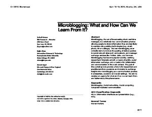
therefore start the analysis by observing actual records per age and distance. I used data from the US-based Long Distance Running Association (2001), an association that keeps records of road-racing events over various distances in the USA. For each age, the fastest time ever ran by an American citizen is recorded with the name, sex and date of birth of the runner, as well as the name and date of the race. Moreover, the set contains information on special conditions of the event (downhill track, wind, etc.) and presents corrected data if necessary. The following distances are recorded: 5000, 8045 (5 miles), 10,000, 12,000, 15,000, 16,090, 20,000, 21,097.5 (half marathon), 25,000, 30,000, 42,195 (marathon) and 80,450 m (50 miles). The recorded ages vary from 3 to 95 years. Figure 2 provides an overview of the nature of the data. It plots the average running speed (vertical axis) of women of various ages (horizontal axis) for the marathon. This figure shows two lines: MARV for the raw data and HMARATV for the so-called filtered series (I use the Hodrick-Prescott filter; see Hodrick and Prescott, 1997). Figure 2 shows a pattern that can be observed in the plots of age-dependent speeds of other distances for both women and men. Figure 2 also presents information about another feature of the data: measurement error of the true underlying, but unobserved, human average running speed function of age. There are various reasons to believe that measurement error is present in the data. Individual strong performance can distort the general pattern. Moreover, for very young and very old ages (say below 10 and above 75 years), there are only a few observations. Because we are interested here in the general development of human endurance, we require series without

In athletics, there is a tradition for measuring the effects of ageing. Various athletic organizations publish agegraded records (see Mundle et al., 1989), which are used by race officials in age-graded events. The WMA published the first set of data in 1989 and provides an update every 5 years. The set contains data for both outdoor and indoor records for men and women for various events ranging from the 100 m to one-hour runs (also for various field events). The WMA data provide records per 5-year age class. The Masters AgeGraded Tables (MAGT) present similar information for track events. One of the disadvantages of both sets is that it is unclear how the tables are compiled. Moreover, as Fair (1994) argued, the official age-graded tables appear to be biased against older runners. I

Speed (m·s–1)

Data

Age (years)

Fig. 2. Average running speed of women of different ages for the marathon. MARV (solid line) represents the raw running speed data; HMARATV (dashed line) represents the filtered data (using the Hodrick-Prescott filter).

482

Sterken

Modelling running speed In this section, I present a statistical analysis of the relationship between average running speed V and age (AGE), distance (DIST) and sex (G). I use all the available information to derive a theoretical prediction of running speed of a female or male runner of a certain age over a specific distance. The data are smoothed to cope with measurement error. Figure 3 presents a contour plot of the running speed data for men. The events are ordered along the inward axis (distances in metres), age (in years) along the horizontal axis and average running speed (in metres per second) along the vertical axis. First, using the econometric software package EVIEWS version 3.1 (Quantitative Micro Software, 1999), I estimate an nth-order polynomial for all events for men and women separately. The dependent variable is average running speed V and the independent variables are: age (AGE), its higher-order terms (AGEi),

distance (DIST) and its higher-order terms (DISTi). I tested for the inclusion of higher-order terms one at a time: this resulted in a fifth-order polynomial in age and distance. Table 1 presents the results for the models for both men and women. In the first column, the independent variables are denoted. AGEDIST is the product of age and distance and AGE2DIST is the squared value of age multiplied by distance. N denotes the number of observations used and SSR is the sum of squared residuals, a measure of the goodness-of-fit of the model. The second and third columns present the

–1 Speed (m·s )

measurement error. We can solve this problem in two ways. First, as is done in Fig. 2, we can smooth the individual series and compute ‘normal’ values. However, this method does not exploit all available information. The alternative method uses all the data (for all events and possibly for both men and women) and therefore contains more information. This latter pooling method is used in the next section.

Di st

an

ce

Ag

(m )

e(

yea

rs)

Fig. 3. Contour plot of men’s average running speed. Source: USA Track and Field Distance Running, www.usaldr.org.

Table 1. Determinants of average running speed by sex (dependent variable: average running speed V, m × s71) Men

Women

Determinant

Coefficient

t-statistic

Coefficient

t-statistic

AGE AGE2 AGE3 AGE4 AGE5 DIST DIST2 DIST3 DIST4 DIST5 AGEDIST AGE2DIST C N SSR

0.362850 70.011068 0.000123 73.37E-07 71.76E-09 70.216063 0.017722 70.000768 1.42E-05 78.84E-08 0.000590 75.71E-06 2.845860 939 37.921

14.79284 78.209404 3.722053 70.915005 71.148809 76.573045 5.586313 75.899633 6.251469 76.510774 5.105083 74.963723 16.44872

0.232424 70.006412 5.59E-05 75.19E-08 71.21E-09 70.193853 0.016143 70.000735 1.41E-05 78.97E-08 0.000605 75.40E-06 3.338996 895 34.954

10.17093 75.028293 1.774895 70.146970 70.823512 76.349411 5.392797 75.941430 6.497409 76.897610 3.655274 73.530442 18.14745

Note: AGE = age (years); AGEi = AGE to the power i; DIST = distance (in kilometres); DISTi = distance to the power i; AGEDIST = age*distance; AGE2DIST = (age)2*distance; C = the intercept. The standard errors are White heteroscedasticity corrected. N = number of observations, SSR = sum of squared residuals.

483

Running speed throughout life estimated coefficients and corresponding t-values for men; columns 4 and 5 give the corresponding results for women. The table shows that the results are similar for men and women. There is no basic difference in the shape of the polynomial. Therefore, I use a pooled model for both men and women and use fixed effects for sex G. In this pooled model, I assume that the shape of the function estimated is identical for both men and women. The only difference is the intercept: there is a constant difference between the running speed of men and women. Table 2 presents the results of this pooled model. This table includes a description of the independent variables (as in Table 1) in the first column. The second column includes the estimated parameters of the pooled model. The third column includes the corresponding t-values. The F-test on pooling the model equals 0.40, which justifies pooling. I now examine the pooled set for the interaction between age, distance and sex. Table 3 presents the model that gives the best statistical fit. The structure of this table is identical to the structure of Tables 1 and 2. The first column includes the headers of the independent variables (see also the table footnotes for a description of the symbols). The second and third columns include the estimated parameters and the corresponding t-statistics. There are significant interactive terms between age and distance, between age and

Table 2. Pooled model of average running speed (dependent variable: average running speed V, m × s71) Determinant

Pooled coefficient

Pooled t-statistic

AGE AGE2 AGE3 AGE4 AGE5 DIST DIST2 DIST3 DIST4 DIST5 AGEDIST AGE2DIST G C N SSR

0.280545 70.007540 5.45E-05 2.49E-07 73.52E-09 70.204327 0.016969 70.000754 1.42E-05 78.93E-08 0.000560 75.07E-06 0.693738 2.818582 1834 91.578

13.51307 76.699851 1.999959 0.824747 72.840426 78.197983 7.031849 77.649653 8.280870 78.737353 4.593177 74.495986 66.60256 18.68413

Note: G = 1 if male, 0 if female; AGE = age (years); AGEi = AGE to the power i; DIST = distance (in kilometres); DISTi = distance to the power i; AGEDIST = age*distance; AGE2DIST = (age)2*distance; C = the intercept. The standard errors are White heteroscedasticity corrected. N = number of observations, SSR = sum of squared residuals.

sex, and between distance and sex. Up to the age of 54 years, for example, there is a relative advantage in running longer distances. After 54 it would appear to be more profitable again to switch to shorter distances. This result contradicts current so-called ‘best practice’ approaches to correcting for age in running events. The results in Table 3 can be used to derive a theoretical prediction of the speed of men and women across distances and age. Figure 4 shows the smoothed contour plot for male average running speed. This plot is constructed using the estimated parameters of column 2 of Table 1. This figure corresponds to Fig. 3, which contains the raw data. The female contour looks at first sight to be similar, but is slightly different (see Fig. 5). As is clear from the results of smoothing, per distance ageing has a slightly different impact on female average running speed. Although male average running speed shows a slow linear decline up to the age of 70–72 years and a steep decline after that, female

Table 3. Pooled model with interaction between age, distance and sex (dependent variable: average running speed V, m × s71) Determinant

Pooled coefficient

Pooled t-statistic

AGE AGE2 AGE3 AGE4 AGE5 DIST DIST2 DIST3 DIST4 DIST5 AGEDIST AGE2DIST G AGEG AGE2G AGE3G AGE4G DISTG DIST2G DIST3G DIST4G C N SSR

0.229071 70.006196 5.03E-05 1.40E-08 71.50E-09 70.190926 0.015949 70.000728 1.40E-05 78.91E-08 0.000603 75.64E-06 70.483064 0.136791 70.005074 7.79E-05 74.12E-07 70.027915 0.001960 74.71E-05 3.36E-07 3.334372 1834 72.948

12.88426 76.456528 2.151617 0.053614 71.362133 78.160965 7.193231 78.077685 8.904949 79.476466 6.046590 75.933829 73.323421 8.949931 78.640562 8.753267 78.948754 71.811543 2.023087 72.194547 2.310592 23.97868

Note: AGE = age (years); AGEi = AGE to the power i; DIST = distance (in kilometres); DISTi = distance to the power i; AGEDIST = age*distance; AGE2DIST = (age)2*distance; G = sex (1 if male, 0 if female); AGEG = age*sex; AGEiG = age to the power i*G; DISTG = distance*G; DISTiG = distance to the power i*G; C = the intercept. The standard errors are White heteroscedasticity corrected. N = number of observations, SSR = sum of squared residuals.

484

–1 Speed (m·s )

–1 Speed (m·s )

Sterken

Di

sta

nc

e

)

ars

(m

)

e e (y

Ag

–1 Speed (m·s )

Fig. 4. Contour plot of theoretical average running speed of men.

Di st

an

ce

(m )

rs) (yea Age

Fig. 5. Contour plot of theoretical average running speed of women.

average running speed shows a stronger but constant decline after 42 years. Both men and women show relatively strong performances in the marathon compared with the 30,000 m. This might be due to a lack of competition in the 30,000 m event. The contour plots are rather difficult to use in day-today practice. Therefore, the plots are transformed into age-correction factors. The maximum average running speeds for both men and women are normalized to 1. Table 4 gives the implied correction factors for men and Table 5 those for women. One can see that the absolute highest average running speed is for the 5000 m event for men aged 27–28 years. The ‘best’ ages for maximal average running speed in longer events is a bit higher. The tables show a steady decline of average running speed between 40 and 70 years; this is in line with the results of the analysis of the relationship between

Di st

an

ce

(m )

Ag

e(

yea

rs)

Fig. 6. Contour plot of the difference in average running speed between men and women.

maximal oxygen uptake and age. It should be noted that Tables 4 and 5 present theoretical correction factors, which might be unrealistic in some cases. This applies in particular to the results for very young and old ages. Although 3-year-old boys run 5000 m, it is rather unlikely that a 2-year-old girl will run a marathon, because official marathon events require a minimum age for competitors. Despite this practical drawback, I prefer to give the complete table values to provide full information. Next, I turn to the implied differences between female and male average running speed. Figure 6 shows a contour plot of the differences in average running speed between women and men. The plot clearly shows that girls are faster than boys up to the age of 6 years. After that, men are at an advantage up to the age of 30. Women then improve relative to men until the age of 42. After that, men are at a relative advantage up to 72 years. After that age women definitely show the stronger results. It would appear that the distance is not a crucial determinant of the difference between women and men (see next section on the robustness check of the model).

Robustness for the selection of events One can question the weighting of events in the estimation. After viewing the data, it is clear that some of the distances are less competitive than others. At distances of 8045, 12,000, 30,000 and 80,450 m, predicted running speed is below average, while the half marathon shows more competition and higher average speeds. To that extent, I re-estimated the model to include the 5000, 10,000, 15,000, 16,090,

485

Running speed throughout life Table 4. Predicted age-correction factors for men Distance (m) Age (years)

5000

8045

10,000

12,000

15,000

16,090

20,000

21,097.5

25,000

30,000

42,195

1 2 3 4 5 6 7 8 9 10 11 12 13 14 15 16 17 18 19 20 21 22 23 24 25 26 27 28 29 30 31 32 33 34 35 36 37 38 39 40 41 42 43 44 45 46 47 48 49 50 51

0.404 0.459 0.510 0.558 0.603 0.645 0.684 0.720 0.753 0.783 0.811 0.837 0.860 0.882 0.901 0.918 0.933 0.946 0.958 0.968 0.976 0.983 0.989 0.994 0.997 0.999 1.000 1.000 0.999 0.998 0.995 0.992 0.988 0.984 0.979 0.974 0.968 0.962 0.956 0.949 0.943 0.936 0.928 0.921 0.914 0.906 0.899 0.891 0.884 0.876 0.868

0.370 0.425 0.476 0.525 0.570 0.612 0.651 0.687 0.721 0.751 0.780 0.806 0.829 0.851 0.870 0.887 0.902 0.916 0.928 0.938 0.947 0.954 0.960 0.964 0.968 0.970 0.971 0.972 0.971 0.969 0.967 0.964 0.961 0.956 0.952 0.947 0.941 0.935 0.929 0.922 0.915 0.908 0.901 0.894 0.887 0.879 0.872 0.864 0.857 0.849 0.842

0.355 0.410 0.462 0.511 0.556 0.598 0.638 0.674 0.708 0.739 0.767 0.793 0.817 0.838 0.858 0.875 0.891 0.904 0.916 0.927 0.935 0.943 0.949 0.953 0.957 0.959 0.961 0.961 0.960 0.959 0.957 0.954 0.950 0.946 0.942 0.937 0.931 0.925 0.919 0.912 0.906 0.899 0.892 0.884 0.877 0.870 0.862 0.855 0.847 0.840 0.832

0.344 0.399 0.451 0.500 0.545 0.588 0.627 0.664 0.697 0.728 0.757 0.783 0.807 0.829 0.848 0.866 0.882 0.895 0.907 0.918 0.927 0.934 0.940 0.945 0.949 0.951 0.953 0.953 0.953 0.951 0.949 0.946 0.943 0.939 0.934 0.929 0.924 0.918 0.912 0.906 0.899 0.892 0.885 0.878 0.870 0.863 0.856 0.848 0.841 0.833 0.826

0.328 0.384 0.436 0.485 0.531 0.573 0.613 0.650 0.684 0.715 0.744 0.770 0.795 0.816 0.836 0.854 0.870 0.884 0.896 0.907 0.916 0.924 0.930 0.935 0.938 0.941 0.943 0.943 0.943 0.942 0.940 0.937 0.934 0.930 0.925 0.920 0.915 0.909 0.903 0.897 0.890 0.883 0.876 0.869 0.862 0.855 0.847 0.840 0.833 0.825 0.818

0.322 0.378 0.430 0.479 0.525 0.568 0.608 0.644 0.679 0.710 0.739 0.766 0.790 0.812 0.832 0.849 0.865 0.879 0.892 0.902 0.912 0.919 0.926 0.931 0.934 0.937 0.939 0.939 0.939 0.938 0.936 0.933 0.930 0.926 0.922 0.917 0.912 0.906 0.900 0.894 0.887 0.880 0.873 0.866 0.859 0.852 0.844 0.837 0.829 0.822 0.814

0.297 0.354 0.406 0.456 0.502 0.545 0.585 0.622 0.657 0.689 0.718 0.745 0.769 0.791 0.812 0.830 0.846 0.860 0.873 0.884 0.893 0.901 0.908 0.913 0.917 0.920 0.922 0.922 0.922 0.921 0.920 0.917 0.914 0.910 0.906 0.901 0.896 0.890 0.884 0.878 0.872 0.865 0.858 0.851 0.844 0.837 0.829 0.822 0.815 0.807 0.800

0.289 0.346 0.399 0.448 0.494 0.538 0.578 0.615 0.650 0.681 0.711 0.738 0.762 0.785 0.805 0.823 0.839 0.854 0.866 0.877 0.887 0.895 0.901 0.907 0.911 0.914 0.916 0.916 0.916 0.916 0.914 0.911 0.908 0.905 0.900 0.896 0.890 0.885 0.879 0.873 0.866 0.860 0.853 0.846 0.839 0.831 0.824 0.817 0.809 0.802 0.794

0.258 0.314 0.368 0.418 0.464 0.508 0.548 0.586 0.621 0.653 0.683 0.710 0.735 0.757 0.778 0.796 0.813 0.827 0.840 0.852 0.861 0.870 0.876 0.882 0.886 0.889 0.891 0.892 0.893 0.892 0.890 0.888 0.885 0.881 0.877 0.873 0.868 0.862 0.857 0.850 0.844 0.837 0.831 0.824 0.817 0.809 0.802 0.795 0.787 0.780 0.773

0.216 0.274 0.327 0.378 0.425 0.469 0.510 0.548 0.583 0.616 0.646 0.673 0.698 0.721 0.742 0.761 0.778 0.793 0.806 0.818 0.828 0.836 0.843 0.849 0.854 0.857 0.859 0.861 0.861 0.861 0.859 0.857 0.854 0.851 0.847 0.843 0.838 0.833 0.827 0.821 0.815 0.808 0.801 0.795 0.788 0.781 0.773 0.766 0.759 0.751 0.744

0.208 0.266 0.321 0.373 0.421 0.466 0.508 0.547 0.583 0.617 0.648 0.676 0.703 0.727 0.748 0.768 0.786 0.801 0.815 0.828 0.839 0.848 0.856 0.862 0.867 0.871 0.874 0.876 0.877 0.877 0.876 0.875 0.872 0.869 0.866 0.862 0.857 0.852 0.847 0.841 0.835 0.829 0.823 0.816 0.809 0.802 0.795 0.788 0.781 0.774 0.766

(continued overleaf )

486 Table 4.

Sterken (continued ) Distance (m)

Age (years)

5000

8045

10,000

12,000

15,000

16,090

20,000

21,097.5

25,000

30,000

42,195

52 53 54 55 56 57 58 59 60 61 62 63 64 65 66 67 68 69 70 71 72 73 74 75 76 77 78 79 80 81 82 83 84 85 86 87 88 89 90 91 92 93 94 95

0.861 0.854 0.846 0.839 0.832 0.824 0.817 0.810 0.803 0.795 0.788 0.781 0.773 0.766 0.758 0.750 0.742 0.733 0.725 0.715 0.706 0.696 0.685 0.673 0.661 0.648 0.634 0.620 0.604 0.587 0.569 0.549 0.528 0.506 0.482 0.456 0.428 0.398 0.366 0.332 0.295 0.256 0.214 0.170

0.834 0.827 0.820 0.812 0.805 0.798 0.790 0.783 0.776 0.769 0.761 0.754 0.746 0.739 0.731 0.723 0.715 0.706 0.697 0.688 0.678 0.668 0.657 0.645 0.633 0.620 0.606 0.591 0.575 0.558 0.540 0.520 0.499 0.476 0.452 0.426 0.398 0.368 0.336 0.301 0.265 0.225 0.183 0.138

0.825 0.817 0.810 0.803 0.795 0.788 0.781 0.774 0.766 0.759 0.752 0.744 0.737 0.729 0.721 0.713 0.705 0.696 0.687 0.678 0.668 0.658 0.647 0.635 0.623 0.610 0.595 0.580 0.564 0.547 0.529 0.509 0.488 0.465 0.441 0.414 0.386 0.356 0.324 0.289 0.252 0.213 0.171 0.126

0.818 0.811 0.803 0.796 0.789 0.782 0.774 0.767 0.760 0.752 0.745 0.738 0.730 0.722 0.714 0.706 0.698 0.689 0.680 0.671 0.661 0.650 0.639 0.628 0.615 0.602 0.588 0.573 0.557 0.539 0.521 0.501 0.479 0.457 0.432 0.406 0.377 0.347 0.315 0.280 0.243 0.203 0.161 0.116

0.810 0.803 0.795 0.788 0.781 0.773 0.766 0.759 0.751 0.744 0.737 0.729 0.722 0.714 0.706 0.698 0.689 0.680 0.671 0.662 0.652 0.641 0.630 0.618 0.606 0.592 0.578 0.563 0.547 0.529 0.510 0.490 0.469 0.446 0.421 0.395 0.366 0.336 0.303 0.268 0.231 0.191 0.149 0.103

0.807 0.800 0.792 0.785 0.778 0.770 0.763 0.756 0.748 0.741 0.733 0.726 0.718 0.710 0.702 0.694 0.686 0.677 0.668 0.658 0.648 0.638 0.626 0.615 0.602 0.589 0.574 0.559 0.543 0.525 0.506 0.486 0.465 0.442 0.417 0.390 0.362 0.331 0.299 0.264 0.226 0.186 0.144 0.098

0.792 0.785 0.778 0.770 0.763 0.755 0.748 0.741 0.733 0.726 0.718 0.711 0.703 0.695 0.687 0.679 0.670 0.661 0.652 0.642 0.632 0.622 0.610 0.598 0.585 0.572 0.557 0.542 0.525 0.508 0.489 0.468 0.447 0.423 0.398 0.371 0.343 0.312 0.279 0.244 0.206 0.166 0.123 0.077

0.787 0.780 0.772 0.765 0.758 0.750 0.743 0.736 0.728 0.721 0.713 0.706 0.698 0.690 0.682 0.673 0.665 0.656 0.647 0.637 0.627 0.616 0.605 0.593 0.580 0.566 0.552 0.536 0.519 0.502 0.483 0.462 0.440 0.417 0.392 0.365 0.336 0.305 0.272 0.237 0.199 0.159 0.116 0.070

0.765 0.758 0.751 0.743 0.736 0.728 0.721 0.714 0.706 0.699 0.691 0.683 0.676 0.668 0.659 0.651 0.642 0.633 0.624 0.614 0.604 0.593 0.581 0.569 0.556 0.542 0.528 0.512 0.495 0.477 0.458 0.437 0.415 0.392 0.366 0.339 0.310 0.279 0.246 0.210 0.172 0.132 0.089 0.042

0.737 0.729 0.722 0.714 0.707 0.700 0.692 0.685 0.677 0.670 0.662 0.654 0.646 0.638 0.630 0.622 0.613 0.604 0.594 0.584 0.573 0.562 0.551 0.538 0.525 0.511 0.496 0.480 0.463 0.445 0.426 0.405 0.382 0.359 0.333 0.305 0.276 0.245 0.211 0.175 0.137 0.096 0.052 0.006

0.759 0.752 0.744 0.737 0.730 0.722 0.715 0.707 0.699 0.692 0.684 0.676 0.668 0.659 0.651 0.642 0.633 0.623 0.613 0.603 0.592 0.581 0.568 0.556 0.542 0.527 0.512 0.495 0.478 0.459 0.439 0.417 0.394 0.370 0.344 0.315 0.285 0.253 0.219 0.182 0.143 0.101 0.056 0.009

20,000, 21,097.5, 25,000 and 42,195 m events. The results are shown in Table 6. The table shows that the interaction between distance and sex disappears. This is in line with the simple correlation between speed and distance for men and women. Moreover, it can be seen that the order of the polynomial decreases.

For distance there is only a third-order effect, whereas for age there is a fourth-order adjustment. However, the general pattern of the results remains the same. Predictions from the restricted model are used to forecast the excluded events and to compare the actual

487

Running speed throughout life Table 5. Predicted age-correction factors for women Distance (m) Age (years)

5000

8045

10,000

12,000

15,000

16,090

20,000

21,097.5

25,000

30,000

42,195

1 2 3 4 5 6 7 8 9 10 11 12 13 14 15 16 17 18 19 20 21 22 23 24 25 26 27 28 29 30 31 32 33 34 35 36 37 38 39 40 41 42 43 44 45 46 47 48 49 50 51

0.541 0.581 0.618 0.653 0.686 0.718 0.747 0.774 0.799 0.823 0.845 0.865 0.884 0.900 0.916 0.930 0.942 0.953 0.963 0.972 0.979 0.985 0.990 0.994 0.997 0.999 1.000 1.000 0.999 0.998 0.996 0.993 0.989 0.985 0.980 0.974 0.968 0.962 0.955 0.948 0.940 0.932 0.924 0.916 0.907 0.898 0.888 0.879 0.869 0.859 0.850

0.507 0.546 0.584 0.620 0.653 0.685 0.714 0.742 0.767 0.791 0.813 0.834 0.853 0.870 0.885 0.900 0.912 0.924 0.934 0.942 0.950 0.956 0.961 0.965 0.969 0.971 0.972 0.972 0.972 0.970 0.968 0.965 0.962 0.958 0.953 0.948 0.942 0.936 0.929 0.922 0.914 0.906 0.898 0.889 0.881 0.872 0.862 0.853 0.843 0.834 0.824

0.491 0.531 0.569 0.605 0.639 0.670 0.700 0.728 0.754 0.778 0.800 0.821 0.840 0.857 0.873 0.887 0.900 0.911 0.922 0.930 0.938 0.944 0.950 0.954 0.957 0.959 0.961 0.961 0.961 0.959 0.957 0.955 0.951 0.947 0.943 0.937 0.932 0.925 0.919 0.912 0.904 0.896 0.888 0.880 0.871 0.862 0.853 0.843 0.834 0.824 0.814

0.478 0.518 0.557 0.593 0.626 0.658 0.688 0.716 0.742 0.766 0.789 0.810 0.829 0.846 0.862 0.877 0.890 0.901 0.912 0.921 0.928 0.935 0.940 0.945 0.948 0.950 0.952 0.952 0.952 0.951 0.949 0.946 0.943 0.939 0.934 0.929 0.924 0.917 0.911 0.904 0.896 0.889 0.880 0.872 0.863 0.854 0.845 0.836 0.826 0.817 0.807

0.459 0.500 0.538 0.574 0.609 0.641 0.671 0.699 0.725 0.750 0.773 0.794 0.813 0.831 0.847 0.862 0.875 0.887 0.897 0.907 0.914 0.921 0.927 0.931 0.935 0.938 0.939 0.940 0.940 0.939 0.937 0.934 0.931 0.927 0.923 0.918 0.912 0.906 0.900 0.893 0.885 0.878 0.869 0.861 0.852 0.844 0.834 0.825 0.816 0.806 0.796

0.451 0.492 0.531 0.567 0.601 0.634 0.664 0.692 0.719 0.743 0.766 0.787 0.807 0.825 0.841 0.856 0.869 0.881 0.892 0.901 0.909 0.916 0.921 0.926 0.930 0.932 0.934 0.935 0.934 0.934 0.932 0.929 0.926 0.922 0.918 0.913 0.907 0.901 0.895 0.888 0.881 0.873 0.865 0.857 0.848 0.839 0.830 0.821 0.811 0.801 0.792

0.420 0.461 0.500 0.537 0.572 0.604 0.635 0.664 0.691 0.716 0.739 0.760 0.780 0.798 0.815 0.830 0.844 0.856 0.867 0.876 0.885 0.892 0.898 0.903 0.906 0.909 0.911 0.912 0.912 0.911 0.910 0.907 0.904 0.901 0.897 0.892 0.886 0.880 0.874 0.867 0.860 0.852 0.844 0.836 0.828 0.819 0.810 0.801 0.791 0.781 0.772

0.410 0.451 0.491 0.527 0.562 0.595 0.626 0.655 0.681 0.707 0.730 0.751 0.771 0.790 0.806 0.821 0.835 0.847 0.858 0.868 0.876 0.884 0.890 0.895 0.899 0.901 0.903 0.904 0.904 0.904 0.902 0.900 0.897 0.893 0.889 0.884 0.879 0.873 0.867 0.860 0.853 0.845 0.837 0.829 0.821 0.812 0.803 0.794 0.784 0.775 0.765

0.372 0.413 0.453 0.490 0.525 0.558 0.590 0.619 0.646 0.672 0.695 0.717 0.737 0.756 0.773 0.788 0.802 0.815 0.826 0.836 0.845 0.852 0.859 0.864 0.868 0.871 0.873 0.874 0.875 0.874 0.873 0.871 0.868 0.865 0.861 0.856 0.851 0.845 0.839 0.832 0.825 0.818 0.810 0.802 0.793 0.784 0.775 0.766 0.757 0.747 0.737

0.324 0.366 0.406 0.444 0.480 0.514 0.545 0.575 0.603 0.628 0.653 0.675 0.696 0.715 0.732 0.748 0.762 0.775 0.787 0.797 0.806 0.814 0.821 0.826 0.830 0.834 0.836 0.838 0.838 0.838 0.837 0.835 0.833 0.829 0.826 0.821 0.816 0.810 0.804 0.798 0.791 0.784 0.776 0.768 0.760 0.751 0.742 0.733 0.723 0.714 0.704

0.332 0.375 0.417 0.456 0.493 0.528 0.560 0.591 0.620 0.647 0.672 0.696 0.717 0.737 0.756 0.773 0.788 0.802 0.815 0.826 0.836 0.844 0.852 0.858 0.863 0.867 0.870 0.872 0.874 0.874 0.873 0.872 0.870 0.867 0.864 0.860 0.855 0.850 0.845 0.838 0.832 0.825 0.817 0.809 0.801 0.793 0.784 0.775 0.766 0.756 0.747

(continued overleaf )

488 Table 5.

Sterken (continued ) Distance (m)

Age (years)

5000

8045

10,000

12,000

15,000

16,090

20,000

21,097.5

25,000

30,000

42,195

52 53 54 55 56 57 58 59 60 61 62 63 64 65 66 67 68 69 70 71 72 73 74 75 76 77 78 79 80 81 82 83 84 85 86 87 88 89 90 91 92 93 94 95

0.840 0.829 0.819 0.809 0.799 0.788 0.778 0.767 0.757 0.746 0.736 0.725 0.715 0.704 0.693 0.682 0.671 0.660 0.649 0.638 0.626 0.614 0.602 0.590 0.578 0.565 0.552 0.538 0.524 0.510 0.495 0.480 0.463 0.447 0.429 0.411 0.392 0.371 0.350 0.328 0.305 0.280 0.254 0.227

0.814 0.804 0.794 0.783 0.773 0.763 0.752 0.742 0.731 0.720 0.710 0.699 0.688 0.678 0.667 0.656 0.645 0.634 0.622 0.611 0.599 0.587 0.575 0.563 0.550 0.537 0.524 0.511 0.496 0.482 0.467 0.451 0.435 0.418 0.400 0.381 0.362 0.342 0.320 0.298 0.274 0.249 0.223 0.196

0.804 0.794 0.784 0.774 0.763 0.753 0.742 0.732 0.721 0.711 0.700 0.689 0.678 0.668 0.657 0.646 0.635 0.623 0.612 0.600 0.589 0.577 0.565 0.552 0.540 0.527 0.513 0.500 0.485 0.471 0.455 0.440 0.423 0.406 0.388 0.369 0.350 0.329 0.308 0.285 0.262 0.237 0.210 0.183

0.797 0.787 0.776 0.766 0.756 0.745 0.735 0.724 0.714 0.703 0.692 0.682 0.671 0.660 0.649 0.638 0.627 0.615 0.604 0.592 0.581 0.569 0.556 0.544 0.531 0.518 0.505 0.491 0.476 0.462 0.446 0.430 0.414 0.397 0.378 0.360 0.340 0.319 0.298 0.275 0.251 0.226 0.199 0.172

0.786 0.776 0.766 0.756 0.745 0.735 0.724 0.714 0.703 0.692 0.682 0.671 0.660 0.649 0.638 0.627 0.615 0.604 0.593 0.581 0.569 0.557 0.544 0.532 0.519 0.506 0.492 0.478 0.464 0.449 0.433 0.417 0.400 0.383 0.365 0.346 0.326 0.305 0.283 0.260 0.236 0.210 0.184 0.156

0.782 0.772 0.761 0.751 0.741 0.730 0.720 0.709 0.699 0.688 0.677 0.666 0.655 0.644 0.633 0.622 0.611 0.599 0.588 0.576 0.564 0.552 0.540 0.527 0.514 0.501 0.487 0.473 0.458 0.443 0.428 0.412 0.395 0.377 0.359 0.340 0.320 0.299 0.277 0.254 0.230 0.204 0.177 0.149

0.762 0.752 0.741 0.731 0.721 0.710 0.700 0.689 0.678 0.668 0.657 0.646 0.635 0.624 0.613 0.601 0.590 0.578 0.567 0.555 0.543 0.530 0.518 0.505 0.492 0.478 0.465 0.450 0.436 0.420 0.404 0.388 0.371 0.353 0.335 0.315 0.295 0.274 0.251 0.228 0.204 0.178 0.151 0.122

0.755 0.745 0.735 0.724 0.714 0.703 0.693 0.682 0.671 0.661 0.650 0.639 0.628 0.617 0.606 0.594 0.583 0.571 0.559 0.548 0.535 0.523 0.511 0.498 0.484 0.471 0.457 0.443 0.428 0.413 0.397 0.380 0.363 0.345 0.327 0.307 0.287 0.265 0.243 0.220 0.195 0.169 0.142 0.113

0.727 0.717 0.707 0.697 0.686 0.676 0.665 0.655 0.644 0.633 0.622 0.611 0.600 0.589 0.578 0.566 0.555 0.543 0.531 0.519 0.507 0.494 0.481 0.468 0.455 0.441 0.427 0.413 0.398 0.382 0.366 0.349 0.332 0.314 0.295 0.275 0.255 0.233 0.210 0.187 0.162 0.135 0.108 0.079

0.694 0.684 0.674 0.664 0.653 0.643 0.632 0.621 0.610 0.600 0.589 0.577 0.566 0.555 0.544 0.532 0.520 0.508 0.496 0.484 0.472 0.459 0.446 0.433 0.419 0.405 0.391 0.376 0.361 0.345 0.329 0.311 0.294 0.275 0.256 0.236 0.215 0.193 0.170 0.146 0.121 0.094 0.066 0.037

0.737 0.727 0.717 0.706 0.696 0.685 0.675 0.664 0.653 0.642 0.630 0.619 0.608 0.596 0.584 0.572 0.560 0.548 0.536 0.523 0.510 0.497 0.483 0.470 0.455 0.441 0.426 0.410 0.395 0.378 0.361 0.343 0.325 0.305 0.285 0.265 0.243 0.220 0.196 0.171 0.145 0.117 0.088 0.058

and fitted values. It would appear that the model overestimates the realized speed of males over 8045 m by 0.06 m × s71, over 12,000 m by 0.31 m × s71 and over 30,000 m by 0.06 m × s71 on average. How serious this overestimation is can be judged by comparing actual and predicted running times. For instance, for the

12,000 m event, for which the overestimation is greatest, a record time of 34 min and 19 s for 25-year-old men is predicted to be 32 min and 35 s. One could interpret the overestimation of average running speed as being due to the relatively poor performance over these distances. Over 80,450 m, the model predicts speeds

489

Running speed throughout life Table 6. Robustness check on pooled regression (dependent variable: average running speed V, m × s71) Variable

Coefficient

t-statistic

AGE AGE2 AGE3 AGE4 DIST2 DIST3 AGEDIST AGE2DIST G AGEG AGE2G AGE3G AGE4G C N SSR

0.263493 70.008072 9.21E-05 73.98E-07 70.002803 5.00E-05 0.000620 75.70E-06 70.543758 0.129874 70.004901 7.68E-05 74.14E-07 2.578184 1332 35.801

22.95836 718.55534 14.03722 711.75441 725.12365 26.67442 7.336064 76.573997 74.375522 8.689487 78.386783 8.522789 78.724601 26.21734

Note: AGE = age (years); AGEi = AGE to the power i; DISTi = distance (in kilometres) to the power i; AGEDIST = age*distance; AGE2DIST = (age)2*distance; G = sex (1 if male, 0 if female); AGEG = age*sex; AGEiG = age to the power i *G; C = the intercept. The standard errors are White heteroscedasticity corrected. N = number of observations, SSR = sum of squared residuals.

that are far too high. So the out-of-sample performance of the restricted model is poor. For women, we get 0.06 m × s71 over 8045 m, 0.30 m × s71 over 12,000 m and 0.10 m × s71 over 30,000 m. Also, the 80,450 m event predictions are too high. Although I preferred to use all available information, I am aware of the overestimation of performances over 8045, 12,000 and 30,000 m.

Comparison with other age-grading results To validate the results and to show their usefulness, I provide an indication of the relative performance of the model. I compare the results for the age-independent top-performance per distance with the world records. I predict the marathon-time from the 5000 m record. Readers should bear in mind that the official 5000 m record is a track record, whereas the marathon is a road event. As shown above, there is no significant difference between the slope of the speed–distance curves for men and women in the data. My prediction from the 5000 m world record (run at a speed of 6.585 m × s71) is that the marathon could be run at 87.7% of that speed. This implies that the men’s marathon could be run at a speed of 5.775 m × s71, which would give a record time of 2:01.47. This is far below the current record time of

2:05.38. For women, the average marathon running speed is 87.4% of the average running speed over 5000 m, which implies that the current 5000 m world record (run at a speed of 5.760 m × s71) would give a marathon time of 2:19.42, more than 2 min faster than the current record time (2:17.18). This implies that the model, although tough for men on the one hand and a bit weak for women on the other, is suited to fit absolute world records. I now compare the present results with those of Fair (1994) and those in the WMA tables. Remember that Fair analysed male results only. Fair provided general scores for the 5000 to 21,097.5 m (half marathon) for men aged 35–90 years, and separate scores for the 100, 200, 400–21,097.5 (one class), 30,000–32,180 (one class) and 42,195 m (marathon). Fair concluded that his scores were ‘weaker’ for older runners. For instance, for a 70-year-old male runner, the MAGT predicts a general correction factor of 0.719, whereas Fair reported 0.699 for his 400–21,097.5 m class. If we take the 10,000–12,000 m class as an equivalent, we get 0.679 on average. So the present results imply a relatively stronger correction for older runners. For the marathon, we can only compare the present results with those of Fair. Fair found a correction factor of 0.742 for a 70-year-old man (see Fair, 1994, Table 3, p. 114), whereas we get 0.613 (see Table 4). Fair, therefore, was far more optimistic with respect to average running speed during a marathon by 70-yearold men, which might be due to the fact that he did not use the results for older ages in his estimation. The WMA records are for 5-year age groups after 40 years. Table 7 provides the relevant scores for men and Table 8 for women. Let us compare the results for 40year-old and 70-year-old men and women. For 40year-olds, there is hardly any difference between the WMA and my correction factors. It would appear that the WMA scores assume that athletes are able to maintain their high average running speed at an older age (mostly 33–35 years for the long distances, instead of our 30 years at the maximum). This assumption mainly affects the differences between the WMA tables and my tables at age 40 years. For 70-year-old men, we find a lower correction factor for the 5000 m (0.725 compared with the WMA correction factor of 0.737). For the marathon, we get 0.613 for the same class, instead of the WMA correction factor of 0.754. For 70-year-old women, we get a correction factor of 0.649 for the 5000 m, which is lower than the WMA equivalent of 0.697. For the marathon, we get a correction factor of 0.536 for 70-year-old women, whereas the WMA correction factor is 0.718. It is therefore possible to confirm Fair’s conclusion that the official MAGT and WMA age gradings do not benefit old runners.

490

Sterken

Table 7. World Masters Athletes (WMA) correction factors for men Distance (m) Age (years)

5000

8000

10,000

12,000

15,000

16,090

20,000

21,097.5

25,000

30,000

42,195

30 31 32 33 34 35 36 37 38 39 40 45 50 55 60 65 70 75 80 85 90 95 100

1.000 1.000 1.000 1.000 1.000 0.996 0.990 0.983 0.976 0.969 0.962 0.928 0.893 0.857 0.819 0.779 0.737 0.690 0.639 0.581 0.511 0.417 0.262

1.000 1.000 1.000 1.000 1.000 1.000 0.993 0.987 0.980 0.973 0.966 0.932 0.896 0.860 0.822 0.782 0.739 0.692 0.641 0.583 0.513 0.419 0.263

1.000 1.000 1.000 1.000 1.000 1.000 0.995 0.988 0.982 0.975 0.968 0.933 0.898 0.862 0.824 0.783 0.740 0.694 0.642 0.584 0.514 0.419 0.264

1.000 1.000 1.000 1.000 1.000 1.000 0.997 0.990 0.983 0.976 0.970 0.935 0.900 0.863 0.825 0.785 0.742 0.695 0.644 0.585 0.515 0.421 0.266

1.000 1.000 1.000 1.000 1.000 1.000 0.999 0.992 0.985 0.978 0.972 0.937 0.901 0.865 0.827 0.787 0.743 0.696 0.645 0.586 0.516 0.422 0.266

1.000 1.000 1.000 1.000 1.000 1.000 1.000 0.993 0.986 0.979 0.972 0.938 0.902 0.866 0.828 0.787 0.744 0.697 0.645 0.587 0.517 0.423 0.267

1.000 1.000 1.000 1.000 1.000 1.000 1.000 0.995 0.988 0.981 0.975 0.940 0.904 0.868 0.830 0.790 0.746 0.699 0.648 0.589 0.519 0.425 0.269

1.000 1.000 1.000 1.000 1.000 1.000 1.000 0.996 0.989 0.982 0.975 0.940 0.905 0.869 0.830 0.790 0.747 0.700 0.648 0.590 0.520 0.426 0.270

1.000 1.000 1.000 1.000 1.000 1.000 1.000 0.997 0.991 0.984 0.977 0.942 0.907 0.870 0.832 0.791 0.748 0.701 0.649 0.591 0.521 0.426 0.270

1.000 1.000 1.000 1.000 1.000 1.000 1.000 1.000 0.993 0.986 0.979 0.944 0.909 0.872 0.834 0.794 0.750 0.703 0.651 0.593 0.523 0.428 0.273

1.000 1.000 1.000 1.000 1.000 1.000 1.000 1.000 0.997 0.990 0.984 0.949 0.913 0.876 0.838 0.798 0.754 0.707 0.655 0.596 0.526 0.432 0.276

Source: www.wava.org

Summary and conclusion In this paper, I have analysed the impact of ageing on the physical endurance of the human body. Agedependent running data were used to create a model for average running speed of long-distance athletes. I used information on age, distance and sex to explain average running speed and conclude that: . . .

.

The top performances of both men and women are seen at the ages of 27–30 years. The average running speed of girls develops more quickly than the average running speed of boys. After the age of 30 years, a gradual decline is seen in average running speed. Both male and female runners have correction factors of about 0.90 at the age of 45. At the age of 60 years, male runners have a correction factor of about 0.80 and females one of 0.75. Male runners experience a serious decline in average running speed after 70 years of age. Thus, the present simple statistical analysis does not confirm Fair’s results. Fair estimated a turning point in average running speed at 47–48 years.

.

One difference between the present analysis and that of Fair is that I used all available age observations, while Fair did not include ages above 70 years in his estimations. Female runners have a breakpoint at 55 years, but experience a slower reduction in average running speed than men after age 70 years. Overall, the picture for the human body is rather optimistic. Even at older ages it is still possible to run at a high average running speed. The decrease in correction factors is modest and echoes the estimates of the loss of maximal oxygen uptake.

The rate of slowing down above the age of 30 years is amazingly low for both men and women. The rate of slowing down shows a remarkable similarity with the medical results for the impact of ageing on maximal oxygen uptake. There is no real robust finding that men and women slow down at different rates across distances. Sex interacts with age though in explaining speed. Age interacts with distance: up to 54 years of age, it is profitable to run longer distances; after that, longer distances are tougher for older women and men. Girls perform better than boys, and very old ladies do

491

Running speed throughout life Table 8. World Masters Athletes (WMA) correction factors for women Distance (m) Age (years)

5000

8000

10,000

12,000

15,000

16,090

20,000

21,097.5

25,000

30,000

42,195

30 31 32 33 34 35 36 37 38 39 40 45 50 55 60 65 70 75 80 85 90 95 100

1.000 1.000 1.000 1.000 0.999 0.991 0.984 0.976 0.968 0.960 0.953 0.913 0.873 0.832 0.790 0.745 0.697 0.646 0.590 0.527 0.452 0.353 0.193

1.000 1.000 1.000 1.000 1.000 0.995 0.988 0.980 0.972 0.964 0.957 0.917 0.877 0.836 0.793 0.749 0.701 0.649 0.593 0.530 0.455 0.356 0.196

1.000 1.000 1.000 1.000 1.000 0.997 0.990 0.982 0.974 0.966 0.959 0.919 0.879 0.838 0.795 0.751 0.703 0.651 0.595 0.532 0.457 0.358 0.198

1.000 1.000 1.000 1.000 1.000 0.999 0.991 0.984 0.976 0.968 0.960 0.921 0.881 0.840 0.797 0.752 0.704 0.653 0.597 0.534 0.459 0.360 0.200

1.000 1.000 1.000 1.000 1.000 1.000 0.993 0.986 0.978 0.970 0.962 0.923 0.883 0.842 0.799 0.754 0.707 0.655 0.599 0.536 0.461 0.362 0.202

1.000 1.000 1.000 1.000 1.000 1.000 0.994 0.986 0.979 0.971 0.963 0.924 0.884 0.843 0.800 0.755 0.707 0.656 0.599 0.536 0.462 0.363 0.203

1.000 1.000 1.000 1.000 1.000 1.000 0.996 0.989 0.981 0.973 0.965 0.926 0.886 0.844 0.802 0.757 0.709 0.657 0.601 0.538 0.463 0.364 0.203

1.000 1.000 1.000 1.000 1.000 1.000 0.997 0.989 0.981 0.974 0.966 0.926 0.886 0.845 0.802 0.757 0.709 0.658 0.601 0.538 0.463 0.364 0.204

1.000 1.000 1.000 1.000 1.000 1.000 0.999 0.991 0.983 0.975 0.968 0.928 0.888 0.847 0.804 0.759 0.711 0.660 0.603 0.540 0.465 0.366 0.206

1.000 1.000 1.000 1.000 1.000 1.000 1.000 0.993 0.985 0.978 0.970 0.930 0.890 0.849 0.806 0.761 0.713 0.662 0.605 0.542 0.468 0.369 0.208

1.000 1.000 1.000 1.000 1.000 1.000 1.000 0.998 0.990 0.982 0.975 0.935 0.895 0.854 0.811 0.766 0.718 0.667 0.610 0.547 0.472 0.373 0.213

Source: www.wava.org

better than men of an equivalent age (if they are still alive!). The model presented here fits with the general views of other studies, but differs in detail. I agree with Fair (1994) about the exaggerated optimism of official age grading instruments, such as the official MAGT or the WMA norms. I am even more pessimistic than Fair for very old ages. The present model provides a reasonable approximation for the distance relationship between world records.

References Atkinson, G. and Nevill, A.M. (2001). Selected issues in the design and analysis of sport performance research. Journal of Sports Sciences, 19, 811–827. Blest, D.C. (1996). Lower bounds for athletic performance. The Statistician, 45, 243–253. Dehn, M.M. and Bruce, R.A. (1972). Longitudinal variation in maximal oxygen intake with age and activity. Journal of Applied Physiology, 33, 805–807. Fair, R.C. (1994). How fast do old men slow down. Review of Economics and Statistics, 76, 103–118. Francis, A.W. (1943). Running records. Science, 98, 315– 316.

Grubb, H.J. (1998). Models for comparing athletic performances. The Statistician, 47, 509–521. Heath, G.W., Hagberg, J.M., Eshani, A.A. and Holloszy, J.O. (1981). A physiological comparison of young and older endurance athletes. Journal of Applied Physiology, 51, 634–640. Hodrick, R.J. and Prescott, E.C. (1997). Postwar U.S. business cycles: an empirical investigation. Journal of Money, Credit, and Banking, 29, 1–16. Keller, J.B. (1974). Optimal velocity in a race. American Mathematics Monthly, 81, 474–480. Long-Distance Running Association (2001). http://www. usaldr.org Mundle, P., Dietderich, S., Wood, A., Henry, D. and Wallace, G. (1989). Masters Age Records. Eugene, OR: National Masters. Quantitative Micro Software (1999). EVIEWS, Version 3.1. Irvine, CA: QMS. Riegel, P.S. (1981). Athletic records and human endurance. American Scientist, 69, 285–290. Robinson, M.E. and Tawn, J.A. (1995). Statistics for exceptional athletic records. Applied Statistics, 44, 499–511. Rogers, M.A., Hagberg, J.M., Martin III, W.H., Ehsani, A.A. and Holloszy, J.O. (1990). Decline in V_ O2max with aging in masters athletes and sedentary men. Journal of Applied Physiology, 68, 2195–2199.