*Manuscript Click here to view linked References
Multivariate statistical monitoring of two-dimensional dynamic batch processes utilizing non-Gaussian information Yuan Yaoa, Tao Chenb and Furong Gaoa* a
Center for Polymer Processing and Systems, The Hong Kong University of Science and Technology, Nansha, Guangzhou, China b School of Chemical and Biomedical Engineering, 62 Nanyang Drive, Nanyang Technological University, Singapore 637459, Singapore Abstract: Dynamics are inherent characteristics of batch processes, and they may exist not only within a particular batch, but also from batch to batch. To model and monitor such two-dimensional (2D) batch dynamics, two-dimensional dynamic principal component analysis (2D-DPCA) has been developed. However, the original 2D-DPCA calculates the monitoring control limits based on the multivariate Gaussian distribution assumption which may be invalid because of the existence of 2D dynamics. Moreover, the multiphase features of many batch processes may lead to more significant non-Gaussianity. In this paper, Gaussian mixture model (GMM) is integrated with 2D-DPCA to address the non-Gaussian issue in 2D dynamic batch process monitoring. Joint probability density functions (pdf) are estimated to summarize the information contained in 2D-DPCA subspaces. Consequently, for online monitoring, control limits can be calculated based on the joint pdf. A two-phase fed-batch fermentation process for penicillin production is used to verify the effectiveness of the proposed method. Keywords: batch processes, multivariate statistical process monitoring, principal 1 * Corresponding author: Tel: (852)-2358-7139, Fax: (852)-2358-0054, Email:
[email protected]
component analysis, non-Gaussian, mixture model, 2D dynamics
1. Introduction Nowadays, batch processes play an important role in chemical and other manufacturing industries, to satisfy the requirements of producing low-volume and high-value-added products. In order to ensure consistent quality and operation safety, online monitoring of batch processes has attracted many research efforts, which can be based on process knowledge, first-principals, or historical operation data. Since batch process mechanisms are complicated and process knowledge is often incomplete, the data-based multivariate statistical process monitoring methods, such as principal component analysis (PCA) [1, 2], are of great interests for many researchers. Several variants of PCA have been developed for batch process modeling and fault detection. Among them, multiway PCA (MPCA) is most widely applied [3, 4]. Dynamics are inherent characteristics of most batch processes, which should be carefully taken into consideration when building a monitoring model. In many cases, batch dynamics can be viewed as two-dimensional (2D) along both time- and batch-axes. The batch-wise dynamics may be caused by slow response variables, slow property changing of feed stocks, drifting of process characteristics, or process controllers designed in the manner of run-to-run adjustment. In order to model and monitor such 2D dynamics in a proper way, an extension of PCA, two-dimensional dynamic PCA (2D-DPCA) method [5], has been developed to extract both 2D dynamics and variable cross-correlations into the PCA score space and retains noises 2
in the residual space. In conventional PCA, two statistics, Hotelling’s T2 and squared prediction error (SPE), are respectively calculated in score and residual spaces for process monitoring purpose. The calculations of the corresponding control limits are based on the assumption that the scores and the residuals are multivariate Gaussian distributed. However, in 2D-DPCA, the score distribution does not obey such a hypothesis. To solve this problem, some pretreatments can be performed to filter out the 2D dynamics retained in score space and result in normally distributed filtered scores [6]. Such pretreatments are effective but troublesome, especially when the number of score variables is large. Therefore, it is desired to find a way to directly estimate the control limits from non-Gaussian information. By doing so, the complicated steps of filter design can be avoided, while the fault detection is still effective. Meanwhile, multiple operation phases are frequently observed in batch processes, which may lead to more significant non-Gaussianity. Although the multiphase monitoring strategy based on multiple phase models [7, 8] is applicable, a single-model-based non-Gaussian monitoring method without phase division is still of interest, since it can relieve the computation complexity. To deal with non-Gaussianity, Gaussian mixture model (GMM) is a widely applied method in data modeling and clustering [9, 10]. For the sake of its solid theoretical foundation and good practical performance, the utilizations of GMM have been successfully extended to the monitoring of continuous processes [11-15] and batch processes [16, 17]. In this paper, a non-Gaussian 2D-DPCA method is proposed, 3
which integrates GMM with 2D-DPCA. Therefore, the non-Gaussian information contained in the process data can be better modeled, and more reasonable control limits can be achieved. A two-phase fed-batch fermentation process of penicillin production [18], which is a benchmark process in the research of multivariate statistical batch process monitoring, is used to verify the effectiveness of the proposed method. The rest of the paper is organized as following. In the next section, the fundamentals are introduced, including the review of the conventional PCA method. Then, in section 3, the non-Gaussian 2D-DPCA method is proposed and described in details, followed by the application results provided in section 4. Finally, conclusions are drawn in the last section.
2. Preliminaries of PCA PCA is a mathematical linear transformation method which is popular in multivariate data analysis. The formulation of PCA decomposition is: R
X t i pTi i 1
M
tp
j R1
j
T j
TP T E Xˆ E ,
(1)
where X(N×M) is a two-way data matrix to be analyzed, N is the number of samples, M is the number of variables, tj(N×1) is the score vector, pj(M×1) is the loading vector which projects data into score space, T(N×R) and P(M×R) are the score matrix and the loading matrix, respectively, R is the number of the retained score vectors and E(N×M) is the residual matrix. By choosing a proper R [19], the original data space is divided into two subspaces: score space extracting most systematical variation information, 4
and residual space containing only prediction errors (noises). The variable correlation structure is reflected by the loading matrix P. For process monitoring purpose, T2 and SPE are calculated in different PCA subspaces, respectively. In score space, T2 summarizes the information of magnitudes which are the distances between new operation points and the center of the normal operation region; while in residual space, SPE is a measurement of model fitness. Such two statistics are complementary to each other. Taking the assumption that each normal score obeys Gaussian distribution, the control limits of T2 are able to be derived using F-distribution. Meanwhile, with the hypothesis that residuals are normal distributed when there is no fault, the control limits of SPE can be calculated. In online monitoring, the values of T2 and SPE are plotted on two control charts and compared with the corresponding control limits to detect the abnormalities. After a fault is detected, the contribution plots can be used for fault diagnosis [20]. Before performing PCA, normalization is a necessary step. Proper normalization can emphasize correlations among variables, while reducing nonlinearity and eliminating the effects of variable units and measuring ranges. The most common way of normalization includes removing means and equalizing variances. For each element xn , m in the matrix X(N×M), the formula of normalization is like below,
xn ,m
where xm
xn ,m xm sm
1 N xn,m , sm N n 1
(n 1,
, N; m 1,
1 N ( xn,m xm )2 . N 1 n 1
5
,M) ,
(2)
3. Batch process monitoring using non-Gaussian 2D-DPCA The overall procedure of non-Gaussian 2D-DPCA based modeling and monitoring is shown in Figure 1, while the detailed illustration is as follows. 3.1. Batch data pretreatment PCA was designed for the analysis of two-way data matrix as shown in (1). However, the data collected from a typical batch process are usually represented by a three-way data matrix X( I J K ) , where I is the number of total batches, J is the number of process variables, and K is the number of total sampling time intervals in a batch. Therefore, X should be transformed to a two-way matrix before normalization and modeling. In the proposed non-Gaussian 2D-DPCA, batch-wise normalization presented by Nomikos and MacGregor [3] is adopted. To apply batch-wise normalization, X is first unfolded into a two-way matrix X(I×KJ), by keeping the dimension of batches and merging the other two dimensions. By doing so, each row of an unfolded matrix X(I×KJ) contains all measurements within a particular batch. Then, normalization is performed as shown in (2), where N=I and M=KJ. After batch-wise normalization, the mean trajectories of all variables are removed from the data, while the variations around the normal operation trajectories are highlighted. Therefore, such normalization is helpful for batch process monitoring. In a real industrial batch process, the duration of each batch may be different. In such situation, the batch-wise normalization cannot be directly performed. To solve this problem, Nomikos and MacGregor suggested to resample the batch data according to 6
the progress of an indicator variable [4]. By doing so, the batch data matrix X can be formed and the normalization can be conducted in the usual way. In the following of this paper, batch trajectories are assumed to have been aligned. 3.2. 2D dynamic modeling After data normalization, an important step is 2D dynamic modeling. In the literatures, MPCA is the most popular method for the multivariate statistical monitoring of batch processes by performing PCA on the batch-wise-unfolded data matrix X(I×KJ) (supposing X has been normalized). However, in the presence of 2D dynamics, MPCA is not a proper method, since it assumes the batch independence without considering the dynamics from batch to batch. To solve this problem, 2D-DPCA is used to combine PCA with a parsimonious 2D time series model structure. The basic idea of 2D-DPCA modeling is introduced below. When 2D batch dynamics exist in a batch process, the current measurements correlate to the lagged measurements not only in the same batch but also in some past batches. Therefore, a past region, named region of support (ROS), is defined to consist of all the lagged variables indicating the features of 2D batch dynamics. The concept of ROS is illustrated in Figure 2. In the 2D-DPCA method, PCA is not directly performed on the normalized matrix X(I×KJ). Instead, the batch-wise-normalized data points x j (i, k) (i 1,
, I ; j 1,
, J ; k 1,
, K ) are reorganized into an expanded
data matrix X which is constructed with the current variables and all the lagged variables in ROS.
7
XBT1,Q 1 X XiT,k , XT I ,K F
where XiT,k [x1T (i, k),
, xTj (i, k),
xTj (i, k) [ x j (i, k), x j (i, k 1),
(3)
, xTJ (i, k)],
, x j (i, k Q j (i )),
x j (i 1, k F j (i 1)), x j (i 1, k F j (i 1) 1),
, x j (i 1, k), x j (i 1, k 1),
, x j (i 1, k Q j (i 1)), x j (i Bj , k F j (i Bj )), x j (i Bj , k F j (i Bj ) 1),
, x j (i Bj , k ), x j (i B j , k 1),
, x j (i Bj , k Q j (i Bj ))],
Q max(Q1 (i), Q1 (i 1), , QJ (i), QJ (i 1),
, Q1 (i B),
B max( B1 ,
, Bj ,
, Q1 (i B),
, F j (i 1), F j (i 2),
, F j (i B),
, QJ (i B)),
F max( F1 (i 1), F1 (i 2), , FJ (i 1), FJ (i 2),
, Q j (i), Q j (i 1),
, F1 (i B), , FJ (i B)),
, BJ ),
i, j, k are the indices of batch, variable and time, respectively, B j is the maximum number of the lagged batch index in the ROS on variable j, Q j (v) is the maximum number of the lagged time index in the ROS in the vth batch on variable j, F j (v) is the maximum number of the future time index in the proper ROS on variable j. After expansion, the entire number of rows in matrix X is D=(I-B)(K-Q-F). More details about the ROS determination are given in [21]. Then, PCA is utilized to decompose the expanded data matrix as:
X TP T E .
(4)
With a proper number of retained scores, the loading matrix P reflects process correlation structure, and the score matrix T contains most systematic variation 8
information including 2D dynamics [6], while the normal distributed noises are retained in the residual matrix E. 3.3. Control limits calculation 3.3.1. Statistic for process monitoring in 2D-DPCA residual space Based on the 2D-DPCA model in (4), the scores t T (i, k ) and residuals eT (i, k ) at each sampling interval can be derived consequently:
tT (i, k) XiT,k P ,
(5)
Xˆ iT,k tT (i, k) P T XiT,k PP T ,
(6)
eT (i, k) XiT,k Xˆ iT,k XiT,k ( I PP T ) .
(7)
Since the residuals obtained based on a 2D-DPCA model are independent in both time- and batch-directions, the 2D-DPCA residual space can be monitored using the SPE statistic. The value of SPE at the kth sampling interval in the ith batch is calculated as:
SPEi,k eT (i, k)e(i, k) .
(8)
According to Nomikos and MacGregor [3], the control limits of SPE with confidence level
at sampling time k can be approximated from a weighted 2 distribution: SPE limk, (vk / 2bk ) 22b 2 / v , , k
(9)
k
where bk is the average of SPE values at sampling interval k and vk is the corresponding variance. 3.3.2. Statistic for process monitoring in 2D-DPCA score space In score space, the situation is more complicated. Due to the dynamics, the 2D-DPCA scores are not multivariate Gaussian distributed, which means that the monitoring 9
based on the T2 statistic cannot ensure the efficiency of fault detection and may increase the chance of false alarms and missing alarms. To address this limitation of the conventional 2D-DPCA method, GMM is employed in this study to estimate the joint pdf of the 2D-DPCA scores. Then, the joint pdf is further used to specify the control limits for process monitoring. The details are as follows. GMM utilizes a mixture of several component Gaussian density functions to approximate an arbitrary probability density as (10): C
p ( z T | ) c p ( z T | c) ,
(10)
c 1
where zT is a sample vector, { c ,
T c
,
c
; c 1, 2,
the total number of the mixture components, cth Gaussian density function,
c
T c
, C} is a parameter vector, C is
represents the mean vector of the
is the corresponding covariance matrix, p ( z T | c)
is the cth component density of zT, c is the prior probability of the sample C
belonging to the cth mixture component, satisfying
c 1
c
1 and 0 c 1 .
The model parameters
need to be estimated from process history data. In the case of
2D-DPCA
space
score
{zT (i, k); i B 1, B 2,
monitoring,
, I ; k Q 1, Q 2,
a
set
of
training
data
, K F } are available according to
(3)-(5), where the definitions of I, K, B, Q and F are same with the definitions in (3), and zT (i, k ) tT (i, k ) calculated in (5). There are totally D number of objects in the training set, equaling to the row number in the expanded data matrix X . The parameter can be estimated using the expectation-maximization (EM) algorithm [22] through iteratively maximizing the likelihood function: 10
L( )
I
KF
p(z
T
(i, k) | ) .
(11)
i B1k Q 1
The EM iteration is initialized with the K-means clustering algorithm [11, 12]. Then, in each iteration run, the posterior probability p(c | zT (i, k)) is calculated for each data point, which indicates the probability that an object obeys a particular mixture component:
p(c | zT (i, k))
c p(zT (i, k) | c) C
v1
.
(12)
T
v
p(z (i, k) | v)
The above equation is known as the expectation step (E-step), followed by the maximization step (M-step) described in (13)-(15):
c
I KF 1 p(c | zT (i, k)) , ( I B)( K F Q ) i B1 k Q 1
I
T c
(13)
KF
p(c | zT (i, k))zT (i, k)
i B1 k Q 1 I KF
,
(14)
T
p(c | z (i, k))
i B1 k Q 1 I
c
KF
p(c | zT (i, k)) zT (i, k)
i B1 k Q 1 I
T c
) zT (i, k)
)
.
K F
T T c
(15)
T
p(c | z (i, k))
i B1 k Q 1
The E- and M-steps are repeated iteratively, until the calculations converge to a stable solution which maximizes the likelihood described in (11). To avoid overfitting, the number of mixture components, C, should be carefully selected. An often used criterion in model selection is Bayesian information criterion (BIC) [23]. Due to its effectiveness and low computation burden, BIC is also adopted in this paper. 11
After estimating the joint pdf p (z T | ) , the control limit for monitoring is defined as a threshold h corresponding to a certain likelihood. If a 100 % control limit is to be set, the threshold h should satisfy (16) [13]:
zT : p ( zT | ) h
p(zT | )dzT .
(16)
In order to perform an efficient monitoring, it is better to set different thresholds hk for different sampling intervals along the batch duration, where k=1,2,…,K. To achieve this, the likelihoods of the normal operation data over all the batches at the kth sampling interval are calculated. When the number of samples is large, h can be directly identified, which is less than the likelihood of 100 % of the nominal data [12]. Otherwise, when the amount of the normal operation data is limited, numerical Monte Carlo simulations can be utilized to generate “pseudo data” obeying the distribution described with the joint pdf p (z T | ) . Then, the “pseudo data”, together with the nominal data, are used in thresholds estimation [13]. 3.3.3. Unified statistic for both 2D-DPCA subspaces Although the PCA score space and the residual space are usually separately monitored, several methods have been proposed to monitor both of them with a unified statistic [13, 24]. The advantages of doing so are of two aspects: simplifying the operator’s decision effort and reducing the chances of false and missing alarms [17]. Using the method developed by Chen et al. [13], the information in both 2D-DPCA subspaces can be synthesized into a unified likelihood statistic. The procedure of the calculation of the statistic and the corresponding threshold is similar to the procedure introduced in section 3.3.2. By defining zT (i, k) [tT (i, k),log(SPEi,k )] , the joint pdf 12
of the (R+1)-dimensional vector z T (i, k ) is estimated using the EM algorithm, where R is the number of retained scores. Then, the values of the thresholds can be achieved on the basis of p (z T | ) . 3.4. Online monitoring based on non-Gaussian 2D-DPCA In online monitoring, first, the new measurements are normalized to eliminate the effects of the variable trajectories. Then, the normalized data are arranged into a vector XiT,k [x1T (i, k),
, xTj (i, k),
, xTJ (i, k)] to include the lagged information in
the ROS, where all symbols have the same definitions with the definitions in (3). 2D-DPCA is performed to calculate the scores and residuals as shown in (5)-(7), followed by the step of SPE calculation. If the SPE value is larger than the control limit, a fault is detected. Meanwhile, the GMM likelihood value for the scores is estimated from (10), which indicates the operation status in score space. The negative log values of the likelihoods are plotted on the control chart, instead of the original values. By doing so, the control chart becomes easier to read. Only if both two statistics are within the control limits, the process is regarded to be running normally. After fault detection, the contribution plots can be used in fault diagnosis [17]. We can also choose to use the unified statistic to monitor the entire process with a single control chart, instead of monitoring each subspace separately. The application examples are shown in section 4. It can be noticed that, different from MPCA, only current measurements and lagged measurements in ROS are utilized in modeling and monitoring based on the proposed method. Therefore, in online monitoring, no missing future measurement needs to be estimated. 13
3.5. Multiphase 2D dynamic batch processes Multiple operation phases widely exist in industrial batch processes. In multiphase batch processes, the nature of the process could differ between phases. If such a process is modeled with a single 2D-DPCA model, the scores in different phases may distribute differently, due to the correlation structure changing from phase to phase. Under such a situation, the overall distributions of the scores are even more significantly non-Gaussian. The non-Gaussian 2D-DPCA method proposed above can solve this problem, which does not require the presupposition of Gaussian distribution in the determination of the control limits.
4. Application results 4.1. Fed-batch penicillin fermentation In section 4, a well-known benchmark process, fed-batch penicillin fermentation, is used to demonstrate the effectiveness of the proposed non-Gaussian 2D-DPCA method. A process simulator, developed by the research group from the Illinois Institute of Technology, will be used to generate the normal and faulty operation data. Such simulator has been widely accepted as a benchmark for method comparisons in the research area of process control and monitoring, whose validity has been studied in reference [18]. Different types of measurement noises have been included into the simulator. The fed-batch penicillin fermentation is a two-phase process, which starts with a batch preculture for biomass growth. In this phase, most of the initially added substrate is consumed by the microorganisms and the carbon source (glucose) is 14
depleted. When the glucose concentration reaches a threshold value, the process switches to the fed-batch phase with continuous substrate feed. As expected, the process features in these two phases are different. A process diagram is shown in Figure 3. The substrate feed is open-loop operated during the second phase, while the pH and temperature in the fermenter are close-loop controlled with two PID controllers by manipulating the acid/base solution and the heating/cooling water flowrate. Small variations are added to mimic the real industrial operations. To introduce 2D dynamics, the process data are generated by assuming that the disturbances in substrate feed rate vary from batch to batch in a correlated manner according to an autoregressive (AR) structure: d (i, k) d (i 1, k) (i, k) ,
(17)
where i and k are the indices of batch and sampling interval, represents the normal distributed random noise, and determines the degree of batch-wise dynamics. In normal operations, the value of is specified to be 0.9, indicating a strong correlation between batches. In the simulation, the entire duration of each batch is 300 hours, consisting of a batch culture phase of about 44 hours and a fed-batch phase of about 256 hours. For illustration, nine variables are monitored as listed in Table 1, which are measured under a sampling interval of 2 hours. The variables of pH and temperature are regarded as the environmental variables and not built into the monitoring model. By doing so, the influences of the environmental variables on system dynamics can be studied, as shown in subsection 4.5. To estimate the normal operation region for 15
process monitoring, 50 batches of training data are generated. The initial conditions and parameter settings for normal operations are listed in Table 2. 4.2. Monitoring of normal operation data To compare the performances of different methods, the multivariate statistical process models are constructed using MPCA, conventional 2D-DPCA and the proposed non-Gaussian 2D-DPCA methods, respectively. The retained number of PCs in each model is selected based on cross-validation [19]. Another 50 batches of testing data, collected under the nominal operation conditions, are used to test the false alarm rates of each method. The MPCA based monitoring results of 100 batches are plotted in Figure 4, where the first 50 batches are training data and the last 50 batches are testing data. Although the T2 plot is acceptable, the SPE control chart shows that MPCA cannot correctly identify the normal testing data. The reason is straightforward. MPCA only models the variances between batches without considering the batch-to-batch dynamics. Therefore, this method is not able to properly reflect the characteristics of 2D dynamic batch processes. 2D dynamic modeling strategies should be applied in such situations. For comparison, the same data are modeled and monitored with the 2D-DPCA based methods. Supposing that vector xT(i,k) contains the current measurements, the ROS for 2D-DPCA modeling is selected to include the lagged variables xT(i,k-1), xT(i-1,k) and xT(i-1,k-1), where xT(a,b) is a row vector consisting of all measurements at sampling interval b in batch a. Hence, there are totally 36 variables used in 2D-DPCA 16
model building, including 9 current variables and 27 lagged variables in the ROS. Using cross-validation, 16 PCs are retained in the 2D-DPCA score space. Figure 5 shows the online monitoring results of several testing batches using a conventional 2D-DPCA model which monitors the process with T2 and SPE statistics. It can be observed from the control charts, the false alarm rate based on SPE is acceptable, while T2 does not work well. Such a conclusion is confirmed by computing the number of the points outside the control limits in all training and testing batches. In the monitoring of the training data, there are 3.4% of the total samples outside the 95% SPE control limit and 0.47% outside the 99% SPE control limit. In comparison, the percentages of the testing samples outside the 95% and 99% SPE control limits are 3.93% and 0.58%, respectively. The values of these two groups of statistics are reasonable and very close. However, the number of false alarms observed in the T2 control chart is quite significant. In the monitoring of the training data, the false alarm rates based on the 95% and 99% control limits are 7.25% and 3.57%, which are both higher than the nominal values (5% and 1%). More false alarms occur when the T2 statistic is utilized to monitor the testing data, where the false alarm rate corresponding to the 99% control limit increases to 10.92%. Such results are consistent with the analysis in previous sections. Due to the existence of the 2D dynamics and the multiphase characteristic, the score vectors are non-Gaussian distributed, which breaks the statistical basis of T2 control limit calculation and further leads to ineffective monitoring. The normal probability plot [25] of the first PC is shown in Figure 6. In such a plot, if the data are Gaussian distributed, the points 17
should form an approximate straight line. Therefore, the obvious departures from the straight line, which can be observed in Figure 6, indicate the existence of non-Gaussian distribution. The proposed non-Gaussian 2D-DPCA method can solve this problem. As discussed before, the online fault detection can be performed in two different ways based on non-Gaussian 2D-DPCA. The first choice is to monitor the residual space and score space separately, while the other way is to simultaneously monitor both subspaces using a unified statistic. In separated monitoring, the residual space is monitored with the SPE control chart (Figure 5(a)), as conventional 2D-DPCA does. To monitor the score space, GMM is applied to calculate joint pdf of the scores, on the basis of which the control chart of the negative log likelihood is plotted in Figure 7(a). No significant false alarm is found in the plot. The false alarm rates corresponding to 95% and 99% control limits are 1.54% and 0.13%, respectively. The combined monitoring of both score and residual spaces provides similar results, as figure 7(b) shows. The corresponding false alarm rates in this case are 1.41% and 0.2%. 4.3. Detection of a change in batch-to-batch correlation structure To verify the fault detection ability of the proposed method, a change in the batch-wise autocorrelation structure is simulated by adjusting the value of from 0.9 to 0.1, which weakens the correlation between batches. In this simulation, the first three batches are normal operated under the same conditions set for the nominal historical operations, while the fault is introduced from the start of the fed-batch phase in the fourth batch. 18
Since MPCA cannot correctly model 2D batch dynamics as shown in section 4.2, this method is not applied for the following fault detections. The monitoring results based on conventional 2D-DPCA are shown in Figure 8, while the control charts using the non-Gaussian information are plotted in Figure 9. From the figures, it can be found that the conventional T2 control chart (Figure 8(b)) performs worst, because of the non-Gaussianity contained in the scores. Although the T2 statistic give some indications after the fault occurs, the detection is inefficient. Meanwhile, false alarms in the normal batches can still be observed. The GMM based score space monitoring reduces the chances of false alarms and detects the fault with a much clearer trend, as shown in Figure 9(a). Better performance is provided by the SPE plot in Figure 8(a). This is understandable. Since the fault is about a change in batch-to-batch correlation structure and does not affect the variable trajectory magnitudes very much, it is reflected more clearly by the 2D-DPCA residual information. To enhance the efficiency of the non-Gaussian 2D-DPCA based fault detection, the unified statistic can be utilized. Through the comparison between Figure 9(a) and 9(b), it is easy to notice that the unified statistic, simultaneously monitoring both subspaces, outperforms the likelihood statistic only based on the score information. 4.4. Detection of a drift in the substrate feed rate The second fault to be detected is a process drift, which is generated by adding a slow decreased ramp signal to the substrate feed rate. Again, this fault is introduced from the start of the fed-batch phase in the fourth batches. The conventional and non-Gaussian 2D-DPCA methods are applied for comparison. 19
Since the drift significantly affects the magnitudes of the variable trajectory, it is expected to be detected more efficiently in 2D-DPCA score space. Such a supposition is confirmed by Figure 10 and 11. In Figure 10(a), the SPE control chart is not sensitive to this abnormality. Only a few points are outside the control limits in the fourth batch, while the monitoring results in the fifth batch do not reflect the fault at all. The T2 control chart in Figure 10(b) captures the fault, but its performance is still limited due to the false alarms during normal operations. Therefore, as we can see, the conventional 2D-DPCA method cannot provide effective fault detection in such a case. In contrast, the non-Gaussian 2D-DPCA model better identifies the fault. In Figure 11, clear detections are achieved using either the likelihood statistic based on the score information or the unified likelihood statistic. 4.5. Detection of a controller fault The previous two faults affect the process operations only in the fed-batch phase. In this subsection, another fault occurring to the temperature controller is generated, which is a fault about the environmental variable and starts at the beginning of the fourth batch. To simulate this fault, the temperature setpoint is changed from 298 K to 298.05 K. The SPE control chart in Figure 12(a) only responses to the fault in the phase of batch culture, but is not sensitive to the changes in the fed-batch phase. On the other hand, Figure 12(b) and Figure 13(a) show that the monitoring in 2D-DPCA score space is more efficient. The GMM based likelihood statistic performs better than T2, for its lower false alarm rate and missing alarm rate. In Figure 13(b), the unified likelihood statistic shows similar fault detection ability with the likelihood 20
statistic based on the score information. 4.6. Discussions In this section, the performances of MPCA, 2D-DPCA and non-Gaussian 2D-DPCA have been compared through the applications on a two-phase penicillin fermentation process with 2D dynamics. The conventional MPCA method is shown to be not suitable in the modeling and monitoring of 2D dynamic batch processes. Instead, 2D-DPCA should be utilized in such situations. The normal operated testing data and three different types of faulty data are used to compare the non-Gaussian 2D-DPCA method with the conventional 2D-DPCA. These two methods show same effectiveness in residual space monitoring, since they both adopt the SPE statistic. However, in score space monitoring, non-Gaussian 2D-DPCA performs much better. The GMM based likelihood statistic always detects the faults more efficient and more clearly. Instead of using two statistics to monitor different 2D-DPCA subspaces, a unified likelihood statistic can also be used in the monitoring based on the non-Gaussian 2D-DPCA method, which summarizes the information belonging to both score and residual spaces. In the applications, the unified statistic is able to detect all three kinds of faults efficiently.
5. Conclusions 2D-DPCA is a multivariate statistical method developed for 2D dynamic batch process monitoring. However, the non-Gaussianity retained in the 2D-DPCA score space breaks the statistical assumption for T2 control limit calculation, and consequently affect the monitoring efficiency. To deal with the non-Gaussian 21
information, the non-Gaussian 2D-DPCA method has been developed in this paper. In residual space monitoring, the non-Gaussian 2D-DPCA method shares the same statistic, SPE, with conventional 2D-DPCA; while these two methods monitor the score space in different ways. In non-Gaussian 2D-DPCA, the GMM method is integrated with 2D-DPCA to estimate the joint distribution of the scores. Based on the joint pdf, a likelihood statistic can be calculated for process monitoring. Since the Gaussian distribution assumption is not needed in the control limit calculation for the likelihood statistic, the fault detection based on the non-Gaussian 2D-DPCA method is more efficient. Moreover, non-Gaussian 2D-DPCA also provides a unified likelihood statistic to simultaneously monitor both score and residual spaces. It is recommended to use the unified statistic, because of its good performance and easy usage. The application results verified the advantages of the proposed method.
Acknowledgement This project is supported in part by the Hong Kong Research Grant Council, under project No. 613107.
22
References [1] J. Jackson, A user's guide to principal components, Wiley, New York, 1991. [2] I. Jolliffe, Principal component analysis, 2nd ed, Springer, New York, 2002. [3] P. Nomikos and J. MacGregor, Monitoring batch processes using multiway principal component analysis, AIChE J. 40 (1994) 1361-1375. [4] P. Nomikos and J. MacGregor, Multivariate SPC charts for monitoring batch processes, Technometrics (1995) 41-59. [5] N. Lu, Y. Yao, F. Gao, and F. Wang, Two-dimensional dynamic PCA for batch process monitoring, AIChE J. 51 (2005) 3300-3304. [6] Y. Yao and F. Gao, Batch process monitoring in score space of two-dimensional dynamic principal component analysis (PCA), Ind. Eng. Chem. Res. 46 (2007) 8033-8043. [7] Y. Yao and F. Gao, Multivariate statistical monitoring of multiphase two-dimensional dynamic batch processes, J. Process Control 19 (2009) 1716-1724. [8] Y. Yao and F. Gao, A survey on multistage/multiphase statistical modeling methods for batch processes, Annu. Rev. Control. 33 (2009) 172-183. [9] G. McLachlan and D. Peel, Finite mixture models, Wiley, New York, 2000. [10] C. Fraley and A. Raftery, Model-based clustering, discriminant analysis, and density estimation, J. Am. Stat. Assoc. 97 (2002) 611-632. [11] S. Choi, J. Park, and I. Lee, Process monitoring using a Gaussian mixture model via principal component analysis and discriminant analysis, Comput. Chem. Eng. 28 (2004) 1377-1387. [12] U. Thissen, H. Swierenga, A. De Weijer, R. Wehrens, W. Melssen, and L. Buydens, Multivariate statistical process control using mixture modelling, J. Chemom. 19 (2005) 23-31. [13] T. Chen, J. Morris, and E. Martin, Probability density estimation via an infinite Gaussian mixture model: application to statistical process monitoring, J. R. Stat. Soc. Ser. C Appl. Stat. 55 (2006) 699-716. [14] J. Yu and S. Qin, Multimode process monitoring with Bayesian inference-based finite Gaussian mixture models, AIChE J. 54 (2008) 1811-1829. [15] T. Chen and Y. Sun, Probabilistic contribution analysis for statistical process monitoring: A missing variable approach, Control Eng. Pract. 17 (2009) 469-477. [16] J. Yu and S. Qin, Multiway Gaussian mixture model based multiphase batch process monitoring, Ind. Eng. Chem. Res. 48 (2009) 8585-8594. [17] T. Chen and J. Zhang, On-line multivariate statistical monitoring of batch processes using Gaussian mixture model, Comput. Chem. Eng. 34 (2009) 500-507. [18] G. Birol, C. Ündey, and A. Cinar, A modular simulation package for fed-batch fermentation: penicillin production, Comput. Chem. Eng. 26 (2002) 1553-1565. [19] S. Wold, Cross-validatory estimation of the number of components in factor and principal components models, Technometrics (1978) 397-405. [20] J. Westerhuis, S. Gurden, and A. Smilde, Generalized contribution plots in 23
multivariate statistical process monitoring, Chemom. Intell. Lab. Syst. 51 (2000) 95-114. [21] Y. Yao, Y. Diao, N. Lu, J. Lu, and F. Gao, Two-dimensional dynamic principal component analysis with autodetermined support region, Ind. Eng. Chem. Res. 48 (2009) 837-843. [22] A. Dempster, N. Laird, and D. Rubin, Maximum likelihood from incomplete data via the EM algorithm, J. R. Stat. Soc. Ser. B Stat. Methodol. 39 (1977) 1-38. [23] G. Schwarz, Estimating the dimension of a model, Ann. Stat. 6 (1978) 461-464. [24] Q. Chen, U. Kruger, M. Meronk, and A. Leung, Synthesis of T2 and Q statistics for process monitoring, Control Eng. Pract. 12 (2004) 745-755. [25] J. Chambers, W. Cleveland, B. Kleiner, and P. Tukey, Graphical methods for data analysis, Champman & Hall, New York, 1983.
24
Figure list Figure 1. Procedure of modeling and monitoring based on non-Gaussian 2D-DPCA Figure 2. Illustration of ROS in 2D-DPCA modeling Figure 3. Flow diagram of the penicillin fermentation process Figure 4. Monitoring results of normal operation batches based on MPCA Figure 5. Monitoring results of normal operation batches based on conventional 2D-DPCA Figure 6. Normal probability plot of the first PC calculated using conventional 2D-DPCA Figure 7. Monitoring results of normal operation batches using GMM Figure 8. Monitoring results of a change in batch-wise dynamics based on conventional 2D-DPCA Figure 9. Monitoring results of a change in batch-wise dynamics using GMM Figure 10. Monitoring results of a process drift based on conventional 2D-DPCA Figure 11. Monitoring results of a process drift using GMM Figure 12. Monitoring results of a controller fault based on conventional 2D-DPCA Figure 13. Monitoring results of a controller fault using GMM
25
Modeling
Online monitoring
Getting normal historical data
Getting online measurements
Batch-wise normalization
Data normalization
ROS determination and data matrix organization
Data matrix organization
2D-DPCA model building
2D-DPCA analysis
Obtaining score vectors Joint pdf estimation for scores
Obtaining residuals
Obtaining residuals
Control limit calculation for SPE
Obtaining score vectors
SPE calculation
Joint pdf estimation for scores and log of SPE
Calculation of the likelihood statistic
Calculation of the unified statistic Out of control?
Control limit calculation for the likelihood statistic Control limit calculation for the unified statistic
No and Out of control?
No Out of control?
Yes
No
Yes Fault diagnosis
Yes
Figure 1. Procedure of modeling and monitoring based on non-Gaussian 2D-DPCA
26
Batch I Current measurements
(i,k) i
Lagged measurements in ROS
. . .
The boundary of ROS
i-B
2 1 Time 1
2
...
k-Q ...
...
k ... k+ F
K
Figure 2. Illustration of ROS in 2D-DPCA modeling
27
FC
pH
Acid Fermenter Substrate tank
Base FC
T
Cold water
Hot water
Air
Figure 3. Flow diagram of the penicillin fermentation process
28
SPE
1000
100
20
40
60
80
100
60
80
100
Batch
(a)
140 120 100
T
2
80 60 40 20 0 20
40
Batch
(b) Figure 4. Monitoring results of normal operation batches based on MPCA. (a) SPE control chart; (b) T2 control chart (solid line: 99% control limit; dash line: 95% control limit)
29
SPE
10
1
0.1 51
52
53
Batch
(a)
50
40
T
2
30
20
10
0
51
52
53
Batch
(b)
Figure 5. Monitoring results of normal operation batches based on conventional 2D-DPCA. (a) SPE control chart; (b) T2 control chart (solid line: 99% control limit; dash line: 95% control limit)
30
Normal Probability Plot 0.999 0.997 0.99 0.98
Probability
0.95 0.90 0.75 0.50 0.25 0.10 0.05 0.02 0.01 0.003 0.001 -6
-4
-2
0
2
4 Data
6
8
10
12
14
Figure 6. Normal probability plot of the first PC calculated using conventional 2D-DPCA
31
Negarive log likelihood
100
10 51
52
53
Batch
(a)
Negarive log likelihood
100
10 51
52
53
Batch
(b) Figure 7. Monitoring results of normal operation batches using GMM. (a) score space monitoring; (b) combined monitoring of both score and residual spaces (solid line: 99% control limit; dash line: 95% control limit)
32
100
Normal
SPE
10
1
0.1
Faulty 3
4
5
Batch
(a)
100
Faulty
Normal 80
T
2
60
40
20
0 3
4
5
Batch
(b) Figure 8. Monitoring results of a change in batch-wise dynamics based on conventional 2D-DPCA. (a) SPE control chart; (b) T2 control chart (solid line: 99% control limit; dash line: 95% control limit)
33
Normal
Faulty
Negative log likelihood
100
10 3
4
5
Batch
(a)
Faulty
Normal
Negative log likelihood
100
10 3
4
5
Batch
(b) Figure 9. Monitoring results of a change in batch-wise dynamics using GMM. (a) score space monitoring; (b) combined monitoring of both score and residual spaces (solid line: 99% control limit; dash line: 95% control limit)
34
Normal
Faulty
SPE
10
1
0.1 3
4
5
Batch
(a)
80
Normal
Faulty
40
T
2
60
20
0 3
4
5
Batch
Figure 10. Monitoring results of a process drift based on conventional 2D-DPCA. (a) SPE control chart; (b) T2 control chart (solid line: 99% control limit; dash line: 95% control limit)
35
Normal
Faulty
Negative log likelihood
100
10 3
4
5
Batch
(a)
Normal
Faulty
Negative log likelihood
100
10 3
4
5
Batch
(b) Figure 11. Monitoring results of a process drift using GMM. (a) score space monitoring; (b) combined monitoring of both score and residual spaces (solid line: 99% control limit; dash line: 95% control limit)
36
Normal
Faulty
100
SPE
10
1
0.1 3
4
5
Batch
(a)
Normal
Faulty
T
2
1000
100
10 3
4
5
Batch
(b) Figure 12. Monitoring results of a controller fault based on conventional 2D-DPCA. (a) SPE control chart; (b) T2 control chart (solid line: 99% control limit; dash line: 95% control limit)
37
Normal
Faulty
Negative log likelihood
1000
100
10 3
4
5
Batch
(a)
Normal
Faulty
Negative log likelihood
1000
100
10 3
4
5
Batch
(b) Figure 13. Monitoring results of a controller fault using GMM. (a) score space monitoring; (b) combined monitoring of both score and residual spaces (solid line: 99% control limit; dash line: 95% control limit)
38
Table 1. Monitored variables in the penicillin fermentation process Variable no. 1 2 3 4 5 6 7 8 9
Variable definition Aeration rate Agitator power Substrate feed rate Substrate feed temperature Substrate concentration Biomass concentration Penicillin concentration Culture volume Generated Heat
39
Table 2. Initial conditions and controller parameters for nominal operations Variable Initial substrate concentration (g/l) Initial dissolved O2 concentration (g/l) Initial Biomass concentration (g/l) Initial penicillin concentration (g/l) Initial fermentor volume (l) Initial CO2 concentration (mmol/l) Initial Hydrogen ion concentration (mol/l) Initial fermentor temperature (K) Initial heat generated (kcal) Nominal value of aeration rate (l/h) Nominal value of agitator power (W) Nominal value of substrate feed rate (l/h) Nominal value of feed temperature (K) Temperature set point (K) pH set point Cooling controller gain Cooling integral time (h) Cooling derivative time (h) Heating controller gain Heating integral time (h) Heating derivative time (h) Acid controller gain Acid integral time (h) Acid derivative time (h) Base controller gain Base integral time (h) Base derivative time (h)
40
Value 15 1.16 0.1 0 100 0.5 10-5 298 0 8 30 0.04 296 298 5 70 0.5 1.6 5 0.8 0.05 0.0001 8.4 0.125 0.0008 4.2 0.2625