Psychonomic Bulletin & Review 2010, 17 (6), 802-808 doi:10.3758/PBR.17.6.802

How inherently noisy is human sensory processing? Peter Neri

University of Aberdeen, Aberdeen, Scotland Like any physical information processing device, the human brain is inherently noisy: If a participant is presented with the same sensory stimulus multiple times and is asked to press one of two buttons in response to some property of the stimulus, the response may vary even though the stimulus did not. This response variability can be used to estimate the amount of so-called internal noise—that is, noise that is not present in the stimulus (such as random dynamic dots on the screen) but in the participant’s brain. How large is this internally generated noise? We obtained .400 independent estimates on 40 participants for a range of protocols (yes/no, two-, four-, and eight-alternative forced choice), modalities (auditory and visual), attentional state, adaptation state, stimulus types (static, moving, stereoscopic), and other parameters (timing, size, contrast). Our final estimate at ~1.3 (units of external noise standard deviation) is generally somewhat larger than that previously inferred from smaller and less varied data sets. We discuss the impact of high levels of internal noise on a number of experimental and computational efforts aimed at understanding and characterizing human sensory processing.

Imagine running a typical two-alternative forced choice (AFC) experiment in which a human participant is presented with two sensory stimuli on every trial, one containing a signal with some added noise, the other one containing noise alone. The observer is required to choose the stimulus containing the signal, and the task is repeated for 100 trials. The two noise samples presented on individual trials are different on every one of these 100 trials, and the intensity of the signal is similar to the intensity of the noise. We end up with a sequence of 100 binary responses. We then run a second experiment in which we show the same exact 100 trials to this participant. This means that on each trial, the noise samples are identical to those used in the previous experiment, the signal to be detected is added to the same stimulus, and everything that is shown to the observer is identical to what was shown during the previous experiment. We end up with a second sequence of 100 binary responses. We then ask the question: Out of 100 trials, how many times did the participant give the same response during Experiment 1 and during Experiment 2? It is perhaps surprising that in a typical experiment, the same response happens only on roughly three out of four trials (Burgess & Colborne, 1988; Green, 1964). Considering that it is expected to happen on one out of two trials simply by chance (i.e., even if the participant pressed buttons randomly), three out of four may strike one as a rather poor degree of agreement between the participant and himself /herself. The stimulus is exactly the same: From the point of view of the sensory information that is delivered to the participant and the task that he/she is required

to perform, the question is exactly the same. Yet, the participant cannot agree with himself /herself on more than three out of four trials. We must conclude that the specific choice generated by a human participant on a given trial is not a deterministic function of what is happening on the monitor but also depends, to a large extent, on a loud source of variability that is not under direct experimental control: internal noise (Barlow, 1956; Pelli, 1990). The importance of this source of variability was first emphasized by Green. Over the decades that followed, some important studies (e.g., Burgess & Colborne, 1988) have added relevant knowledge, but there has been no attempt to provide a more comprehensive view of this phenomenon. Our motivation here is to sketch such a view, given current knowledge. In this sense, the present article can be intended as an update to Green’s original contribution. We are not concerned here with the exact source of this variability. The participant may respond differently on a repeated trial because he or she sneezed the second time, or blinked, or inadvertently pressed a button other than the one that he or she meant to press. More interestingly, he or she may respond differently because, just like the whole participant, each neuron in the participant’s brain also responds in a slightly different way to repetitions of the same stimulus (Faisal, Selen, & Wolpert, 2008). The participant presumably relies on a large number of these neurons, many of which may not be useful for the task at hand; the summed neural noise may be sizable—perhaps sizable enough that it leads the participant to respond differently the second time around. All of these and potentially other factors may contribute; we do not attempt

P. Neri, [email protected], [email protected]

© 2010 The Psychonomic Society, Inc.

802

Human Sensory Noise     803 to tease apart their different roles here. Our interest is in modeling and estimating their contribution as a whole. It is impossible to tackle this problem quantitatively without some model of how the decisional process that leads to the participant’s choice operates. In line with previous treatments of this topic (Burgess & Colborne, 1988), we rely here on the standard signal detection theory (SDT) approach (Green & Swets, 1966). This framework is particularly useful for our purposes because it bypasses the specifics of individual stimuli and experimental protocols: Both signal1noise and noise-alone stimuli are assumed to map to a scalar value with a Gaussian distribution, regardless of whether they are visual, auditory, in 3-D, moving or static, or of other characteristics. The final decision as to whether the signal is in Stimulus 1 or Stimulus 2 de-

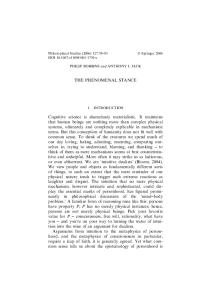
pends on these values alone—an assumption sometimes termed the decision variable assumption (Pelli, 1985). The adoption of this framework allowed us to estimate and compare internal noise for a vast range of tasks, stimuli, and conditions. We found that the value of internal noise is log-normally distributed across this range, and that it is generally higher than reported previously. This high degree of response variability has some interesting implications, which we take up in the Discussion section. Method Origin of Data Sets The data sets used to compute the estimates reported in Figure 1 come from 20 different projects investigating different aspects of sensory processing, all involving a clearly defined signal

d in ′

Sensitivity (d′ Units)

4

2

1

0.5

0.25 0.25

0.5

1

2

4

Internal Noise (Units of External Noise SD) Figure 1. Sensitivity (d′) versus internal noise (abscissa) for a wide range of stimulus conditions and experimental protocols (see the Method section and Table 1 for details). Note: Color is rendered only in the electronic version of this article. Red symbols refer to auditory data sets (1–3); the corresponding red oval is tilted to align with the best-fit line, positioned at center of mass, with parallel-to-line and orthogonal-to-line widths equal to standard deviations of the data across the two axes. For visual data sets (4–20), black symbols refer to static low-level stimuli, magenta to higher level stimuli (Data Sets 14 and 20), blue to moving, green to stereoscopic; corresponding linear-fit ovals are similarly color coded. Symbol size scales with number of forced choice alternatives (2, 4, and 8AFC); square symbols refer to yes–no protocols. Open symbols refer to experiments that are comparable to those performed by Burgess and Colborne (1988). The corresponding oval is shown in gray color, whereas the internal noise range estimated by these authors is indicated by the light-gray shaded rectangular region. The range (6SEM) estimated by Levi et al. (2008) is indicated by the horizontal bar near the x-axis (top); the range estimated by Gold et al. (1999) for high external noise is indicated by the light-magenta shaded rectangular region. Solid vertical and horizontal lines mark unity. Dashed vertical lines mark the range outside which estimates were rejected (see the Method section). Top histogram shows distribution for internal noise with associated Gaussian fit (gray smooth line), right histograms for sensitivity (d ′ immediately next to the axis, d′in [see the Method section for definition] is farther to the right). Arrows indicate mean values. Note that both quantities are plotted to log axes. Colored histograms near the top x-axis plot internal noise distributions (flipped upside-down) for the corresponding subsets (detailed above). Error bars on individual estimates are not shown, to avoid clutter.

804    Neri and a clearly defined external noise source. Both signal and noise were well above visibility/audibility threshold in all experiments. We are not able to qualify this statement more accurately because we did not carry out systematic detection threshold experiments; however, all of the data reported in the present article constituted parts of larger projects that employed noise image classification (Ahumada, 2002) as the main tool. We were able to retrieve clear classification images for all projects, which is a valid indication that external noise was a limiting factor for performance. Doublepass results from less than one third of these projects have been published; however, the focus in these previous publications was not on data from double-pass experiments (which in some cases were not even reported, because they were irrelevant to the general interest of the publication). Table 1 provides a summary of relevant details for each data set. Data sets were treated as separate whenever there were significant differences between the two studies (e.g., although Data Sets 4 and 12 both involved moving dots, stimulus/ target–signal/task were substantially different). In all experiments, the double pass was performed within the same 100-trial block: The last 50 trials were double passes of the first 50 trials in randomly permuted order, and observers were not aware of this manipulation (they did not notice any difference between double-pass and nondouble-pass blocks). Internal Noise Estimation We adopted a procedure similar to the one described by Burgess and Colborne (1988). For an n-AFC task, we assumed that the internal response before the addition of internal noise followed a normal distribution for each of n21 stimuli, and a normal distribution with mean d′in for the stimulus containing the target. Each response was added to a Gaussian noise source with standard deviation σi ; only this noise source differs for repeated presentations and represents internal noise. On each trial, the model selects the stimulus associated with the largest response. Different d′in and σi values correspond to different percentages of correct responses ρ and percentages of same response to repeated presentations α. We selected the two values for d i′n and σi that minimized the mean-square error between the predicted and the observed values for ρ and α. σi estimates outside the 0.2–5 range are not plotted in Figure 1 and were not used for subsequent analysis because they are not robust (see also Burgess & Colborne, 1988); these amounted to ~11% of the whole data set. This relatively high exclusion rate does not necessarily reflect a failure of the methodology per se, since it is at least in part attributable to a lack of sufficient data: The number of trials per estimate collected for excluded estimates (~400 on average) was significantly smaller (at p , .02, unpaired t test) than the number of trials collected for retained estimates (~570). More importantly, this exclusion criterion is not critical to our conclusions, but, if anything, reduces the size of the effect we report for the following reasons: (1) including values outside the 0.2–5 range raises the estimated mean level of internal noise to 1.8; (2) if we restrict analysis to estimates within the bottom 20th percentile for the number of trials and compare it with the top 20th percentile, although we find that (as expected) the latter returns fewer estimates outside the 0.2–5 range, they both return high and similar values for mean internal noise at ~1.7 and ~1.9, respectively. The latter observation indicates that adding more trials per estimate leads to fewer outliers (i.e., it increases the chance of obtaining estimates within a reasonable range), but does not substantially alter the mean estimate over several different attempts. We therefore apply the exclusion criterion detailed previously as a conservative measure: Had we not applied it, our conclusions would have been mostly unchanged or stronger (i.e., higher levels of estimated internal noise). After exclusion, our data set consisted of 419 estimates total. The d′ value plotted on the abscissa in Figure 1 is not d′in but d′, as customarily defined in the literature (Green & Swets, 1966) (i.e., associated with output performance after the addition of internal noise); Figure 1 includes an additional distribution plot (rightmost histogram) for d′in .

Results Figure 1 plots internal noise (in units of external noise, as customary) on the abscissa versus sensitivity (d ′) on the ordinate (Green & Swets, 1966). Sensitivity is narrowly distributed around 1 (0.97  6  0.39 standard deviation [SD]; see arrow near right-hand axis); this is expected, because the stimulus signal-to-noise ratio (SNR) was selected in all experiments so that observers responded correctly on roughly three out of four trials, apart from a limited number of instances in which we explicitly tested SNRs below (½3) and above (23) threshold (see the Discussion section). Internal noise is broadly distributed around 1.3 (1.3560.75 SD) and conforms well to a lognormal distribution (gray fit in upper distribution plot). There was no significant correlation (at p . .05) between d ′ and internal noise, neither across the whole data set ( p 5 .43) or within each of the six subclasses in which we subdivided it in Figure 1 (indicated by different colors and associated oval fits; see the Discussion section for more details). We performed a variety of comparisons across different aspects of this data set. In the present article, we report only those of particular interest. We did not observe significant differences across AFC protocols: Values were 1.360.7 SD (2AFC); 1.260.8 SD (4AFC); 1.460.4 SD (8AFC). Our estimate was lower (at ~0.8) for a series of yes/no experiments (Data Set 13 in Table 1), but this result was related to the specific nature of the stimuli used in those experiments: When we restricted our analysis to 2AFC tasks involving similar stimuli, we obtained an almost identical estimate (see the Discussion section for details and a comparison with previous estimates). Internal noise was significantly higher for auditory (1.760.7 SD) versus visual (1.360.7 SD) experiments (unpaired t test p , .005), despite no significant difference in sensitivity between the two modalities ( p . .05). This difference, however, was not exclusive to intermodality comparisons. We observed, for example, that visual experiments involving stereoscopic stimuli (diamond symbols) returned a higher internal noise estimate (1.961.2 SD) than did those not involving stereoscopic stimulation ( p , .01), and again, this result was not associated with sensitivity differences ( p 5 .6). Discussion The double-pass methodology adopted in the present article was previously used (among others) in Burgess and Colborne (1988). They estimated internal noise for a simple visual detection task. They reported a value of 0.7560.1, almost half of our estimate. Does this mean that our data disagree with theirs? To the contrary, our results are in excellent agreement with those previously reported by these authors. We reach this conclusion by first recognizing that the data sets used in the present study come from wildly different experimental conditions. To provide just one example, some were collected while participants were attempting to detect auditory bursts de-

Mean Number Number of of Trials per Internal No. Stimulus Type Protocol Manipulation Participants Estimate Noise d′in d′ Published Reference   1. Broadband target (A) 2AFC 7 644 1.8 6 0.2 2 6 0.2 1.0 6 0.1   2. Bandpass target (A) 2AFC 6 800 1.7 6 0.2 1.3 6 0.1 0.6 6 0.1   3. Moving target (A) 2AFC 7 938 1.4 6 0.2 1.4 6 0.1 0.8 6 0.1   4. Moving dots 2AFC Temporal modulation 3 1,500 1.7 6 0.5 1.9 6 0.6 1.0 6 0.2 Neri & Levi (2008b)   5. Luminance-defined target 2AFC Surround modulation 6 750 0.8 6 0.1 1.2 6 0.1 0.9 6 0.1 Neri (2009)   6. Texture-defined target 2AFC Surround modulation 6 450 1.0 6 0.1 1.0 6 0.2 0.7 6 0.1 Neri (2009)   7. Stereomotion (dots) 2AFC Adaptation 2 140 1.6 6 0.4 2.7 6 0.7 1.3 6 0.3 Neri & Levi (2008a)   8. Stereo (luminance bars) 2AFC 5 1,193 2.5 6 0.6 1.9 6 0.5 0.7 6 0.1   9. Orientation-defined target 2AFC, 8AFC Attention 4 238 1.0 6 0.1 0.6 6 0.2 0.5 6 0.2 Neri (2004a) 10. Color-defined target 2AFC, 8AFC Attention 4 177 1.4 6 0.2 0.9 6 0.1 0.5 6 0.1 Neri (2004a) 11. Conjunction (orientation 1 color) target 2AFC, 8AFC Attention 4 193 1.1 6 0.1 0.7 6 0.1 0.4 6 0.1 Neri (2004a) 12. Moving dots 2AFC, 4AFC Attention 7 618 1.4 6 0.2 1.7 6 0.1 1.0 6 0.1 13. Luminance bar target Yes–No 6 1,629 0.8 6 0.3 0.8 6 0.1 0.6 6 0.1 14. Natural scenes 2AFC Temporal modulation 8 1,021 1.4 6 0.1 1.7 6 0.1 1.0 6 0.1 15. Moving dots 2AFC Surround modulation 10 255 1.0 6 0.2 1.4 6 0.2 1.0 6 0.1 Neri & Levi (2009) 16. Luminance bar target 2AFC Uncertainty 10 373 1.0 6 0.1 1.4 6 0.1 1.0 6 0.1 Neri (2010) 17. Moving dots 2AFC Adaptation 4 119 1.3 6 0.2 1.7 6 0.2 1.0 6 0.1 18. Orientation-defined target 2AFC Contrast 11 364 1.8 6 0.2 2.4 6 0.2 1.1 6 0.1 19. Moving bar 2AFC Flank modulation 8 850 0.9 6 0.1 1.4 6 0.1 1.1 6 0.1 20. Natural scenes 2AFC Attention 8 313 1.3 6 0.1 1.8 6 0.1 1.0 6 0.1 Note—The description of stimulus type (second column) is followed by (A) to indicate auditory; otherwise, assume visual. Values for internal noise, d in′ (see the Method section for definition) and d ′ are mean 6 SEM. Cells are empty whenever an item is not relevant/available.

Table 1 Itemized Description of the 20 Data Sets Used in This Study

Human Sensory Noise     805

806    Neri livered through headphones, whereas others came from experiments in which they were asked to discriminate local details of natural scenes displayed on a monitor (see Table 1). We do not wish to claim that internal noise is the same across such different conditions, or that it may not depend on other experimental manipulations such as attention, adaptation, and/or task specification. More specifically, in relation to the Burgess and Colborne study, a meaningful comparison requires that we isolate comparable conditions for the experiments included in our data set. We were able to do this for three data sets (5, 13, and part of 16 in Table 1) that involved low-level static luminancedefined targets; the corresponding average estimates for internal noise were 0.83, 0.8, and 0.9 (see light-gray oval in Figure 1). These figures are in excellent agreement with Burgess and Colborne’s overall estimate mostly around 0.8 (see, e.g., their Figure 6) indicated by the light-gray shaded region in Figure 1 (note the overlap with the gray oval). They also agree with the figures reported by Levi and collaborators (Klein & Levi, 2009; Levi, Klein, & Chen, 2008; the corresponding range is indicated by the top horizontal bar in Figure 1). Larger values have occasionally been reported: Green (1964) gave an estimate of 1, and Burgess and Colborne (1988) reported ~1.3 at low SNR. In a more recent study looking at face processing in contrast noise, Gold, Bennett, and Sekuler (1999) reported percent correct and percent agreement values for a 10AFC task (see their Figure 4) corresponding to an internal noise estimate of ~1.1 (high external noise). In order to isolate comparable conditions to those of Gold et al. (1999) from our database, we restricted the analysis to Data Sets 14 and 20 (which involved natural scenes including faces; see Table 1). The corresponding scatter region is indicated by the magenta oval in Figure 1, which overlaps with the range for Gold et al. (1999) detailed above (indicated by light-magenta shaded region in Figure 1). It is tempting to speculate that higher level processing involves more internal noise than does low-level processing, because the overall range spanned by Gold et al.’s (1999) estimates (and our own for natural scenes) seems higher than that associated with low-level stimuli (see previous paragraph). However, we report high internal noise estimates for stereoscopic processing of stimuli that would not customarily be classed as high level (Data Sets 7 and 8; green symbols in Figure 1), indicating that factors besides the low-level/high-level distinction (as understood in the literature) are likely to play a potential role. Notwithstanding the caveats detailed above relating to the role played by specific experimental conditions, we do report that when we plotted our entire population of estimates across all the experimental conditions we tested, its distribution conformed very well to log-normal (Figure 1, top histogram with associated Gaussian fit). It is conceivable that the precise nature of the distribution may differ for different modalities, stimulus types, and other parameters: For example, it is possible that, when restricted to stereoscopic processing, the distribution may not be log-normal. We do not have sufficient data here to

resolve this level of detail; however, the overall result in Figure 1 indicates that, despite potentially measurable differences between individual conditions, at a macroscopic level, the quantity we are examining is likely to be the same: a late source of additive internal noise (this is how we modeled it in order to estimate it in the first place; see the Method section). Because our overall data set is more representative of human sensory processing than is the restricted data set used by Burgess and Colborne (1988), we conclude that if we accept the possibility that a statement such as “human internal noise is in general ~X,” the value for X is 30%–60% larger than is typically assumed in the sensory literature. Our average estimate is slightly smaller (~1.2, range 0.7–1.9) if we compute the mean in log space. As already discussed by Burgess and Colborne (see also Klein & Levi, 2009, and later in the Discussion section), all of the estimates obtained using the methodology exploited in the present article refer primarily to internal noise induced by visible external noise perturbations, which differs from the quantity measured by the equivalent internal noise methodology (Pelli, 1990). What are some of the implications of high internal response variability? Consider, for example, efforts in the literature that fall under the general term molecular psychophysics (Green, 1964; Hirsh & Watson, 1996; Li, Klein, & Levi, 2006; Neri, 2009), whereby the desired goal is to be able to predict not just on what overall percentage of trials the participant responded correctly, but on which exact trials he/she responded correctly or incorrectly. The ability to carry out trial-by-trial prediction is heavily affected by internal noise, because this source of variability is not under direct experimental control: We can attempt to provide a statistical description such as the log-normal distribution in Figure 1, but apart from the external noise applied via the monitor or the headphones, we do not know what configuration internal noise may take on each trial. However, we can ask the following question: Given a certain statistical distribution for internal noise, what is the upper limit on trial-by-trial predictability? In previous work, we have shown that this question can be answered in general terms by establishing a range within which the upper limit for trial-by-trial predictability must lie (Neri, 2009; Neri & Levi, 2006); the exact value within this range depends on the details of the experiment, and it is not possible to determine it without restrictive assumptions, but we can state that it cannot lie outside the specified range in the absence of virtually any assumption at all (Neri & Levi, 2006). More specifically, suppose we run a double-pass experiment and find that a participant gives the same response to repeated presentations on fraction α of the trials (probability of agreement). We can then state that if we are able to construct the best possible model of the participant’s decisional process, our ability to predict the participant’s response may be as low as α or as high as {1 1 √1 1 n[a(n21) 2 1]}/n (for nAFC), depending on the statistical structure of the external stimuli and the internal noise source (Neri & Levi, 2006). The corresponding range for the probability of agreement we measured across our whole data set was 0.7–0.84: This is (on aver-

Human Sensory Noise     807 age) as high as we can expect to be able to predict human responses at threshold in a 2AFC experiment. A second implication is that the efficiency of human sensory processing is expected to sit around 40%. Suppose humans behave like noisy ideal detectors: They process the incoming stimulus ideally, convert it into a decisional variable ideally, add internal noise, and generate a response. By definition, this is as efficiently as they can behave: If their internal noise were 0, their efficiency would be 1. But we know that on average, we expect internal noise to hover around 1.3; this can be easily converted [using ­1/(1 1 x2)] into an efficiency value of ~0.4, with a range between ~0.2 and ~0.7. These values are broadly consistent with those reported in the literature (e.g., Barlow, 1978, 1980; Barlow & Tripathy, 1997; Burgess & Colborne, 1988; Tjan, Braje, Legge, & Kersten, 1995), indicating that the inefficient ideal observer model can often provide a reasonable approximation to the human observer (Cohn & Lasley, 1986). It should be noted, however, that there is extensive evidence documenting inefficiencies not related to internal noise (De Valois & De Valois, 1990); therefore, modeling human observers as noisy ideal detectors may not be appropriate/useful for a number of applications. The suitability of this model (or lack thereof ) must be evaluated on a case-by-case basis, possibly resorting to additional tools beyond standard detectability metrics (see Murray, Bennett, & Sekuler, 2005). A third implication relates to methodologies whose validity depends at least indirectly on the assumed level of internal noise. Consider, for example, certain applications of psychophysical reverse correlation, such as covariance analysis (Neri, 2004b, 2009) or generalized linear modeling (Knoblauch & Maloney, 2008). The former technique partly relies (at least theoretically) on the degree of smoothness of the decisional transducer function (the function that maps the internal decisional variable into a probability of responding correctly or incorrectly) because sharp transducers (e.g., a step function) introduce artifacts within the estimated sensory kernels (Neri, 2004b). If the underlying distribution is smooth and unimodal (as we report in Figure 1), internal noise renders the transducer function smoother, lending support to the analytical treatment that underlies nonlinear kernel estimation using covariance analysis (Neri, 2004b). Internal noise is, however, unwelcome for the application of generalized linear modeling (GLM) to kernel estimation, because Knoblauch and Maloney showed that this approach is ineffective (i.e., no more effective than standard methods; Ahumada, 2002) for internal noise values greater than ~0.5. Less than 5% of our estimates fall below this value, making the GLM approach of very limited utility in realistic applications. All estimates reported in the present article were obtained under the assumption that the underlying process is well captured by a standard signal detection theory model with late additive internal noise source (see the Method section). It is important to be clear about what we mean here by additive: It is simply that noise is added to, rather than multiplying (gain-modulating), the incoming signal. The terms additive and multiplicative have been used by

some authors to refer to different types of internal noise sources, both additive. Additive noise means that the noise intensity does not depend on the intensity of the signal to which the noise is added. Multiplicative noise means that noise intensity scales multiplicatively with the intensity of the signal to which the noise is added (e.g., Klein & Levi, 2009). A significant difficulty with these terms is that there is no general agreement over terminology in the field; indeed, other authors have used other terms, such as contrast-dependent versus contrast-­independent (Gold, Sekuler, & Bennett, 2004). For our purposes, these distinctions are only marginally relevant, in that we estimate the total amount of internal noise that we model as additive in the sense defined above. In line with previous authors (Burgess & Colborne, 1988), we think that this framework is adequate (at least as a macroscopic description of the underlying process within the broad context afforded by our data set) mainly for two reasons. First, as was already noted, the resulting estimates fall within a well-distributed population. Although this result in itself does not validate the adopted methodology, it does suggest that it is a sensible approach for the type of data and application used here. Second, we have demonstrated in previous work that, for a given participant, the estimated amount of internal noise is invariant with respect to the intensity of the target signal over a twofold range (½3 and 23 threshold), despite the large variations in sensitivity and probability of agreement associated with this manipulation (Neri, 2010). A similar result was reported by Gold et al. (1999) and Burgess and Colborne (1988) (although the latter authors also found that in some experimental conditions [see their Figure 4B] internal noise showed a mild [inverse] dependence on SNR). In other words, it appears that internal noise (as estimated using the methodology adopted here) does not depend very much on target intensity, as may be expected of a gain-modulating multiplicative noise source. Instead, it appears to remain constant in units of external noise intensity. Although this result in itself does not validate the SDT framework used to derive it in the first place, it does indicate that the model provides a sensible, robust, and stable description of the underlying mechanism. It is, of course, possible that this final outcome arises from the interaction of multiple different noise sources with different neural characteristics, not necessarily all additive. We are not in a position to address this issue in the present article. Author Note Supported by the Royal Society (University Research Fellowship) and the Medical Research Council (New Investigator Research Grant). I am indebted to Eva Joosten (my collaborator in the auditory experiments) for sharing Data Sets 1–3, Dennis Levi and Stanley Klein for sharing data from Figure 12 in Levi et al. (2008) as well as relevant discussions, Jason Gold for sharing data from Figure 4 in Gold et al. (1999) as well as relevant discussions, and two anonymous reviewers for their comments and criticisms. Correspondence concerning this article should be addressed to P. Neri, Institute of Medical Sciences, University of Aberdeen, Foresterhill, Aberdeen AB25 2ZD, Scotland (e-mail: peter.neri@abdn .ac.uk; [email protected]). Note—Accepted by Cathleen M. Moore’s editorial team.

808    Neri References Ahumada, A. J. (2002). Classification image weights and internal noise level estimation. Journal of Vision, 2(1, Art. 8), 121-131. Barlow, H. B. (1956). Retinal noise and absolute threshold. Journal of the Optical Society of America, 46, 634-639. Barlow, H. B. (1978). The efficiency of detecting changes of density in random dot patterns. Vision Research, 18, 637-650. Barlow, H. B. (1980). The absolute efficiency of perceptual decisions. Philosophical Transactions of the Royal Society B, 290, 71-82. Barlow, H. B., & Tripathy, S. P. (1997). Correspondence noise and signal pooling in the detection of coherent visual motion. Journal of Neuroscience, 17, 7954-7966. Burgess, A. E., & Colborne, B. (1988). Visual signal detection: IV. Observer inconsistency. Journal of the Optical Society of America A, 5, 617-627. Cohn, T. E., & Lasley, D. J. (1986). Visual sensitivity. Annual Review of Psychology, 37, 495-521. De Valois, R. L., & De Valois, K. K. (1990). Spatial vision. Oxford: Oxford University Press. Faisal, A. A., Selen, L. P., & Wolpert, D. M. (2008). Noise in the nervous system. Nature Reviews Neuroscience, 9, 292-303. Gold, J., Bennett, P. J., & Sekuler, A. B. (1999). Signal but not noise changes with perceptual learning. Nature, 402, 176-178. Gold, J., Sekuler, A. B., & Bennett, P. J. (2004). Characterizing perceptual learning with external noise. Cognitive Science, 28, 167207. Green, D. M. (1964). Consistency of auditory detection judgments. Psychological Review, 71, 392-407. Green, D. M., & Swets, J. A. (1966). Signal detection theory and psychophysics. New York: Wiley. Hirsh, I. J., & Watson, C. S. (1996). Auditory psychophysics and perception. Annual Review of Psychology, 47, 461-484. Klein, S. A., & Levi, D. M. (2009). Stochastic model for detection of signals in noise. Journal of the Optical Society of America A, 26, B110-B126. Knoblauch, K., & Maloney, L. T. (2008). Estimating classification images with generalized linear and additive models. Journal of Vision, 8(16, Art. 10), 1-19. Levi, D. M., Klein, S. A., & Chen, I. (2008). What limits performance

in the amblyopic visual system: Seeing signals in noise with an amblyopic brain. Journal of Vision, 8(4, Art. 1), 1-23. Li, R. W., Klein, S. A., & Levi, D. M. (2006). The receptive field and internal noise for position acuity change with feature separation. Journal of Vision, 6(4, Art. 2), 311-321. Murray, R. F., Bennett, P. J., & Sekuler, A. B. (2005). Classification images predict absolute efficiency. Journal of Vision, 5(2, Art. 5), 139-149. Neri, P. (2004a). Attentional effects on sensory tuning for single-feature detection and double-feature conjunction. Vision Research, 44, 30533064. Neri, P. (2004b). Estimation of nonlinear psychophysical kernels. Journal of Vision, 4(2, Art. 2), 82-91. Neri, P. (2009). Nonlinear characterization of a simple process in human vision. Journal of Vision, 9(12, Art. 1), 1-29. Neri, P. (2010). Visual detection under uncertainty operates via an early static, not late dynamic, nonlinearity. Frontiers in Computational Neuroscience, 4, 151. Neri, P., & Levi, D. M. (2006). Receptive versus perceptive fields from the reverse-correlation viewpoint. Vision Research, 46, 2465-2474. Neri, P., & Levi, D. M. (2008a). Evidence for joint encoding of motion and disparity in human visual perception. Journal of Neurophysiology, 100, 3117-3133. Neri, P., & Levi, D. M. (2008b). Temporal dynamics of directional selectivity in human vision. Journal of Vision, 8(1, Art. 22), 1-11. Neri, P., & Levi, D. M. (2009). Surround motion silences signals from same-direction motion. Journal of Neurophysiology, 102, 25942602. Pelli, D. G. (1985). Uncertainty explains many aspects of visual contrast detection and discrimination. Journal of the Optical Society of America A, 2, 1508-1532. Pelli, D. G. (1990). The quantum efficiency of vision. In C. Blakemore (Ed.), Vision: Coding and efficiency (pp. 3-24). New York: Cambridge University Press. Tjan, B. S., Braje, W. L., Legge, G. E., & Kersten, D. (1995). Human efficiency for recognizing 3-D objects in luminance noise. Vision Research, 35, 3053-3069. (Manuscript received March 12, 2010; revision accepted for publication July 17, 2010.)