Hyperspectral Data Compression using a Wiener Filter Predictor Pierre V. Villeneuve, Scott G. Beaven, Alan D. Stocker Space Computer Corporation, 12121 Wilshire Blvd, Suite 910, Los Angeles, CA 90025 ABSTRACT The application of compression to hyperspectral image data is a significant technical challenge. A primary bottleneck in disseminating data products to the tactical user community is the limited communication bandwidth between the airborne sensor and the ground station receiver. This report summarizes the newly-developed “Z-Chrome” algorithm for lossless compression of hyperspectral image data. A Wiener filter prediction framework is used as a basis for modeling new image bands from already-encoded bands. The resulting residual errors are then compressed using available state-of-the-art lossless image compression functions. Compression performance is demonstrated using a large number of test data collected over a wide variety of scene content from six different airborne and spaceborne s ensors.

1. INTRODUCTION Data compression may be described [1] as “the art of finding short descriptions for long strings.” In its simplest form data compression may be thought of as being comprised of two parts: 1.

Model Prediction: whereby new data is modelled using prior data. The information that remains after subtracting the model from the data is then uncorrelated with itself. There does not exist an algorithm for determining the optimal model [2], which makes this task the most challenging part of data compression. This is certainly true so long as we continue to generate larger and more complex data structures.

2.

Entropy Encoder: Higher-frequency data symbols are best described by smaller codes. The optimal code for a given symbol with probability 𝑃𝑖 will have a size of log 2 1⁄ 𝑃𝑖 bits. This task has long been considered a solved problem [3][4], assuming that the residual data is properly decorrelated.

Hyperspectral data [5] is an enabling technology for a great many defense-related applications. A primary bottleneck in disseminating data products to the tactical user community in a timely manner is the limited communication bandwidth between the airborne sensor and the ground station receiver. This report summarizes a new algorithm developed for lossless compression of hyperspectral data. This type of data is highly correlated across spectral bands , and this relationship is exploited by modern target detection algorithms as a means to dramatically mitigate sensitivity to falsealarms originating from scene clutter. The algorithm is named “Z-Chrome” in reference to the ChronoChrome [6] family of change detection algorithms. This algorithm is based on the assumption that compression of spatial information is separable from compression of spectral information. The Z-Chrome algorithm iterates over a sequence of band images from a data cube. At each step a Wiener filter predictor is constructed from the global spectral statistics between the current band and the already -processed data. The model prediction is subtracted from the current band, with the residual band image having spatial content that is now completely decorrelated spectrally from the residual data computed from all other bands. Existing image compression algorithms do a fantastic job at accounting for spatially -correlated image features. Z-Chrome is essentially a spectral-only predictor wrapped around existing state-of-the-art lossless image compression algorithms. Z-Chrome algorithm performance is demonstrated in this report by application to over 700 data cubes collected by six different sensors, including AVIRIS, Hydice, SpecTIR, Hymap, Hyperion and Archer. Quantitative lossless compression performance is measured at the cube level as the average number of bits per pixel. Relative compression performance is reported as the ratio of the compressed file size to the original file size.

2. HYPERSPECTRAL DATA COMPRESSION The philosophy behind this compression effort has been to consider hyperspectral data to be comprised of two independent information domains: spatial and spectral. A number of efforts have attempted to leverage existing multi-dimensional compression tools for application to hyperspectral data. For example, the JPEG-2000 image compression standard has been extended [7] to handle volumetric data from sources such as medical imaging devices . This extension is known as

JPEG 2000, Part 10, or simply JP3D. The JPEG-2000 standard is designed from the beginning to be very flexible and to allow specialized data transforms to be defined for future extensions to different data types. It is natural to consider using this framework for hyperspectral data, as this data is generally stored as a three-dimensional array. Zhang et al. [8] compared two-dimensional (JPEG 2000, Part 2, plus custom spectral KLT [9]) lossless compression with volumetric (JP3D) lossless compression. They note very similar performance for these two methods whe n applied to AVIRIS data from 1997. Another recent effort to leverage existing lossless image tools for hyperspectral data is the “Fast Lossless” compression algorithm developed by the Information Processing Group at the Jet Propulsion Lab in Pasadena, CA [10], [11]. This algorithm is similar in spirit to JPEG-LS [12], [13] lossless image compression in terms of local context modeling. The researchers at JPL extended the scope of the model to also include three samples in the spectral dimension. This algorithm is denoted as JPL-FL in this report and will be discussed in more detail later on. A key aspect to any type of data compression is the phenomenological model used as the basis for making data predictions for comparison with new data. Subtracting the model prediction from new data enables one to decorrelate the sequence of data elements and reduce the overall dimensionality of the data ensemble prior to final entropy encoding. The importance of a well-developed model is demonstrated nicely by Nguyen et al. [14] with regard to more generic sensor data types. The Z-Chrome hyperspectral lossless compression algorithm described in this report is different from most prior efforts in two key aspects: 1.

The distribution of information within a hyperspectral dataset is assumed to be independent and separable from its distribution in the spatial dimension. This enables the use of a spectral-only decorrelation function to operate as a frontend to existing high-quality lossless image compression functions.

2.

Inter-band correlation within hyperspectral data is inherently distributed across all bands [5]. This high degree of correlation enables the construction of a band-to-band prediction scheme that incorporates all spectral information available at any given step. Many prior compression techniques only exploit spectral correlation by building a predictor in a local context with reference to a small number of bands [8], [10], [11], [15].

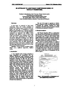
The data flow diagram shown below in Figure 1 illustrates how we view hyperspectral data compression as a chain of three distinct steps: spectral decorrelation, spatial decorrelation, and entropy encoding. All details related to the spectral nature of the data and the Z-Chrome algorithm are fully implemented within the spectral decorrelation module. The output from Z-Chrome is essentially a sequence of single-band residual error images that have been stripped of spectral information correlated with previously processed bands. This residual image may now be processed by any high -quality lossless image compression tool, which in turn must include some form of entropy encoder function. The remainder of this report will focus on the mathematical and implementation details for Z-Chrome and its interface to the remainder of the processing chain.

Figure 1. Hyperspectral data compression chain with separate modules for spectral compression, spatial compression, and entropy encoding. The Z-Chrome algorithm is encapsulated entirely within the spectral decorrelation module on the left side.

3. Z-CHROME ALGORITHM 3.1 Band-Sequential Prediction Model The Z-Chrome compression algorithm is based on statistical signal processing methods commonly used for hyperspectral change target detection. Let 𝑥 𝑖 denote the collection of sensor data for all spatial pixels in band 𝑖. If 𝑥 𝑖 were to be shaped into a two-dimension array it would represent an image of the scene at band index 𝑖. In this discussion the two spatial dimensions are lumped into a single dimension. The entire data cube is represented as a sequence of 𝑁 contiguous bands stacked one atop the other as 𝑋 = [ 𝑏0 , 𝑏1 … , 𝑏𝑁−1 ] 𝑇 . The first- and second-order global statistics of the data are described by a mean vector and a covariance matrix: 𝜇 = 𝐸 [ 𝑋]

(1)

𝐾 = 𝐸 [(𝑋 − 𝜇)(𝑋 − 𝜇) 𝑇 ]

(2)

The task of hyperspectral change detection is described here to provide context for our use of the Wiener filter as a prediction model for data compression. Change detection generally involves two co-registered data cubes acquired at different times over an area where one wishes to determine if any small localized targets have changed between the two times. Assuming the data are each well-described by Gaussian distributions, the change detection problem is optimally addressed by the Wiener filter as implemented by the ChronoChrome algorithm [6], [16], [17]. This procedure amounts to forming a prediction of the second data set from the first, and searching for significant differences in the second data set relative to this prediction. For this scenario, we let 𝑋 denote the first cube, and 𝑌 the second cube. The optimal prediction of 𝑌 from 𝑋 is given by −1 ( 𝑌̂ = 𝐾𝑌 𝐾𝑌𝑋 𝑋 − 𝜇𝑋) + 𝜇𝑌

(3) )𝑇 ]

where 𝐾𝑌 is the covariance matrix of the data 𝑌 and 𝐾𝑌𝑋 = 𝐸[(𝑌 − 𝜇 𝑌 )(𝑋 − 𝜇 𝑋 is the cross-covariance between the two datasets. Change detection is performed by searching for notable differences between 𝑌 and 𝑌̂. The Z-Chrome algorithm uses this very same framework to make predictions of one band of data from the set of already-processed bands. Instead of making predictions across different data cubes as in ChronoChrome, Z-Chrome is instead focused on making predictions across bands within a single data cube. The core unit of work for Z-Chrome is to process the spectral information in a single image band 𝑏𝑘 using as reference the one or more bands of already-processed data 𝑋𝑟𝑒𝑓 = [ 𝑏0 , 𝑏1 , … , 𝑏𝑘−1 ] 𝑇.

(4)

The covariance matrix between the 𝑘 reference bands is computed as a square subset of the full data covariance matrix, 𝐾𝑟𝑒𝑓 = 𝐾 [ 0: 𝑘, 0: 𝑘] .

(5)

The notation 0: 𝑘 indicates the set of band index numbers 𝑖 ∈ ℤ│0 ≤ 𝑖 < 𝑘. The covariance between the set of reference bands and the current working band 𝑘 is given by 𝐾𝑘,𝑟𝑒𝑓 = 𝐾 [ 𝑘, 0: 𝑘] .

(6)

The prediction for the data in band 𝑘 is next given by −1 ( 𝑏̂𝑘 = 𝐾𝑘,𝑟𝑒𝑓 𝐾𝑟𝑒𝑓 𝑋𝑟𝑒𝑓 − 𝜇 𝑟𝑒𝑓 ) + 𝜇 𝑘,

(7)

and the residual that remains after subtracting the prediction from the data in band 𝑘 is 𝜖𝑘 = 𝑏𝑘 − 𝑏̂ 𝑘.

(8)

−1 ( 𝜖𝑘 = ( 𝑏𝑘 − 𝜇 𝑘 ) − 𝐾𝑘,𝑟𝑒𝑓 𝐾𝑟𝑒𝑓 𝑋𝑟𝑒𝑓 − 𝜇 𝑟𝑒𝑓 )

(9)

Substituting from above yields

The residual information 𝜖𝑘 represents the Z-Chrome output product for band 𝑘. The compression and handling of any remaining spatial information is managed by downstream processing elements. These follow-on steps are explained in greater detail in the following sections.

3.2 Z-Chrome Example Prediction Figure 2 below shows an example of what data is involved when performing a single Z-Chrome processing step to real hyperspectral data. In this scenario four bands have already been processed and now serve as reference data (Figure 2, far left) for processing the data in band 𝑘 = 4 (Figure 2, center). The residual error data 𝜖𝑘 (Figure 2, far right) clearly shows that this relatively simple mathematical framework has accounted for a very large fraction of the information contained in the current working band. One can now easily visualize how this grey-scale error image may be passed along downstream to a function that needs only to perform lossless image compression without any knowledge of the hyperspectral nature of the original data. This process is repeated for each band in the dataset. The only exception is that the initial band cannot be processed in this fashion since there does exist reference data with which to make a prediction. In that case only, the band image is passed along directly to the downstream processing stage.

𝑋𝑟𝑒𝑓 = 𝑏0 , … , 𝑏

𝑏𝑘

𝜖𝑘 = 𝑏𝑘 − 𝑏̂𝑘

working band

residual error

𝑇

Figure 2. Example calculation of Z-Chrome band residual with 𝑘 = 4. The stack of four band images of the left is the reference data corresponding to the already -processed image bands. The center image is the current band to be compressed. The image on the right is the result of subtracting the model prediction for band 𝑘 from the current working band.

A

B

Figure 3. Histogram (A) is the distribution of data values contained in the current working band 𝑘 from Figure 2. Histogram (B) is the distribution of data values within the residual error data from the right side of Figure 2.

4. TEST AND EVALUATION FRAMEWORK The dataflow diagram of Figure 1 was implemented in Python software as a flexible framework where different choices for each processing step could be easily evaluated against a large number of test data. This software framework is illustrated below in Figure 4. The two large grey boxes represent the encapsulation of the frontend Z-Chrome functionality as well as the backend lossless image compression functionality. One byproduct of Z-Chrome is a non-negligible amount of metadata, comprised primarily of the scene-average spectrum 𝜇 and covariance matrix 𝐾. The covariance matrix is the second-largest data component to be compressed, after the hyperspectral data itself. In this framework, all metadata is first serialized to compact string representation [18] and then compressed with LZMA (Lempel-Ziv-Markov chain Algorithm) [19] using a fast open-source Python extension [20]. LZMA relies upon dictionary compression plus range encoding. It is a very high-performance lossless compression tool for application to general-purpose data structures. The LZMA function is clearly labelled in Figure 4.

Figure 4. Flexible software framework for evaluating various algorithm choices for the frontend and backend.

The JPEG-LS [7], [12] lossless image compression algorithm serves in this effort as a notional baseline backend compression function. This algorithm is faster than JPEG-2000 and yields considerably better compression than the original lossless JPEG standard [13]. The CharLS [21] C++ library is an open-source implementation of the full JPEGLS standard and was incorporated into this framework by linking it into a C++ Python extension. The local context used by JPEG-LS is shown on the left side of Figure 5, while the local context for JPL’s Fast-Lossless (JPL-FL) algorithm is shown on the right. The JPL hyperspectral algorithm sacrifices one spatial pixel while adding three spectral pixels from previously encoded bands. Initial testing showed that the JPL-FL algorithm results in high a compression ratio while also running very quickly. Of the numerous algorithms discussed in the open literature, it was determined here that JPL-FL would serve as a solid baseline reference method for hyperspectral data compression. A standalone C++ implementation of JPL-FL was developed prior to this current effort as an internal corporate R&D project based on algorithm descriptions from the open literature [10], [11].

Figure 5. Left: Local context models for JPEG-LS lossless image compression JPEG-LS. Right: JPL-FL lossless hyperspectral data compression.

Figure 6. Sample images produced from each of the six sensor types used in this analysis.

5. HYPERSPECTRAL DATA FOR PERFORMANCE TESTING A large number of hyperspectral data cubes were gathered from six different sensor systems to provide a variety of altitudes, noise characteristics, pixel footprints, and size formats. The six sensors include: Hydice [22], Hyperion [23], Hymap [24], AVIRIS [25], ARCHER [26], [27], and SpecTIR [28]. All sensor data used in this study was retrieved from each of the references listed. A top-level overview of the nature of each dataset is shown in Figure 6. In many cases the supplied data was stored in data arrays having a large number of lines. In all cases, data files containing more than 1000 lines were chopped into smaller segments having exactly 1000 lines, with a remainder of arbitrary size less than 1000 lines. The entire dataset is comprised of 735 individual data cubes with a total size of 58.9 GB. All data are stored in individual data files as two-byte unsigned integers.

6. RESULTS Performance analysis was performed by configuring the software test framework of Figure 4 into one of five different modes as indicated in Figure 7. Configuration X corresponds to JPL-FL essentially operating as a standalone application. This mode was managed using the software test framework configured to pass data right through to th e JPL-FL executable. The compression results obtained from JPL-FL will serve as a reference for comparison with compression configurations Y-A through Y-D. The trade study described in this report was designed to shed light onto the nature of how the info rmation contained within hyperspectral datasets may best be compressed given that we quantify information into three categories: Spectral, Spatial, and General. Information spanning the spectral domain might be expected to be well-described with the types of models used by hyperspectral researchers for common tasks such as target detection [29]–[31] and material classification [32]– [34]. Information that primarily spans the spatial domain might instead be expected to be well-handled by methods long used for traditional image compression [35]. Information that spans neither the spectral domain nor the spatial domain might best be handled by a general-purpose compression algorithm such as LZMA [19].

Y-A X Y-B Y-C Y-D Figure 7. Information contained within a hyperspectral data cube is considered here as spanning one or more of the following domains: Spectral, Spatial, and General.

A

B

C

D

Figure 8. Hyperspectral data compression results for 735 data cubes from six different sensors.

The full set of compression results for this report are presented in Figure 8 in the form of compressed bits per band per pixel (or bits/symbol) observed after compressing a given data cube using a particular compression algorithm. These values are easily converted to compression ratio knowing that the original data was stored as unsigned two -byte integers (sixteen bits). This is left as an exercise for the curious reader. Each of the four sub -figures A through D is a scatterplot comparison of a given framework configuration (Y-axis) relative to compression results obtained from the JPL-FL algorithm (X-axis). The color of each data point indicates the sensor type of that particular data cube. The results in the top-left corner, Figure 8-A, show the use of JPEG-LS applied band-by-band on the vertical axis as bits/symbol. The horizontal axis in this same figure shows the compressed bits/symbol obtained from JPL-FL. Recall from earlier that JPL-FL is quite similar in spirit to JPEG-LS, with the exception of sacrificing one pixel of spatial context

in exchange for three pixels of additional spectral context. The use of JPEG-LS on a per band basis is analogous to completely ignoring the correlation of information between any of the bands and instead relying entirely on th e spatial correlation for compression performance. The diagonal line with a slope of 1.0 corresponds to the points where compression performance is identical for both algorithms. In this example, the vast majority of the data points are above the diagonal line, indicating that combined use of spectral and spatial information yields a tremendous improvement in compression performance relative to the use of spatial information alone. The results in the top-right corner, Figure 8-B, show the Z-Chrome frontend combined with a general-purpose LZMA backend. This shows a dramatic change relative to the previous case, Figure 8-A, as now the bulk of the data points fall very close to the diagonal line with a slope of 1.0. The cluster of Archer samples (purple) lies slightly above the line, while the cluster of Hyperion samples (yellow) lies slightly below. It is important to note that this configuration makes no use of spatial correlation and instead relies upon the spectral decorrelation of Z-Chrome to perform the heavy lifting. This is in direct contrast to the previous case (Figure 8-A) where spectral modeling was ignored and spatial modeling was used instead. The results in the bottom-left corner, Figure 8-C, show the Z-Chrome frontend combined with the JPEG-LS backend. This configuration corresponds to the merger of the compression algorithms set up in the two previous results Figure 8-A and Figure 8-B. Comparison of Figure 8-C with Figure 8-B shows a moderate improvement in performance as largely all data points have sunk below the diagonal line with a slope of 1.0. The JPL-FL spatial context model is very similar to the JPEG-LS spatial context model. Thus one possible observation from this result is that the Z-Chrome spectral model leads to improved compression performance over the JPL-FL spectral model. The final result in the bottom-right corner, Figure 8-D, is most similar to the previous case Figure 8-C, except the JPEGLS backend has been replaced by JPL-FL. This particular combination implements spectral compression in both the frontend (Z-Chrome) and in the backend (JPL-FL). This was initially conceived to test if any significant spectral information remained in the residual after Z-Chrome that could be further compressed by JPL-FL. It is not particularly obvious from a qualitative point of view that there is a significant difference between Figure 8-C and Figure 8-D. The most apparent change is the result obtained with the Hyperion data (yellow points). Compression of Hyperion data appears to be slightly better in Figure 8-C. This might be an indication that the slightly better spatial model in JPEG-LS (compared to JPL-FL) is able to take advantage of some particular aspect of the spatial information in this data.

Table 1. Summary quantitative results from the four test scenarios of Figure 8. This table reports on the ratios in compression performance of each test case relative to JPL-FL. The values reported here are as the percentile scores corresponding to 1%, 50% and 99% rank.

A quantitative summary of performance results aggregated over all sensor types is given in Table 1. These values are the result of computing the ratio of each data point’s compressed size relative to that produc ed by JPL-FL. For the ensemble of 735 such ratios, the percentile scores were computed for the percentile ranks of 1%, 50%, and 99%. Ratios above unity indicate performance that is worse than JPL-FL, and are colored orange in the table. Ratios below unity indicate

performance better than JPL-FL, and are colored green in the table. This table of results finally enables us to finish discussing results for the test case shown in Figure 8-D: changing the framework backend from JPEG-LS to JPL-FL yields a rather small improvement on the order of 1%.

7. SUMMARY A software framework was developed with a frontend Z-Chrome component plus a flexible backend component having many choices for compression algorithm. The JPL Fast-Lossless (JPL-FL) algorithm was operated here as a baseline reference for evaluating changes in performance due to the choices made on the selected compression algorithm. The results documented in this report may be summarized by the following observations:  JPEG-LS (i.e. spatial + general) applied to each band independently yields substantially inferior compression performance when compared to other methods that account for spectral correlation  Z-Chrome + LZMA (i.e. spectral + general) yields compression performance only slightly worse than results observed from JPL-FL  Z-Chrome + JPEG-LS (i.e. spectral + spatial + general) yields compression performance slightly better than the results from JPL-FL  Z-Chrome + JPL-FL (i.e. spectral + more spectral + spatial + general) yields very slight improvement beyond those of generated by Z-Chrome + JPEG-LS

8. CONCLUSIONS The results from this analysis provide insight on how one might develop a strategy to efficiently compress hyperspectral image data. It is well known [5], [29] that spectral correlations between data elements in a hyperspectral dataset are significantly stronger than any spatial correlations in the same data. This thought served as the initial motivation for exploring the Z-Chrome band-sequential prediction model. This algorithm operates solely in the spectral domain independently of the spatial domain, and it is this thought that in turn led to the concept of operating Z-Chrome as a preprocessor function operating prior to an already-existing lossless image compression method. The results from this study demonstrate that first- and second-order statistics computed globally may be used to construct a Wiener filter model for band-sequential prediction. The core concept of Z-Chrome is rather straightforward when viewed from a linear algebra perspective, however, this method is unlikely to be considered “low complexity” since each iteration requires direct access to two or more band images. The results presented here clearly indicate that independent handling of spectral versus spatial information is a valid approach for this type of sensor data. In addition to yielding competitive compression performance, this approach also allows for a simpler software architecture that is able to easily leverage existing high -quality spatial compression tools.

9. REFERENCES [1] M. Mahoney, “Data Compression Explained,” 15-May-2013. [Online]. Available: http://mattmahoney.net/dc/dce.html. [2] A. N. Kolmogorov, “Three approaches to the quantitative definition of information,” Probl. Inf. Transm., vol. 1, no. 1, pp. 1–7, 1965. [3] C. E. Shannon, “A Mathematical Theory of Communication,” Bell Syst. Tech. J., vol. 27, pp. 379–423, 623–656, Oct. 1948. [4] S. Verdu, “Fifty years of Shannon theory,” IEEE Trans. Inf. Theory, vol. 44, no. 6, pp. 2057–2078, 1998. [5] M. T. Eismann, Hyperspectral remote sensing, vol. PM210. SPIE PRESS BOOK, 2012. [6] A. Schaum and A. Stocker, “Linear chromodynamics models for hyperspectral target detection,” in 2003 IEEE Aerospace Conference, 2003. Proceedings, 2003, vol. 4, pp. 1879–1885.

[7] “Information Technology - Lossless and near-lossless compression of continuous-tone still images: Extensions,” ITU, Recommendation | International Standard ISO/IEC 14495-2:2003, Mar. 2002. [8] J. Zhang, J. E. Fowler, N. H. Younan, and G. Liu, “Evaluation of JP3D for lossy and lossless compression of hyperspectral imagery,” in Geoscience and Remote Sensing Symposium, 2009 IEEE International, IGARSS 2009 , 2009, vol. 4, pp. IV–474. [9] Q. Du and J. E. Fowler, “Hyperspectral image compression using JPEG2000 and principal component analysis,” Geosci. Remote Sens. Lett. IEEE, vol. 4, no. 2, pp. 201–205, 2007. [10] M. Klimesh, “Low-complexity adaptive lossless compression of hyperspectral imagery,” 2006. [11] N. Aranki, A. Bakhshi, D. Keymeulen, and M. Klimesh, “Fast and adaptive lossless on -board hyperspectral data compression system for space applications,” in Aerospace conference, 2009 IEEE, 2009, pp. 1–8. [12] M. J. Weinberger, G. Seroussi, and G. Sapiro, “The LOCO-I lossless image compression algorithm: principles and standardization into JPEG-LS,” Image Process. IEEE Trans., vol. 9, no. 8, pp. 1309–1324, 2000. [13] S. D. Rane and G. Sapiro, “Evaluation of JPEG-LS, the new lossless and controlled-lossy still image compression standard, for compression of high-resolution elevation data,” Geosci. Remote Sens. IEEE Trans., vol. 39, no. 10, pp. 2298–2306, 2001. [14] Q. Nguyen, H. Jeung, and K. Aberer, “An Evaluation of Model-Based Approaches to Sensor Data Compression,” IEEE Trans. Knowl. Data Eng., 2012. [15] C.-C. Lin and Y.-T. Hwang, “Lossless Compression of Hyperspectral Images Using Adaptive Prediction and Backward Search Schemes,” J Inf Sci Eng, vol. 27, no. 2, pp. 419–435, 2011. [16] A. Schaum and A. Stocker, “Long-interval chronochrome target detection,” in Proc. 1997 International Symposium on Spectral Sensing Research, 1998, pp. 1760–1770. [17] A. Stocker and P. Villeneuve, “Generalized Chromodynamic Detection,” in Geoscience and Remote Sensing Symposium, 2008. IGARSS 2008. IEEE International, 2008, vol. 2, pp. II–609. [18] S. Furuhashi, “Message Pack,” 2013. [Online]. Available: msgpack.org. [19] I. Pavlov, “LZMA Software Development Kit,” 2013. [Online]. Available: 7-zip.org/sdk.html. [20] J. Bauch, “PyLZMA, Python bindings for the LZMA library,” 22-Mar-2011. [Online]. Available: github.com/fancycode/pylzma. [21] Jan de Vaan, “CharLS, a JPEG-LS library,” 09-Nov-2009. [Online]. Available: charls.codeplex.com. [22] “HYDICE Sample Data,” 1995. [Online]. Available: engineering.purdue.edu/~biehl/MultiSpec/hyperspectral.html. [23] “USGS Earth Explorer,” 2013. [Online]. Available: earthexplorer.usgs.gov. [24] “HyMap data sample,” 2013. [Online]. Available: espo.nasa.gov/missions/hs3/image/HyMap_data_sample. [25] M. Eastwood, “AVIRIS Data Locator v2,” 2013. [Online]. Available: http://aviris.jpl.nasa.gov/alt_locator/. [26] “CAP Advanced Technology Group - ARCHER,” 2009. [Online]. Available: members.gocivilairpatrol.co m/emergency_services/operations_support/advanced_technologies.cfm. [27] B. Stevenson, R. O’Connor, W. Kendall, A. Stocker, W. Schaff, R. Holasek, D. Even, D. Alexa, J. Salvador, M . Eismann, R. Mack, P. Kee, S. Harris, B. Karch, and J. Kershenstein, “The civil air patrol ARCHER hyperspectral sensor system,” 2005, vol. 5787, pp. 17–28. [28] “SpecTIR Free Sample Data,” 2012. [Online]. Available: www.spectir.com/free-data-samples/. [29] L. Scharf and C. Demeure, Statistical Signal Processing: Detection, Estimation, and Time Series Analysis, 1st ed. Addison-Wesley, 1991. [30] L. Scharf and B. Friedlander, “Matched Subspace Detectors,” IEEE Trans. Signal Process., 1994. [31] A. P. Schaum, “Spectral subspace matched filtering,” 2001, vol. 4381, pp. 1–17. [32] R. N. Clark, G. A. Swayze, K. E. Livo, R. F. Kokaly, S. J. Sutley, J. B. Dalton, R. R. McDougal, and C. A. Gent, “Imaging spectroscopy: Earth and planetary remote sensing with the USGS Tetracorder and expert systems,” J. Geophys. Res. Planets, vol. 108, no. E12, p. n/a–n/a, 2003. [33] M. E. Winter, “A proof of the N-FINDR algorithm for the automated detection of endmembers in a hyperspectral image,” 2004, vol. 5425, pp. 31–41. [34] A. R. Boisvert, P. V. Villeneuve, and A. D. Stocker, “Endmember finding and spectral unmixing using least -angle regression,” Proc. SPIE, vol. 7695, p. 76951N, 2010. [35] M. Rabbani and R. Joshi, “An overview of the JPEG 2000 still image compression standard,” Signal Process. Image Commun., vol. 17, no. 1, pp. 3–48, Jan. 2002.