Incentives and Efficiency of Pension Systems Maxim Troshkin†
Ali Shourideh
July, 2017 We study the trade-offs between efficiency and incentive costs of social insurance and redistribution when retirement is endogenous. Constrained-efficient pension systems reward later retirement, surprisingly independent of whether efficient retirement ages increase or decrease with productivity. An equivalence result allows us a straightforward characterization of information-constrained efficiency, including a sufficient statistic. We then estimate individual heterogeneity and the parameters of status-quo policies from U.S. income taxes, Social Security, individual earnings, hours, and retirement ages. Unlike in much of optimal taxation literature, optimal retirement policy is capable of generating not only significant welfare gains but also aggregate output gains. JEL codes: E62, H21, H55. Keywords: optimal fiscal policy, social insurance, redistribution, endogenous retirement.
1
Introduction
Motivation. Pension systems are by far the largest component of social insurance in most countries, making their efficiency and the incentives they create a major concern. An optimal system provides productive workers with incentives to fully realize their potential while providing benefits to the individuals experiencing low productivity. On the one hand, standard production efficiency arguments imply that more-productive workers should supply more labor and later retirement could be an aspect of that. On the other hand, one way productive workers are incentivized is with leisure and sufficient needs for incentives could require earlier retirement of more-productive workers. We study these trade-offs and evaluate the constrained efficiency of the U.S. Social Security system, including in incentivizing efficient retirement. We then assess the welfare We thank V.V. Chari, Helmuth Cremer, Mikhail Golosov, Philippe Choné, Roozbeh Hosseini, Mark Huggett, Larry Jones, Nadia Karamcheva, Dirk Krueger, Luigi Pistaferri, Tom Sargent, Nancy Stokey, Aleh Tsyvinski, S¸ evin Yeltekin and numerous seminar and conference participants for valuable input and Tirupam Goel for excellent research assistance. This research was in part supported by the Institute for the Social Sciences. † Shourideh:
[email protected], Carnegie Mellon University, Tepper School of Business. Troshkin:
[email protected], Cornell University, Department of Economics.
1
consequences of optimizing the dynamic nonlinear tax and benefit system, including the optimal dependence of pension benefits on retirement age. This requires a way to qualitatively characterize as well as to quantify constrained efficiency in a realistic model of individual work and retirement choices, with salient features of status quo taxes and benefits and with plausible individual elasticities at both the hours and retirement margins.1 Setup and methodology. We start from a life-cycle framework with individuals ex ante heterogeneous in productivity, which evolves with age, and in fixed costs of working, which are allowed to be correlated with productivity. Fixed costs make individual budget sets non-convex and, combined with hump-shaped productivity-age profiles, make it individually optimal to choose to retire at some age, while choosing a hump-shaped labor supply profile during the working life. The individuals are privately informed about their productivities and their fixed costs. We derive a novel equivalence result giving a straightforward way to characterize information-constrained efficient allocations with endogenous retirement by re-defining the problem in terms of virtual productivities and fixed costs, i.e., accounting for possible information rents. This allows us to establish general properties of a class of income tax and pension systems that implement constrained efficiency but are also close to the U.S. status quo in a way that can be made precise. We then turn to a positive version of the environment, assuming that individuals observed in the U.S. data take the status-quo income taxes and the Social Security as given and make individually optimal choices, which are potentially inefficient. We obtain estimates of the environment parameters using combined micro-level data from the Health and Retirement Survey (HRS) and the U.S. Panel Study of Income Dynamics (PSID). The positive model is able to replicate principle features of reality both internally, in terms of targeted moments such as retirement ages and labor hours, and externally, in terms of the income distribution and the elasticity at the retirement margin. One of the main advantages of our analysis is this ability to reproduce salient features of reality and then, fixing the estimated parameters, to quantify constrained-efficient labor supply, retirement ages, and optimal policies in a coherent framework. We show that this framework extends also to overlapping generations, to accounting for intergenerational transfers, and to heterogeneous life spans. Main qualitative and quantitative findings. First, we qualitatively show that optimal pensions reward later retirement, surprisingly without regard for whether efficient retirement ages increase or decrease with productivity. Intuitively, this is because it is costlier for a planner to provide incentives by distorting retirement ages rather than by distort1 By
retirement we will mean a decision to stop supplying labor. A decision to claim retirement benefits, such as Social Security, will be separate and treated distinctly from the labor force exit decision.
2
ing hours worked. It follows that if optimal retirement distortions are low, in particular lower than hours distortions, pension implementations reward later retirement to counteract the earlier retirement incentives created by income taxes. In other words, optimal pension benefits directly depend on the retirement age so that the present value of lifetime benefits rises with the age of retirement independently of retirement ages increasing or decreasing with productivity. Second, the equivalence result allows us to derive a sufficient statistic for efficient retirement ages to increase or decrease with productivity. Using the sufficient statistic we show that the relationship is driven by individual differences in productivities relative to fixed costs, augmented by the Frisch elasticity of labor supply. It allows us to evaluate how far from efficient the observed retirement ages are by evaluating the sufficient statistic at the retirement ages observed in the data. A quantitatively robust finding is that the efficient retirement ages of individuals with higher lifetime earnings would be higher than in the U.S. data, and also much higher than their less-productive peers. For example, workers in the top half of the lifetime earnings distribution efficiently retire on average at the age of 69.8 in our baseline simulation, while in the U.S. data their average retirement age is 66.9. On the other hand, workers in the bottom half efficiently retire at 61.7, while in the data they do so at 67.6. Third, we quantify how much stronger the incentives for later retirement would need to be from optimal pension systems vs. the existing U.S. Social Security and tax systems. This is achieved by increases in pension benefits in response to delaying retirement. Specifically, efficient marginal pension benefits (with respect to the age of retirement) are positive, quantitatively significant, and increasing with lifetime earnings, e.g., in our baseline from 4.5 percent per year at the bottom of the lifetime earnings distribution to 18 percent at the top.2 Implementing such incentives brings large aggregate welfare gains but, importantly, also aggregate output gains of up to 1.7 percent unlike in much of the optimal taxation literature. Relation to previous findings. Constrained efficiency with extensive margins of labor supply, from various perspectives, is at the center of a related literature with a theoretical focus (e.g., Saez (2002)), which recently showed the optimality of history-dependent distortions when life-cycle considerations are introduced (e.g., Cremer, Lozachmeur, and Pestieau (2004), Michau (2014), Choné and Laroque (2015)). The importance of the contribution of our equivalence result is that – unlike in the previous studies – it enables a straightforward, complete characterization explaining the main forces in terms of stan2 Marginal
pension benefits are well defined in a continuous time setting. Delayed retirement credit in the U.S. Social Security system can be thought of as their analogue in the U.S. data.
3
dard intuitive trade-offs. This facilitates a surprising and completely new to this literature finding – that optimal pension system implementations provide incentives for later retirement independent of whether efficient retirement ages increase or decrease in productivity. Our findings also contribute to a growing empirically-motivated literature bringing theoretical constrained-efficient wedges to estimable distributions and elasticities (e.g., Saez (2001), Golosov, Troshkin, and Tsyvinski (2011), Saez and Stantcheva (2016)). We generalize commonly found tax formulas by connecting standard labor wedges to retirement wedges through estimable elasticities and distributions. An advantage of this connection is the sufficient statistic for the efficient retirement age, a novel finding that is shown to be quite useful. On the quantitative side, most recent studies of optimal redistributive policies largely find that increasing policy distortions (vs. the status quo) significantly improves welfare but generally sacrifices aggregate output, e.g., Weinzierl (2011), Farhi and Werning (2013). In contrast, we show that output may not need to be sacrificed if efficient incentives for retirement are taken into account. Our estimation of the environment parameters uses a mixed identification strategy following recent literature on idiosyncratic consumption and labor choices, e.g., Low, Meghir, and Pistaferri (2010); our use of estimated fixed effects from earnings regressions as types and parts of our exposition follow Low and Pistaferri (2015). We focus on permanent shocks following a literature that finds that most of the welfare gains come not from insurance against temporary shocks but from the provision of social insurance against permanent shocks (e.g., Huggett and Parra (2010)). A related literature finds that permanent shocks similar to the ones we focus on account for most of the variation in lifetime earnings and lifetime utility (e.g., Huggett, Ventura, and Yaron (2011)). Our framework with fixed costs follows recent work applying nonconvex budget sets as a source of retirement decision in life-cycle settings, e.g., Rogerson and Wallenius (2013). An important complementary approach to these general questions is to study policy reforms within a set of parametrically restricted policy instruments as in, e.g., Conesa, Kitao, and Krueger (2009) in the context of dynamic taxation and Huggett and Parra (2010) in the context of Social Security. More recently Golosov et al. (2013) restrict the parametric set to stylized versions of status-quo Social Security and fix taxes, resulting in quite different optima and welfare effects from what we find. Our analysis contributes to that line of research by informing which properties are salient in the choice of the parametric sets of policies. The rest of the paper is organized as follows. Section 2 describes the general envi4
ronment, from both the positive and the normative perspectives. Qualitative properties of the constrained-efficient allocations and optimal policy are characterized in Section 3. Section 4 discusses the construction of a quantitative environment and Section 5 quantifies constrained optima and optimal policies. Section 6 concludes.
2
The Environment
2.1
Normative setup
Consider a continuum of individuals born at t = 0 who live a continuous interval of time ¯ Each individual is born with a type, θ 2 Θ until t = T. θ, θ¯ , drawn at t = 0 from a distribution F (θ ) with F 0 (θ ) = f (θ ) > 0 for all θ. The type affects the idiosyncratic productivity-age profile ϕ (t, θ ): an individual of type θ who chooses at age t to work l (t, θ ) hours produces y (t, θ ) = ϕ (t, θ ) l (t, θ ) units of output. Assume ϕ is twice continuously differentiable and inverse U-shaped, i.e., for each θ 2 Θ there exists an age t such ∂ϕ(t,θ ) ∂ϕ(t,θ ) that ∂t > 0 for all t < t and ∂t < 0 for all t > t . The type also affects the idiosyncratic fixed utility cost of working η (t, θ ): an individual who chooses l (t, θ ) > 0 pays fixed utility cost η (t, θ ) in addition to standard continuous disutility from work. Assume η is continuously differentiable and non-decreasing with age. The preferences of an individual of type θ are given by Z T¯ 0
ρt
e
u (c (t, θ ))
v
y (t, θ ) ϕ (t, θ )
η (t, θ ) 1 fy (t, θ ) > 0g dt,
(1)
where ρ is a subjective discount factor, c (t, θ ) denotes consumption at age t, u is strictly concave, increasing, and satisfies Inada conditions, v is strictly convex with v0 (0) = 0, and 1 f g is an indicator function. The presence of η makes the total disutility of working non-convex, implying non-convex individual budget sets. A non-convex budget set can lead an individual to optimally choose a discontinuous drop in hours at some age, even with continuous hours choice and a preference for smoothing leisure over life.3 An allocation for a cohort of individuals, (c (t, θ ) , y (t, θ ))θ 2Θ,t2[0,T¯ ] , is feasible if Z θ¯ Z T¯ θ
0
e
rt
Z θ¯ Z T¯
c (t, θ ) dtdF (θ ) + H0
θ
3 See,
0
e
rt
y (t, θ ) dtdF (θ ) + rK0 ,
(2)
e.g., Rogerson and Wallenius (2013). They also review empirical evidence that retirement appears as abrupt transitions from full-time work to not working in the U.S. micro data. In the online Appendix C we show similar behavior in a pooled sample of the HRS and the PSID individuals.
5
R T¯ rt where r is the interest rate, H0 Ht dt is the present value of the government 0 e revenue requirement (net outflow of income from the cohort), K0 is initial capital, with both K0 and H0 given. The individuals are privately informed about their productivities and fixed costs. Thus any social insurance cannot contract directly on them but remains otherwise unrestricted, e.g., to be arbitrarily nonlinear or age dependent. To study the problem of a government seeking optimal social insurance, we will characterize the mechanism design problem arising from this information asymmetry. Following standard arguments, the revelation principle guarantees the sufficiency of considering direct mechanisms: individuals report their types to a fictitious planner who chooses allocations subject to incentive compatibility, i.e., for all θ, θˆ 2 Θ Z T¯ 0
e
ρt
u (c (t, θ )) Z T¯ 0
v e
ρt
y (t, θ ) ϕ (t, θ ) "
η (t, θ ) 1 fy (t, θ ) > 0g dt ! # ˆ y t, θ u c t, θˆ v η (t, θ ) 1 y t, θˆ > 0 dt, (3) ϕ (t, θ )
where θ is an individual’s type and θˆ is the individual’s report about the type. The planner’s objective is to maximize a social welfare function Z θ¯
U (θ ) dG (θ ) ,
(4)
θ
where U (θ ) is the lifetime utility of type θ given by (1) and G (θ ) is a cumulative density function, differentiable over θ, θ¯ with G (θ ) = 0, G θ¯ = 1, and G 0 (θ ) = g (θ ) 0. A given exogenous motive to redistribute from higher-earning individuals to lower-earning ones is captured by G (θ ) F (θ ) for all θ 2 θ, θ¯ .4 An allocation is constrained efficient if it is a solution to the direct mechanism design problem of maximizing social welfare (4) subject to incentive compatibility (3) and feasibility (2). Discussion and extensions. This setting is geared toward analyzing implications, particularly welfare implications, of the changes in labor supply at both hours and retirement margins in response to the efficient provision of social insurance. In related environments the welfare gains from labor and capital policies optimized within given sets of functional 4 The
case of G (θ ) = 1 for all θ > θ corresponds to the Rawlsian criterion; G (θ ) = F (θ ) corresponds to the Utilitarian objective. We restrict the differentiability of G to the semi-open interval to include the extremes of redistributive motives like the Rawlsian criterion.
6
forms are extensively studied (e.g., Altig et al. (2001), Conesa, Kitao, and Krueger (2009)). Those gains intuitively come from providing better incentives to save – hence increasing savings – and the resulting effects on the interest rate. Significantly less understanding, however, exists of the labor supply responses, particularly the interaction between the hours and retirement responses. To isolate these mechanisms, we follow recent literature (e.g., Best and Kleven (2013), Farhi and Werning (2013)) in representing the production technology above by an AK-type production function, which is additively separable between labor and capital and therefore allows to abstract from the savings effects.5 While our main discussion will center on a single cohort, an alternative interpretation is the steady state of an overlapping generations economy. We develop an overlapping generations version of this environment in the online Appendix B where each generation is exactly as described above but with additional notation to identify the generations. Another useful extension will be to reinterpret this setting as the problem of a planner attached to one specific generation, i.e., maximizing the welfare of the generation taking as given net intergenerational transfers. We will explore that interpretation in Section 5 where we will think of H0 as the combined present value of government spending and net intergenerational transfers, as well as allowing heterogeneous life span.
2.2
Theoretical wedges vs. policies
Because of the incentive compatibility constraints, efficient allocations could clearly drive wedges into the individual optimality conditions. Before characterizing efficient allocations, it is useful to define the wedges and contrast them with the actual policy tools that can provide implementations. Even though the analysis will extend to the general setup, the following assumption will provide an intuitive benchmark throughout: Assumption 1 For all θ 2 Θ: (i ) η (t, θ ) = η (θ ) otherwise.
∂ ϕθ (t,θ ) ∂t ϕ(t,θ )
0, and (ii ) η (t, θ ) = 0 whenever t < t and
Condition (i ) states that relative productivity differences between types do not diminish with age.6 This is closely related to the observations that the right tail of the income distribution thickens with age and that more-productive individuals tend to have steeper 5 Similarly, parts of that literature also focus on permanent shocks following findings that such shocks account for most of the variation in lifetime earnings and lifetime utility (e.g., Huggett, Ventura, and Yaron (2011)) and that most of the welfare gains come not from redistribution with temporary shocks but from the provision of social insurance against permanent shocks (e.g., Huggett and Parra (2010)). 6 In other words, productivity-age profiles "fan-out". Studies estimating heterogeneous productivity profiles over the life-cycle generally find similar patterns (e.g., Altig et al. (2001), Nishiyama and Smetters (2007)).
7
growth earlier in life and slower decline later in life. This is compatible with most of the population becoming disabled by high enough age. Condition (ii ) is a simple way to assume that participation costs do not diminish with age.7 This ensures that everyone joins the labor force at t = 0, focusing on labor force exit and related policies rather than on the issues related to entering the labor force. Within a positive version of the setup that we discuss below one approach to identifying the fixed costs empirically is from observed individual retirement ages. An identifying assumption in that case is that fixed costs are stable around the observed retirement ages – condition (ii ) will allow us to first develop a simple intuition. We will later relax this assumption and calibrate the rate of change of fixed costs with age to match available estimates of elasticity at the retirement margin. At every age, leisure for each type is affected by individual choices of whether to work and, if so, how much to work; for each type θ there will exist a retirement age – denote it R(θ ) – such that type θ chooses y (t, θ ) > 0 for t < R (θ ) and y (t, θ ) = 0 for t R (θ ).8 We show it formally in the online Appendix A and write allocations as c (t, θ )t2[0,T¯ ] , y (t, θ )t2[0,R(θ )] , R (θ ) . One can then define labor wedge, τ y (t, θ ), and θ 2Θ retirement wedge, τ R (θ ), by the following optimality conditions: 1
(1
τ y (t, θ ) u0 (c (t, θ )) = v0
τ R (θ )) y ( R (θ ) , θ ) u0 (c ( R (θ ) , θ )) = v
y (t, θ ) ϕ (t, θ )
1 , ϕ (t, θ )
y ( R (θ ) , θ ) ϕ ( R (θ ) , θ )
+ η ( R (θ ) , θ ) .
(5)
(6)
Equations (5) and (6) are simply laissez faire individual optimality conditions if both wedges are zero. That is, an efficient allocation that drives a non-zero wedge between the marginal rate of substitution and the marginal rate of transformation distorts the individually optimal consumption-labor choice in (5). Similarly, a wedge in (6) between the marginal utility of income and the marginal disutility of output, which includes the fixed cost, distorts the individual decision about the retirement age R (θ ). The two distortions reflect efficient incentives constrained by the information asymmetry in individual productivities and fixed costs. It is not difficult to see that the wedges of an efficient allocation can have infinitely many actual government policy tools implementing them – a standard property of the 7 It
is sufficient to assume ∂η (θ, t) /∂t 0 throughout. This is easy to see, for example, in the proof of the existence of a retirement age in the online Appendix A. Intuitively, this captures, for example, the deterioration of health with age, making the individuals not only less productive but also increasing their fixed costs of participating in the labor force. 8 See, e.g., Cremer, Lozachmeur, and Pestieau (2004), Choné and Laroque (2015).
8
dynamic mechanism design approach to optimal policy. We propose to focus on a class of policies that not only include implementations of constrained efficiency but also include stylized status quo. Next we define this class in the context of the positive setup, then prove in the next section that the class also contains implementations of efficiency and explicitly characterize their qualitative properties. We later show that with the status-quo policies from this class the positive setup describes reality quantitatively well, allowing the quantitative analysis of efficient policies within a coherent framework.
2.3
Positive setup
Consider a class of government policies consisting of an individual income tax function T and the present value of net retirement benefits b. Taking these policies as given, a type-θ individual maximizes life-time utility (1) subject to the present value budget constraint Z T¯ 0
e
rt
c (t, θ ) dt =
Z R(θ ) 0
e
rt
[y (t, θ )
T (t, y (t, θ ))] dt + b ( R (θ ) , Y (θ )) ,
(7)
where Y (θ ) Y y (t, θ )t2[0,R(θ )] is a measure of lifetime earnings. Note that T is potentially age dependant, but history independent as it is a function of only the current realization of income, while b is a function of the history of incomes. Note also a distinction between the age of claiming benefits and the age of retirement: while per-period benefits depend on both, given an actuarially fair policy the present value of benefits b is a function of the age of retirement.9 Individual optimality conditions can still be written as equations (5) and (6) but with the wedges replaced by the interactions in the policy tools as follows: τ y (t, θ ) = Ty (t, y (t, θ ))
ert δy(t,θ ) Y (θ ) bY ( R (θ ) , Y (θ )) ,
9 That
is, we allow each individual to have access to risk-free savings and borrowing so that the instantaneous budget constraint for a given θ is c (t) + a˙ (t) = 1ft
Rg
(y (t)
T (t, y (t))) + 1ft>Sg b ( R, Y ) e
rS
e ¯
r T¯
/r + ra (t) ,
where a is the level of individual asset holdings and then b ( R, Y ) e rS e r T /r is the per-period benefit claimed starting at age S. Such asset holdings capture, for instance, employer-provided pensions or other tax-deferred accounts.
9
τ R (θ ) y ( R (θ ) , θ ) = T ( R (θ ) , y ( R (θ ) , θ )) e
rR(θ )
erR(θ ) bR ( R (θ ) , Y (θ )) Z T¯
R(θ )
e
rt
dt δ R Y (θ ) bY ( R (θ ) , Y (θ )) ,
where δy(t) Y is the Fréchet derivative of Y with respect to y (t) and δ R Y is with respect to R. Evidently there is a direct connection between the specific properties of the tools in this class of policies and our definitions of the wedges. It gives an intuitive meaning to the wedges. The labor wedge here becomes the balance between the distortions from the marginal income tax and from the marginal benefits with respect to lifetime earnings. The retirement wedge trades off the total tax burden at retirement against the change in benefits coming from adjusting retirement age.
3
Qualitative Properties of Efficient Allocations
To first isolate the forces that are fundamental for the results, we abstract in this section from risk aversion and discounting and set H0 = K0 = 0. For concreteness, assume quasi-linear utility with v (l ) = ψl 1+1/ε / (1 + 1/ε), where ψ is a strictly positive constant and ε 2 (0, ∞) is a Frisch (intensive) elasticity of labor supply. Since the allocation of consumption for an individual is then indeterminate across time, assume without loss of generality that it is constant over the life-cycle, c(θ ). We will relegate formal proofs to the online Appendix A and once we develop the intuition here we will relax these restrictions as well as provide in the online Appendix B formal proofs for the general setup.
3.1
Equivalence result
We start with an equivalence result that will prove notably useful: the mechanism design problem associated with efficient allocations can be characterized by instead considering a simpler "full-information" problem if productivities and fixed costs are re-defined to account for the information rents. Incentive constraints (3) are equivalently a set of lifetime-utility maximization problems, one for each θ, with the choice variable θˆ , a report. Following the first-order approach the incentive compatibility can be written using the envelope theorem as (see, e.g., Kapiˇcka (2013)): 0
U (θ ) =
Z R(θ ) 0
ϕθ (t, θ ) y (t, θ )1+1/ε ψ dt ϕ (t, θ ) ϕ (t, θ )1+1/ε
10
η 0 (θ ) R (θ ) + (η (θ )t (θ ))0 ,
(8)
for all θ 2 Θ, where U (θ ) is the lifetime utility of type θ given by (1). Then the planner’s problem with private information – maximizing welfare (4) subject to feasibility (2) and incentive compatibility (8) with U given by (1) – can be characterized by solving instead the problem omitting incentive compatibility (8) if productivities and fixed costs are appropriately modified:10 Proposition 1 An allocation is constrained efficient if and only if it is efficient with productivity ϕ˜ and fixed costs η˜ given by 1 G (θ ) F (θ ) ϕθ (t, θ ) ϕ˜ (t, θ ) = ϕ (t, θ ) 1 + 1 + ε f (θ ) ϕ (t, θ ) 0 G (θ ) F (θ ) η (θ ) η˜ (θ ) = η (θ ) 1 f (θ ) η (θ )
ε 1+ ε
(9) (10)
What gives rise to this equivalence intuitively is the fact that individuals possess private information about their types and hence a constrained-efficient allocation must allow them to collect rents on that information. Those rents effectively modify productivities and fixed costs to reflect how they are perceived by the individuals. In particular, ϕ (t,θ ) larger relative differences in productivities, ϕθ(t,θ ) , require stronger incentives for more productive types and hence constrained-efficient allocations must deliver larger information rents to those individuals. The modified productivities in (9) capture exactly that, augmented by the Frisch elasticity. Analogous incentives and information-rent effect are η 0 (θ ) produced by larger relative differences in fixed costs, η (θ ) . The modification in (10) accounts for that without the need to account for the hours elasticity. At the same time, G (θ ) F (θ ) stronger preferences for redistribution toward a particular type, , naturally prof (θ ) duce the same effects for both the productivities and fixed costs.
3.2
Sufficient statistic for retirement ages
One immediate benefit of the equivalence result is that it allows one to understand constrainedefficient retirement ages from standard public information trade-offs. Consider a marginal increase in retirement age R (θ ). It has a mechanical effect of increasing output by ϕ˜ ( R, θ ) l ( R, θ ). It also has welfare effects of increasing the disutility of working by 10 We
show in the online Appendix B that with risk aversion the required modification is analogous. To reflect the redistributive motives in G it is no longer enough to compare simply to the distribution of types F since it is no longer the case that social welfare function is the only source of curvature. Hence the comparison there is with a Utilitarian motive accounting for both sources of curvature. One consequence, for instance, is that the modification is no longer degenerate in a Utilitarian case. The modification required by Proposition 1 is also related to the concept of virtual types of Myerson (1981).
11
ψl ( R, θ )1+1/ε / (1 + 1/ε) and by virtual fixed cost η˜ (θ ). At the efficient R (θ ) these effects must balance: output net of variable cost of hours must be equal to the virtual fixed cost. On the other hand, optimality conditions also imply that when hours are chosen efficiently output net of variable cost of hours is proportional to ϕ˜ (t, θ )1+ε . Thus ϕ˜ (t, θ )1+ε /η˜ (θ ) must be equated across types at their efficient retirement ages, i.e., ϕ˜ ( R (θ ) , θ )1+ε /η˜ (θ ) = κ for some constant κ for all θ 2 Θ. Differentiating with respect to θ, the implicit function theorem yields 0
R (θ ) =
∂ ˜ (t, θ )1+ε ∂θ ϕ
/η˜ (θ )
1+ ε
/η˜ (θ )
∂ ˜ (t, θ ) ∂t ϕ
t= R(θ )
.
t= R(θ )
If, for example, individual productivities are declining around retirement, it is efficient to have retirement age increase in θ if and only if ϕ˜ ( R (θ ) , θ )1+ε /η˜ (θ ) increases in θ, and decrease otherwise: Proposition 2 (Sufficient statistic): The constrained-efficient retirement age, R (θ ), increases (decreases) in θ if and only if
1+ ε ∂ ϕ˜ ( R(θ ),θ ) ∂θ η˜ (θ )
0 (
0).
The insight here is that the efficient retirement behavior is driven by how virtual productivities ϕ˜ (t, θ ), augmented by the Frisch elasticity, differ across individuals relative to how different the virtual fixed costs η˜ (θ ) are. While not necessary for the result, Assumption 1 is useful here in focusing on the fundamental forces. It implies that the productivities are increasing in θ at a given age. Since the fixed costs can also be increasing in θ, the resulting retirement behavior must be determined by the relative change. The extent of information asymmetry makes the effective relative change more or less pronounced by adjusting information rents. The equivalence result and hence the sufficient statistic therefore allow us to collapse complex optimality conditions down to a function of a few objects that are relatively straight-forward to interpret.11
3.3
Retirement incentives are costlier than hours incentives
Intuitively, if the retirement wedge is low relative to the labor wedge, the distortion from the income tax provides enough incentives for earlier retirement so that incentives for 11 We show in the online Appendix B that in the general setup with risk aversion and discounting the suf-
ficient statistic is exactly the same. It also does not rely on condition (ii ) in Assumption 1 as ∂η (θ, t) /∂t is sufficient. For an overview of the general approach of sufficient statistics see, e.g., Chetty (2009).
12
0
later retirement must be provided by the pension benefits. If, on the other hand, the retirement wedge is higher than the labor wedge, the distortions from the taxes are not enough to provide efficient incentives for early-enough retirement and it must be also rewarded by the pensions. We show next that under relevant conditions the retirement wedge is smaller than the labor wedge at retirement and that this finding is independent of whether the efficient retirement age pattern is increasing or decreasing. Proposition 3 The wedges implied by the constrained-efficient allocation satisfy τ R (θ ) = τ y ( R (θ ) , θ )
1+
G (θ ) F (θ ) η 0 (θ ) . f (θ ) y ( R (θ ) , θ )
1 ε
In particular, τ R (θ ) < τ y ( R (θ ) , θ ) whenever η 0 (θ )
(11)
0.
This finding is novel and the independence from the retirement age pattern could appear surprising or even counter-intuitive at first. To see the intuition, imagine first a simple example of η 0 (θ ) = 0. Compare the incentive effects of an increase in output via an adjustment in hours vs. an adjustment in the retirement age. A marginal increase in y ( R (θ ) , θ ) by e lowers the utility of working for type θ by an amount proportional to ey ( R (θ ) , θ )1/ε . The same increase in output can be achieved by increasing retirement age R (θ ) by y( R(eθ ),θ ) . This lowers the utility of retiring by an amount proportional to y( R(θ ),θ )1+1/ε 1+1/ε
1/ε
),θ ) = ey( R1+(θ1/ε , which is less than from the adjustment in hours. In other words, when individuals do not differ in fixed costs, the distortions to hours are more useful in providing incentives and consequently the labor wedge at retirement is larger than the retirement wedge. When η 0 (θ ) 0, as will be the case with all of our estimated fixed costs, this mechanism becomes even more pronounced since increasing retirement ages naturally provide additional incentives for the more-productive types not to under-report their type. This is also connected to standard optimal taxation formulas (e.g., the static formulas in Saez (2001) and the dynamic formulas in Golosov, Troshkin, and Tsyvinski (2011)). To show that explicitly, we extend a standard labor wedge formula accounting for the lifecycle with endogenous retirement: for all t and θ 2 Θ, e y( R(θ ),θ )
τ y (t, θ ) = 1 τ y (t, θ )
1+
G (θ ) F (θ ) ϕθ (t, θ ) . f (θ ) ϕ (t, θ )
1 ε
(12)
The difference here is that the labor wedge is scaled up by the relative change in the productivities, ϕθ (t, θ ) /ϕ (t, θ ), reflecting the additional incentives coming from the infor13
mation rents discussed above. Since ϕθ (t, θ ) /ϕ (t, θ ) is increasing in t after the peak productivity t , these incentives provide an additional force beyond standard age-dependence results, increasing the labor wedge with age and making it less costly to keep the retirement distortions lower. In other words, ignoring retirement incentives would lead to optimal policy conclusions that are qualitatively different. Next we show that the main insight here carries through to implementations in the form of optimal pensions rewarding later retirement.
3.4
Optimal pensions reward later retirement
To make policy implementation more intuitive, we explicitly construct the tax and pension benefit functions before showing their qualitative properties. Given constrained, extend y (t, θ ) for t > R (θ ) by definefficient allocation c (θ ) , y (t, θ )t2[0,R(θ )] , R (θ ) θ 2Θ ing it to be the values implied by the virtual productivities (9) if the planner were to ignore the virtual fixed costs (10). This gives a complete profile of income for all ages and individuals. Then the tax function T (t, y) is defined by θ = arg max y t, θˆ θˆ
1+1/ε y t, θˆ ψ . 1 + 1/ε ϕ (t, θ )1+1/ε
T t, y t, θˆ
(13)
Incentive compatibility of (y (t, θ ) T (t, y (t, θ )) , y (t, θ ) , ) pins down the slope of T (t, ) with respect to y. Then over a feasible interval the function T (t, y) is uniquely determined up to a constant: Lemma 1 Given a constrained-efficient allocation with y (t, θ ) continuous and increasing in θ, there exists T (t, y) satisfying (13) that is unique up to a constant on y (t, θ ) , y t, θ¯ . Construct now the benefits b ( R) by first defining bˆ (θ ) = c (θ )
Z R(θ ) 0
[y (t, θ )
T (t, y (t, θ ))] dt.
(14)
Whenever R (θ ) is a one-to-one function of θ, there exists b ( R) such that b ( R (θ )) = bˆ (θ ). If R 6= R (θ ) for some θ, set b ( R) to a sufficiently small number that type θ would never choose. Lemma 2 Given a constrained-efficient allocation with y (t, θ ) continuous and increasing in θ and R (θ ) one-to-one, the policies in (13) and (14) implement the allocation, i.e., the allocation is a local optimum. 14
Intuitively, the tax function T is constructed so that conditional on working in period t an individual of type θ earns exactly the constrained-efficient y (t, θ ). Then the construction of the benefits with formula (14) means that a choice of retirement age R = R θˆ , for ˆ coincides with the choice to report θ. ˆ Given incentive compatibility constraints, some θ, however, the individual of type θ will choose R (θ ). Risk neutrality makes it particularly straightforward to see this intuition because with quasi-linear utility the choice of a retirement age does not affect labor supply at each age. In the general setup with risk aversion a change in the retirement age can affect per-period consumption and hence can change the decision about hours worked at certain ages – it may become individually optimal to double deviate. Nevertheless, we show in the online Appendix B that it is sufficient to condition the benefits function on lifetime earnings to prevent such double deviations. Properties of Optimal Pension Benefits. Assuming differentiable b ( R) (e.g., guaranteed by the differentiability of the allocations) individual optimality conditions imply12 y ( R)
ψ y ( R)1+1/ε T ( R, y ( R)) + b ( R) = + η (θ ) , 1 + 1/ε ϕ ( R)1+1/ε 0
T ( R,y( R))
b0 ( R)
implying that the retirement wedge is given by y( R) and hence from Proposiy( R) tion 3 T ( R, y ( R)) b0 ( R) < Ty ( R, y ( R)) . y ( R) y ( R) That is, pension benefits must reward later retirement, b0 ( R) > 0, whenever marginal tax rates are lower than average tax rates. Even though only the slope Ty (t, y) is uniquely determined at every age, for an arbitrary intercept, the marginal tax is likely to be lower than the average tax at higher incomes. Moreover, since the implementation works for any intercept, T ( , ) can always be modified so that b0 ( R) > 0. A key novel qualitative insight here, just as in the analysis of incentives above, is that pension benefits must reward later retirement independently of whether the efficient retirement ages are increasing or decreasing with productivity: Proposition 4 Given T and b implementing constrained efficiency: (i) Pension benefits reward later retirement whenever average tax is at least as large as marginal tax, i.e., b0 ( R (θ )) > 0 for all θ 2 Θ with T ( R (θ ) , y ( R (θ ) , θ )) /y ( R (θ ) , θ ) Ty ( R (θ ) , y ( R (θ ) , θ )). (ii) There always exist modified Tˆ and bˆ implementing constrained efficiency with the pension benefits rewarding later retirement, i.e., bˆ 0 ( R (θ )) > 0 for all θ 2 Θ. 12 To simplify notation, we suppress here explicit dependence on θ
15
whenever it does not jeopardize clarity.
Properties of Optimal Tax Functions. The explicit construction of T extends to the environment with endogenous retirement the observation that the efficient marginal taxes are generally age dependent. Formula (12) reveals, however, that age dependence is driven also by the properties of the productivity-age profiles. Specifically, whether the efficient marginal tax increases, decreases, or stays unchanged with age will be driven by ϕ (t,θ ) how relative productivity differences evolve with age, i.e., the sign of ∂t∂ ϕθ(t,θ ) . In other words, the rewarding of delayed retirement by optimal pensions is independent of the properties of optimal income tax functions. In particular, that finding is not affected by weather the optimal income taxes are age-dependent or not.13
4
Constructing Quantitative Environment
We now return to the positive version of the setup to estimate parameters of the general environment with risk aversion and discounting using U.S. microeconomic data. We assume each individual in the data takes as given the status-quo income taxes and the U.S. Social Security and maximizes lifetime utility (1) subject to the present-value budget constraint (7) as described in Section 2. The observed individually-optimal allocations are hence potentially constrained inefficient. We use a mixed identification strategy following recent literature on idiosyncratic consumption and labor choices.14 First, some parameters are fixed following existing findings or are taken directly from the observed data. The robustness is checked by changing the values of these parameters within the ranges from the literature and by using alternative definitions in the data. Second, some parameters are estimated outside the environment with ancillary statistical models. For some of these this is done to reduce the computational burden, e.g., for the productivity-age profiles. For others, estimation within the structure of the environment is not needed, e.g., for the status-quo policy functions. In the third step the remaining parameters are calibrated to match data moments, e.g., the unobservable fixed costs. 13 This
can also be seen intuitively more broadly by considering an example with productivity profiles ∂ proportional to each other, i.e., ∂t ϕ (t, θ ) = 0. Then the labor wedge is independent of age and hence so is the marginal tax function (because the marginal rate of substitution between hours worked at different ages is independent of θ and hence all individuals evaluate income at different ages the same way). As a result, variations in the marginal tax across ages cannot be useful in providing incentives. On the other hand, some degree of fanning out in productivity-age profiles can potentially make increasing marginal tax useful for some types after their peak productivity ages t (θ ). 14 See, e.g., Low, Meghir, and Pistaferri (2010).
16
Table 1: Summary statistics for the HRS, the PSID, and the pooled samples. Individuals Observations
HRS sample 971 5,788
PSID sample 1,116 30,751
Pooled sample 2,087 36,539
12.7 (3.1) 0.92 0.87
13.2 (2.5) 0.94 0.84
13.0 (2.8) 0.90 0.88
2272 (635) 35.0 (274.5)
2129 (768) 23.9 (15.8)
2195 (713) 29.1 (187.6)
Years of education Fraction Caucasian Fraction married Average annual hours Average wage
Avg. retirement age, baseline definition 67.4 (5.3) 67.4 (5.3) Avg. retirement age, alternative definition 68.9 (4.8) 64.8 (6.7) 66.7 (6.3) Social Security claiming age 63.5 (2.5) 63.5 (2.5) Notes: 1940-cohort males; standard deviations in parentheses. Sources: RAND HRS, PSID data set from Heathcote, Perri, and Violante (2010).
4.1
Data
Main sources of individual data are the RAND version of the HRS, which is a cleaned and streamlined version of raw HRS files, and the PSID data set from Heathcote, Perri, and Violante (2010), who aim to carefully address a number of well-known issues in the raw data. To take advantage of both the more extensive longitudinal component and the larger retirement age sample, we construct a pooled sample of the HRS and the PSID. The number of individuals from each data set is roughly equal, with the PSID naturally providing significantly more observation per person as summarized in Table 1.15 Summary statistics indicate close sample averages for standard demographic characteristics and hours worked as well as expectedly higher average wage for a more mature HRS sample. Our baseline is the males of the 1940 cohort. One advantage of that cohort is that it is the longest observed cohort in the HRS.16 The bottom three rows of Table 1 also summarize key ages for the setup. We let t = 0 in the model correspond to age 20 and set the baseline life span T¯ = 81.6 following Bell and Miller (2005), extending to heterogeneous life spans T (θ ) later in the next section. The individual ages at which Social Security benefits are claimed, S (θ ), are taken from the HRS. Retirement ages R (θ ) are calculated using two definitions, a baseline and an 15 The
online Appendix C provides further details of the sample construction, the distribution of retirement ages, and how they vary in the data with the definition of retirement, with education, and by sector. 16 Following Guvenen (2009) and Heathcote, Perri, and Violante (2010), we experimented with using all birth years and removing cohort effects with little change to the results below.
17
85 T
80
R
75
R alt
70
S
65 60 1st 2nd 3rd 4th 5th 6th 7th 8th 9th 10th
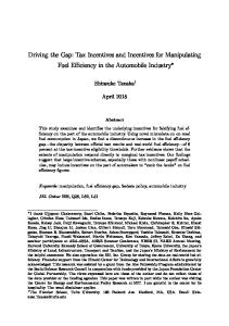
Figure 1: The U.S. microeconomic data (pooled sample of HRS and PSID): retirement ages, R (baseline and alternative definitions), Social Security claiming ages, S, and life expectancy at age 60, T .
alternative. The baseline follows the definition of the consolidated labor force status in the RAND HRS: retirement is recorded when an individual is observed in a non-retired status followed by a permanent switch to the retired status.17 The alternative definition follows Guvenen (2009): retirement is recorded when a worker’s observed annual hours fall below 520 permanently using hours reported in the PSID and the HRS. Figure 1 shows that the retirement ages mildly decrease over much of the lifetime earnings distribution, only slightly increasing over the top two deciles; the Social Security claiming ages are essentially flat to a first approximation around the average of 63.5.
4.2
Productivity-age profiles
The productivity-age profiles are estimated first by adapting a standard parametric approach to our environment (e.g., Altig et al. (2001)). We set ϕ(t, θ ) = θ ϕ(t)θ at , where ϕ (t) is a common component in age, a is a constant, and taking logarithm of both sides, log ϕ (t, θ ) = log θ + log ϕ (t) + at log θ, 17 RAND
HRS reconciles all available relevant responses in each wave. In particular, it aims at separating retirement from unemployment, from partial retirement, and from reporting retirement while also reporting labor earnings.
18
60
0.29
50
0.27
Top 10%
40
0.25
30
0.23
9th decile
20
0.21 5th decile
10 0 20
0.19
1st decile 30
40
50
60
70
at observed R one-year bands five-year bands
0.17 1st 2nd 3rd 4th 5th 6th 7th 8th 9th 10th
80
Figure 2: Idiosyncratic productivity-age profiles estimated on the pooled sample, baseline case, selected percentiles (Panel A). Calibrated fixed costs of working normalized as fractions of time endowment, at the time of observed retirement (baseline R, solid line), one year before and after observed retirement (dot-dashed lines), and five years before and after (dashed lines) (Panel B).
with the first term on the right, log θ, capturing the unobserved idiosyncratic type; the second term, log ϕ (t), is the common age profile; at log θ captures interactions between type and age reflecting that individuals potentially age differently. Following Low and Pistaferri (2015) the individual fixed effects are interpreted as individual type, also helping address potential selection bias. To proxy for log ϕ (t, θ ) the logarithm of effective labor earnings per hour is used, i.e., the computed ratio of all labor earnings to total hours reported, converting to constant 2000 dollars (the year an individual born in 1940 would turn 60).18 We then use predicted individual fixed effects to identify individuals into N types, producing N productivity-age profiles. We focus here on baseline N = 10 with each group representing a lifetime average annual earnings decile and later vary N. Panel A of Figure 2 displays the productivity-age profiles for selected deciles, consistent with the general shape and life-cycle evolution of the profiles in the literature (e.g., Altig et al. (2001)). Higher deciles display higher productivities, generally increasing faster at younger ages. While in this general setup we no longer impose Assumption 1, its condition (i ) is satisfied whenever ϕ (t) decreases at older ages faster than θ at increases. As a result, some fanning out is apparent in productivities with age, at least in the top deciles. 18 The details of the generalized method of moments estimation of the resulting nonlinear statistical model
are reported in the online Appendix C. A significantly more involved alternative is to construct productivities implied by the data and the individual first-order conditions, requiring a structural estimation well outside of the scope of the paper. The main challenge in that case is to correctly account for private assets that appear in the individual optimality conditions with income effects on preferences.
19
As with any parametric procedure, a number of concerns are debated in the literature. To address this, we show that normative findings below are robust with respect to key variations. One potential concern could be data selection: since the time variation can only be identified from the individuals who are still working, it may cause one to overor under-estimate how fast higher productivities decline with age. Following Kahn and Lange (2014), we check robustness to changes in the curvature of the profiles, especially at older ages. We show that the effects of overestimation bias are quantitatively minimal while underestimation works to strengthen our results. Another potential concern could be the sensitivity of the data fit with respect to the parametric assumption about age dependence. To check this robustness we follow Nishiyama and Smetters (2007) grouping individual observations into bins and 10-year intervals of ages, extrapolating by using shape-preserving splines to obtain the complete productivity-age profiles. Then, we also replace age with two alternative definitions of experience to arrive at quantitatively virtually indistinguishable normative insights. The details of these as well as other robustness checks are provided in the online Appendix C.
4.3
Status-quo policies
The policy functions T and b are estimated to match the status-quo U.S. policies. The income tax function is given by
T (y (t)) = y (t)
λy (t)1
τ
.
Functions of this form have been shown to approximate well the effective income taxes in the U.S., inclusive of state income taxes and a number of government non-retirement programs among others (Heathcote, Storesletten, and Violante (2014)). We follow them setting τ = 0.151 (the parameter controlling progressivity) and calibrate λ to equate the present values of lifetime consumption and earnings for the cohort, which is λ = 0.8067 in our baseline. Panel A of Figure 3 shows the resulting marginal and average taxes as functions of annual earnings in constant 2000 dollars. An intuition behind the calibration of λ is easiest to see from the overlapping-generations version of the setup, where the difference between the present values of labor earnings and consumption for a generation is equal to the total net capital income less the present value of government purchases. The net capital income is approximately payments to capital less depreciation, and in standard calibrations in the literature this net capital income as a fraction of GDP would be about 0.4 0.06 3.5 = 0.19, with 0.4 share of capital, 0.06 annual depreciation rate, and the capital-output ratio of 3.5, giving a historical aver20
0.4
$25K $20K
0.2
$15K 0 $10K -0.2 -0.4 $0
$5K
Marginal tax Average tax
Approximation Statutory rate
$0 $50K
$100K
$150K
$0
$50K
$100K
$150K
Figure 3: Estimated U.S. effective personal income tax function, T (Panel A). Approximated U.S. Social Security pension benefit function, B , and annualized PIA benefits as a function of annualized AIME (Panel B). Sources: Heathcote, Storesletten, and Violante (2014), SSA (2014).
age of government purchases around 20% of GDP.19 To estimate the present value of net pension benefits b, we set the annual benefit function to B (Y ) = A 1 + A 2 / 1 + e A 3 Y , where Y is the average value of the highest 35 years of earnings so B (Y ) is the annual R T¯ ¯ 20 Parameters benefit given by b (Y ) B (Y ) S e rt dt, i.e., paid out between S and T. A1 , A2 , and A3 are estimated by minimizing the least absolute deviation of B from the annualized Primary Insurance Amount (PIA) benefit formula of the Old Age, Survivor, and Disability Insurance (OASDI) part of the Social Security in 2000. The benefits are thus a function of a measure of lifetime earnings analogous to the way the PIA is a function of the Average Indexed Monthly Earnings (AIME). Panel B in Figure 3 shows annualized B (Y ) and for comparison PIA, as functions of annual earnings. An advantage of the estimated policies, both the tax and benefit functions, is that they capture key stylized features of the status-quo U.S. policies with relatively simple smooth functions significantly reducing the computational burden. As with the productivity-age profiles, the online Appendix C shows robustness of the normative findings below with respect to alternative estimates of status-quo policies. 19 According the Bureau of Labor Statistics the average value of government consumption expenditure and gross investment as a fraction of GDP between 1947 and 2013 is 20.83. Nevertheless, to explore robustness we also vary this target in the next section. 20 Recall from Figure 1 that in the U.S. micro data individual ages of claiming benefits, S, generally appear quite different from retirement ages, R.
21
4.4
Fixed costs
The fixed costs of working are calibrated within the structure of the positive setup. Preferences are iso-elastic with u (c) =
c1 1
1/σ
1/σ
1
,
v (l ) = ψ
l 1+1/ε , 1 + 1/ε
where ψ is calibrated at the same time as fixed costs to match the average hours in the model to the average hours in the pooled sample. The baseline is σ = 1 with the Frisch elasticity of labor supply ε = 0.5 (mid-range estimates in Chetty (2012)), compared throughout with ε = 0.25. The interest rate is set to 2 percent with β = 0.9804. The fixed costs are calibrated two alternative ways. First, they are simply chosen to match individually-optimal retirement ages in the model to the data. The identifying assumption in this case is that the fixed cost for a given individual type does not change at the ages around retirement, η (t, θ ) = η (θ ) for t in the neighborhood of R (θ ). This is weaker than condition (ii ) in Assumption 1 while still providing an intuitive benchmark. To do this, the positive setup is numerically solved for fixed costs together with allocations, while setting retirement ages, productivity-age profiles, and status-quo policies as described above. The results are shown in Figure 2 for easy comparison with productivities. The solid line in Panel B of Figure 2 plots calibrated fixed costs – at the retirement ages observed in the data – normalized as a fraction of time endowment to facilitate intuition and to allow comparisons with estimates in the literature.21 Average fixed cost in Figure 2 is 0.2306 (e.g., Chang et al. (2014) estimate 0.2099). An interpretation is that on average fixed costs of working represent daily about five and a half hours (23.06 percent of 24 hours) – the time equivalent of commute cost and time, work attire costs, cost of meals, networking, etc. The costs increase with lifetime earnings moderately, from 0.1870 for the bottom earnings decile to 0.2659 at the top of the distribution, consistent with the estimates in the literature.22 Age-varying fixed costs. The second calibration of fixed costs relaxes the restriction of the costs not changing over time in order to capture other forces that may affect retirement, such as variations in health over time. A natural way to calibrate the rate of change from the qualitative analysis that individual optimality requires (1 τ ) ϕt lt u0 (ct ) = v (lt ) + η at ¯ implying yt = ϕ max 0, lt l¯ and the optimality condition t = R. The normalization means a time cost l, t 0 0 ¯ becoming (1 τ ) ϕt u (ct ) = v l at t = R. The time cost l¯ is then equivalent to η if v0 l¯ = v l¯ + η /l¯ ε or l¯ = (η (1 + ε) /ψ) 1+ε . 21 Recall
22 For a review of the estimates in the literature see, e.g., Rogerson and Wallenius (2013). For example, see ¯h in Table 1 in Chang et al. (2014) with γ = 0.5 = 1/ε and the lowest σ x , i.e., closest to permanent shocks (their B = 82.70 is the counterpart of our calibrated ψ = 84.66).
22
in fixed costs with age is to target existing estimates of the elasticity of retirement age with respect to policies affecting retirement decisions. The literature successfully identifying such responses empirically is limited (Chetty et al. (2011)).23 We instead follow French (2005) and use the estimates from his structural life-cycle model of labor supply, health, and retirement. French (2005) reports a range 1.04 - 1.33 of estimates of the elasticity of labor supply with respect to a temporary anticipated increase in earnings at age 60 (see, e.g., his Table 2). He shows that at those ages the individuals are close enough to retirement so that the labor response is coming mainly from the participation decision at the retirement margin. We numerically re-solve the positive setup choosing the rate of change in fixed costs to match the elasticity, while setting fixed costs at the observed retirement ages to the point estimates above since a temporary anticipated increase in earnings leaves unaffected the point-identification. In other words, in the complete calibrated positive setup the fixed costs at the observed retirement ages are pinned down by the individual optimality conditions at those ages while the rate of change of fixed costs with age is calibrated to match the average labor supply elasticity at age 60. The rate of change is calibrated to 1.68% per year targeting the elasticity 1.185, the middle of the range in French (2005). The resulting evolution of fixed costs with age is illustrated also in Panel B of Figure 2. The dot-dashed lines show 1-year bands around the observed retirement ages: fixed costs 1 year before observed retirement ages are shown as a dot-dashed line below the solid line of point estimates; fixed costs 1 year after observed retirement are shown as a dot-dashed line above the point estimates. Similarly, the 5-year bands around the observed retirement ages are shown by the dashed lines. On average, fixed costs 5 years after the retirement ages observed in the data are the equivalent of just over 6 hours per day and by age T the costs exceed 8 hours per day. Given the robustness checks on the productivity-age profiles and status-quo policies above, to be consistent verifying robustness of normative findings in the next section we re-calibrate fixed costs for each of the robustness checks. As a check of external validity of the positive model we also simulate generic extensive labor supply elasticity: starting from the baseline with retirement ages matching the data we compute required simulated change in the present value of lifetime pension benefits to increase the average retirement 23 The robustness of existing estimates is limited primarily by data availability on older individuals’ work-
ing behavior over time, resulting in wide ranges of estimates and challenges singling out the exact elasticity being estimated. A particular challenge is disentangling income and substitution effects. The changes in wages arguably have both income and substitution effects and could be endogenous to health and therefore retirement decision. At the same time, there is limited variation in pension benefits among groups of similar individuals near retirement age.
23
age by one year, giving the average elasticity of 0.37 within the range 0.13 0.43 in the literature (Chetty et al. (2011)). Another standard external validity check is to compare simulated stationary income distribution against an alternative data source. According to the U.S. Census, the median male’s income in the U.S. in 2000 was $37,339 (with a 90% confidence interval of 225.0), while our baseline calibration here is $34,285. The bottom 10 percent of the distribution had average income of $15,722 ( 94.7) vs. calibrated $16,515; the top decile was $85,487 ( 515.1) vs. calibrated $89,905.
5
Quantitative Analysis of Constrained Optima
Given the estimated parameters of the general environment, we return to normative questions to quantify the insights identified by the analysis in Section 3 as well as what they would imply for the overall welfare and aggregate output. Such normative questions ultimately require quantitative answers. One of the main advantages of our analysis is this ability to reproduce salient features of reality and then – fixing the estimated parameters – to quantify constrained-efficient work and retirement behavior and optimal policies in a cohesive framework. Taking advantage of the qualitative insights it is tractable to numerically solve for the constrained-efficient allocations over the complete life-cycle, verify ex post global incentive constraints, and simulate optimal policy implementations. We start with the baseline estimates of productivity-age profiles and fixed costs and with exogenous redistributive motives given by equal weights in the social welfare function, G (θ ) = F (θ ) for all θ 2 Θ. We then vary the welfare weights and the rest of the parameters as described in the previous section to explore quantitative robustness and extensions. Broad quantitative insights that emerge from comparing constrained optima to the status quo are (i ) significantly later retirement of higher earning individuals, (ii ) larger benefits from delayed retirement, which further increase with lifetime earnings, and (iii ) large welfare and output gains from switching to optimal policies.
5.1
Efficient retirement ages
Following our qualitative analysis, we start with the sufficient statistic. Proposition 2 suggests that the profile of constrained-efficient retirement ages across types can be captured in a straightforward way by the differences in virtual productivities relative to fixed costs. Figure 4 illustrates these relative differences as a function of lifetime earnings, evaluated at three sets of ages: at the retirement ages observed in the U.S. microeconomic data, R, 24
18 16 14
at observed S at observed R at age 70
12 10 8 6 1st 2nd 3rd 4th 5th 6th 7th 8th 9th 10th
Figure 4: Sufficient statistic for retirement ages ( ϕ˜ (t, θ )1+ε /η˜ (θ )): evaluated at the retirement ages observed in the U.S. microeconomic data, R (baseline definition), at the Social Security claiming ages, S, and at a constant age 70.
at the observed Social Security PIA-benefit claiming ages, S, and at an arbitrary constant age 70. The sufficient statistic at the observed retirement ages, R, is plotted with a solid line. Given that it is increasing almost everywhere with lifetime earnings, our analysis of Proposition 2 implies that retirement ages should also be increasing almost everywhere to be constrained-efficient, which is in contrast with almost flat profiles we found in Figure 1 for the U.S. data. The sufficient statistic also allows to easily evaluate experiments often put forth as potential goals for pension reforms. Consider hypothetically that, for example, every worker in the U.S. instead is required to retire when they claim their Social Security benefits, i.e. at ages S. Evaluating the sufficient statistic at S for each type produces the dashed line in Figure 4 which is once again increasing for almost all types, suggesting once again that a flat retirement age profile would be suboptimal. Illustrated with the dot-dashed line in Figure 4, the same conclusions are reached if one imagines a hypothetical with every worker retiring instead at a constant age of 70. What experiments like these suggest is that reforms that do not correctly account for the individualized incentives relevant for retirement decisions are likely to keep the economy away from constrained-efficiency. To break down the sources of increasing sufficient statistics recall that we have already seen above in Figure 2 that both the productivities and the fixed costs generally increase with type at a given age. Comparing vertical scales in Panels A and B in Figure 2, it is also apparent that the productivities change much faster with type, in fact close to exponentially, while fixed costs change only about linearly. This is quite intuitive since one expects workers to be potentially vastly more different at productive tasks rather than at
25
A: Retirement ages 85
ε=0.5 ε=0.25 U.S.
0.8 0.6
R
75
B: Retirement distribution 1
0.4
65
0.2 55 1st 2nd 3rd 4th 5th 6th 7th 8th 9th 10th Lifetime earnings deciles
0 55
60
65 70 75 80 Retirement age, R
85
Figure 5: Constrained-efficient retirement ages: As a function of lifetime earnings with Frisch elasticity ε = 0.5 (solid line) and with ε = 0.25 (dashed line) compared to U.S. microeconomic data ( R, baseline definition, dot-dashed line) (Panel A). Cumulative distributions of retirement ages (Panel B).
commute, meals, attire, etc. In terms of virtual productivities and fixed costs, Proposition 1 further implies that information rents only strengthen this relationship (except in the presence of extreme redistributive motives, e.g., Rawlsian motives that we consider below). Turning to the constrained-efficient allocations themselves, Figure 5 illustrates quantitative observations that are robust across variations in the estimated parameters. The solid line in Panel A plots constrained-efficient retirement ages as a function of lifetime earnings in the baseline case with Frisch elasticity ε = 0.5,24 contrasted with the dotdashed line plotting the retirement ages observed in the U.S. micro data (dashed line provides a comparison with ε = 0.25). In line with the sufficient statistic, efficient retirement ages increase for almost all lifetime earnings and strictly increase in the tails of the distribution. The retirement starts from age 57.1 at the bottom of the distribution increasing to 60.1 by the second decile and to 64.5 by median lifetime earnings. The top three deciles show a further increase, bringing the average retirement age for the top half of the distribution to 69.8. The variation in the Frisch intensive elasticity only slightly alters the quantitative extent of these increases. Intuitively, lower intensive elasticity moderately exacerbates individual differences in productivities relative to fixed costs, implying a somewhat steeper sufficient statistic and hence a somewhat steeper retirement age profile. 24 To facilitate comparisons, this baseline case is plotted with a thick solid line throughout the quantitative
analysis as well as later throughout the extensions.
26
The constrained-efficient profiles of retirement ages in Figure 5 are also notably steeper than in the U.S. microeconomic data. The mechanics behind this are that in the bottom half of the distribution the sufficient statistic at the observed retirement ages in Figure 4 is lower than the constrained-efficient value (which would be just below 14), suggesting that those are the ages that are suboptimally high in the data. The opposite holds for the top 20 percent of the distribution (while the 6th through 8th deciles are close to the efficient levels). A comparison of the constrained-efficient solid-line profile with the dot-dashed line of the U.S. retirement ages in Panel A of Figure 5 bears out these observations. Workers in the top half of the lifetime earnings distribution efficiently retire on average at the age of 69.8, while in the U.S. data their average retirement age is 66.9. Workers in the bottom half retire at 61.7, while in the U.S. data they do so at 67.6. For an alternative comparison Panel B also maps these observations into cumulative distributions of retired individuals that are conventional in the literature. Once again the variation in the intensive elasticity minimally alters the quantitative differences.
5.2
Optimal pension systems
Consider next the differences between optimal and the status-quo policies. Another perspective on the sufficient statistic is that the above analysis implies that in the constrained optimum more productive workers need to be provided with incentives for later retirement. A consequence of the sufficient statistic in Figure 4 being above the constrainedefficient values at the top of the lifetime earnings distribution is that the status-quo policy distorts retirement too much in that part of the distribution, resulting in retirement too early. Similarly at the bottom of the distribution the distortion is also too strong (in absolute value) albeit distorting retirement in the opposite direction. Since Proposition 3 shows that retirement incentives are costlier than incentives for the hours decisions, this implies that the status-quo policies cannot be optimal. Wedges. We simulate first the implied wedges in order to illustrate optimal incentives independently of the particulars of an implementation. Panel A in Figure 6 plots the retirement wedge, τ R , as a function of lifetime earnings with a solid line for the baseline ε = 0.5 (as before, the dashed line provides a comparison with ε = 0.25). The positive quantitative framework allows us to also simulate the retirement wedges implied by the U.S. data in the previous section. We plot them as a function of lifetime earnings with a dot-dashed line in Panel A. As explained by the sufficient statistic analysis, for most of the earnings levels and especially in the tails the retirement distortions are reduced in absolute size in the optimum versus the distortions by the status-quo policies. A takeaway 27
B: Labor wedges, ε=0.5
A: Retirement wedges ε=0.25
0.3
0.3
0.2
τ
0
y
0.4
y
0.4
U.S.
R
τ
ε=0.5
τ
0.2
Age 55 Age 40 Age 20
0.1 -0.2
C: Labor wedges, ε=0.25
1 2 3 4 5 6 7 8 9 10 Lifetime earnings deciles
0 1 2 3 4 5 6 7 8 9 Lifetime earnings deciles
0.2 0.1
Age 55 Age 40 Age 20
0 1 2 3 4 5 6 7 8 9 Lifetime earnings deciles
Figure 6: Optimal wedges: Retirement wedge, τ R , with baseline ε = 0.5 and with ε = 0.25 compared with the retirement wedge implied by the status quo U.S. policies (Panel A). Labor wedges, τ y (t), at selected ages with baseline ε = 0.5 (Panel B) compared with ε = 0.25 (Panel C).
is that the existing U.S. policies imply retirement wedges that are significantly more progressive than optimal. That is, quantitatively they distort retirement age decisions in the tails of the earnings distribution too much given how costly the retirement incentives are relative to the hours incentives. The labor wedges, τ y , are shown as functions of lifetime earnings in Panels B and C of Figure 6 for selected ages: at the beginning of the working life (age 20, solid line), at prime (age 40, dashed line), and closer to retirement (age 55, dot-dashed lines). Intuitively, since relative differences between individual productivities tend to increase with age, so do the labor wedges to provide incentives to work at full productivity as explained by our generalization of the standard marginal tax formula (12). The lower Frisch elasticity leads to higher wedges as well. A quantitatively key insight from Figure 6 is that the retirement wedge is of smaller value than the labor wedges everywhere. Recall that our analysis of Propositions 3 and 4 shows that in this case optimal pension systems reward later retirement, regardless of whether the efficient retirement ages are increasing or decreasing. The quantitative differences between the wedges are almost an order of magnitude, implying that sizeable incentives for later retirement are needed to offset the incentives for earlier retirement imbedded in marginal income taxes.25 25 Note
also that while standard results in the literature may suggest to attribute increasing efficient retirement ages to the standard optimality of no distortions for the top type, it cannot be the explanation here. For the top decile, the undistorted labor supply produces a large increase in retirement age from the status quo 68.5 to 81.6, as we have seen in Figure 5. The increases in retirement age, however, are not limited to the top decile. The labor wedge evaluated at retirement for the 9th decile is around 40 percent, yet their retirement age also significantly increases compared with status quo, from 67.2 to 73.6 . Figure 6 reveals that this is due to a significant reduction in their retirement wedge compared with the status quo. Analogous observations hold for the top half of the distribution with the opposite observation for the bottom tail,
28
A: Marginal pension benefit
B: Replacement rate
0.25
3
ε=0.5 ε=0.25 U.S.
0.2 2
0.15 0.1
1
0.05 0 1st 2nd 3rd 4th 5th 6th 7th 8th 9th Lifetime earnings deciles
0 1st 2nd 3rd 4th 5th 6th 7th 8th 9th 10th Lifetime earnings deciles
Figure 7: Optimal pension benefits encourage later retirement (Panel A, marginal benefits with respect to an increase in retirement age). Optimal replacement rates compared to the replacement rates implied by the U.S. microeconomic data and the status-quo U.S. Social Security (Panel B).
Policies. Turning to optimal policy functions, recall from Lemmas 1 and 2 that implementation characterizes marginal policies with the total functions identified up to a constant. To fix the constant (the intercept of the income tax function) we keep the average tax for the bottom decile at -33.3 percent as in the status quo.26 Then the optimal income tax system is fully quantified with the marginal tax rates given by the above analyzed labor wedges in Figure 6. The optimal pension benefits are illustrated in Figure 7. Panel A plots marginal (with respect to an infinitesimal increase in retirement age) pension benefits as a function of lifetime earnings, Bˆ 0 ( R) /Bˆ ( R). The two lines represent the baseline elasticity ε = 0.5 (solid line) and ε = 0.25 (dashed line). Recall that for a type θ facing income taxes T (t, y) and a per-period pension benefit Bˆ ( R) the optimality of the choice of R requires v
y ( R, θ ) ϕ ( R, θ )
+ η (θ ) = u0 (c (θ )) y ( R, θ ) 1
T ( R, y ( R, θ )) y ( R, θ )
Bˆ ( R) 1 + Bˆ 0 ( R) y ( R, θ )
e
r ( T¯ R)
r
!
where intuitively Bˆ 0 ( R) is the rate of return on choosing to retire a bit later so that while the middle of the earnings distribution in the data experience close to optimal retirement incentives as we showed above. 26 According to CBO (2012) the disposable income including transfers of a single parent with one child with an income of $15,000 is approximately $20,000, which amounts to an average tax rate of -33.3 percent. Alternatively, the constant can be fixed, for example, to the rate for the median individual without qualitatively changing the results.
29
Bˆ 0 ( R) /Bˆ ( R) implements the retirement wedge τ R (θ ).27 Panel A shows that the optimal pension system rewards later retirement as explained by the analysis of Proposition 4. The optimal return on later retirement is positive throughout the distribution, ranging from 4.5% at the bottom to 18% at the top of the distribution in the baseline. Optimal marginal benefits increase with earnings, especially in the right tail of the distribution. Intuitively, lower elasticity requires a somewhat steeper profile to provide the same incentives. Our quantitative analysis here also allows a direct comparison with the status-quo U.S. policies. According to SSA (2014), Table 2.A20, the rate of return on later retirement ranged 3.5% 8% between 1987 and 2005. While this is in the same direction as the optimal policy, the quantitative magnitudes are substantially different. Moreover, the status-quo rate of return on later retirement was flat throughout the distribution while it sharply increases in the optimal policy in Panel A of Figure 7. Panel B further quantifies the comparison with the status quo by simulating replacement rates, i.e., the ratio of annual pension benefits to the average annual earnings during the working life, which is a common measure in the literature.28 As before, the solid line plots the baseline ε = 0.5 replacement rates, the dashed line plots replacements rates with ε = 0.25, and the dot-dashed line provides a comparison with the U.S. status-quo replacements rates. The optimal replacement rates decrease as a function of lifetime earnings and in the right tail of the distribution reach levels similar to the status quo. At the bottom of the distribution, relatively earlier constrained-efficient retirement ages and negative average income taxes at retirement require the optimal replacement rate of almost 240 percent compared with just over 100 percent in the status-quo U.S. Social Security system. In other words, as above, the takeaway is a quantitatively significant increase in returns to later retirement.
5.3
Welfare and aggregate output effects
To quantify the importance of the differences illustrated above, we compute the changes in welfare via equivalent consumption variation as well as the changes in output from switching from the U.S. status quo to the baseline simulation of the constrained efficiency. Table 2 compares both the aggregate values and selected percentiles of the lifetime earnings distribution. The top part of Table 2 shows that the aggregate welfare change for the cohort is 7.1% in consumption equivalent. As the analysis above explains, the welfare 27 This illustrates the central mechanism and since the lifetime earnings could also depend on the retirement age the online Appendix B provides the details of computing a complete implementation. 28 Note that the replacement rate is with respect to earnings (not contributions) and will have no effect on the capital stock here. In fact, the pension system does not even have to be pay-as-you-go.
30
Table 2: Effects of switching to baseline optimum from the status quo. Aggregate 7.1%
Changes in Welfare 1st decile 2nd decile 9th decile 44.9% 24.4% -4.7%
10th decile -20.0%
Aggregate 1.7%
1st decile -26.0%
Changes in Output 2nd decile 9th decile -18.7% 1.8%
10th decile 35.0%
in the right tail of the distribution declines – by as much as 20% in the top ten percent of the distribution – while the bottom of the distribution gains significantly – the average of about 12% in the bottom half of the distribution. To understand the sources of large changes in welfare throughout the earnings distribution as well as of the gains in the aggregate, consider how the constrained efficiency affects the output of the economy when the pension system provides individuals with optimal incentives for retirement. The bottom part of Table 2 reveals a substantial growth in aggregate output, increasing it by 1.7 percent. The main driving force behind the increase in aggregate output is the increase in retirement ages we saw in the right tail of the distribution. The combination of reduced retirement wedges we showed above and the persistence of productivity differences with age imply large output gains at the top of the earnings distribution – by more than a third for the most productive decile. Quantitatively, those output gains are more than enough to offset the losses needed for the earlier retirement of the workers in the left tail of the distribution. The resulting significant aggregate output gains contrast with most of the literature, indicative of the potentially underexplored power of retirement incentives as an optimal policy focus.
5.4
Other forces affecting retirement
Next we explore other mechanisms that could reasonably be expected to potentially affect quantitative findings. We focus here on key mechanisms while the online Appendix provides further details of the robustness of the quantitative insights with respect to the alternative definitions of retirement age, alternative estimates of the productivity-age profiles, accounting for alternative measures of experience, varying the steepness of the productivity decline at older ages, alternative status-quo policy approximations, and the number of types. As before, we illustrate the effects focusing on constrained-efficient retirement ages and optimal pension systems to summarize main insights.
31
Heterogeneous life span. Given considerable evidence that mortality is closely related to lifetime earnings (Waldron (2013) among others), we allow for heterogeneous life span in order to explore the effects longer lives could have on efficient retirement and optimal policies by changing the total amount of lifetime benefits collected. This allows us to keep the focus on the efficient retirement ages and optimal pension systems while abstracting from numerous related issues beyond the scope of the paper.29 The environment is as given in Section 2 except the length of life for each individual of type θ is now given by T (θ ) where T : Θ ! R+ is a typically increasing function. The utility function for each individual of type θ is then given by Z T (θ ) 0
e
rt
u (c (t, θ )) dt
Z R(θ ) 0
e
rt
v
y (t, θ ) ϕ (t, θ )
+ η (t, θ ) dt.
(15)
The constrained-efficient allocation is defined as before to be the solution to the mechanism design problem except with preferences given by (15). We re-state the complete modified mechanism design problem in the online Appendix B and formally show that the main channel through which life span can potentially affect the retirement decision is through its income effect on consumption. Thus the quantitative environment can be constructed analogously to Section 4. To obtain the extension of T¯ to T (θ ) we follow Waldron (2013). We use death rates from Chart 1 in Waldron (2013) and apply a standard lifetable calculation. In particular, to extend the death rates beyond the reported age of 71, we calibrate the growth rate in death rate to match the average life expectancy of the cohort to that reported in Bell and Miller (2005) for the 1940 birth year cohort males, given they survived to age 60. The growth rate is calibrated to be 0.37 to match the average cohort life expectancy of 81.6. As a secondary check, we compare the implication for the difference in life expectancy between the lower and the upper halves of the income distribution to those given in Chart 3 in Waldron (2013). For easier comparison earlier in Figure 1 the dot-dashed line plots the average life expectancy for each lifetime earnings decile. Figure 8 plots the resulting efficient retirement ages when life span is heterogeneous (thick dashed line in Panel A) together with the baseline efficient retirement with homogeneous life spans (thick solid line in Panel A). For reference, life expectancy as a function of lifetime earnings is compared with the baseline T¯ in Panel A as well (thin dashed and solid lines respectively). As the analysis in Section 3 suggested, the differences between the efficient retirement ages in the two cases are virtually negligible with the only excep29 One
such aspect of heterogeneous life spans is mortality risk, which adds demand for insurance and makes annuities important. See, e.g., Hosseini and Shourideh (2016), who study the effects of differential mortality on optimal taxes while abstracting from the retirement decision.
32
85 80
0.25 0.2
Life span, T
75 70 65 60
0.15 Retirement age, R 0.1 Homogeneous life span Heterogeneous life span U.S.
0.05
55 1st 2nd 3rd 4th 5th 6th 7th 8th 9th 10th
0 1st 2nd 3rd 4th 5th 6th 7th 8th 9th
Figure 8: The effects of heterogeneity in the life span on efficient retirement ages (Panel A) and on optimal pension design (Panel B).
tion in the top decile of lifetime earnings, who still have to be undistorted but now have a longer life-cycle. This implies that the heterogeneity in life span by itself does not produce large income effects. This however does not mean that the structure of the pension benefits has to stay exactly the same. In fact, the heterogeneity in life span mostly affects the structure of pension benefits and not that of earnings. The quantitative differences in the retirement wedges are still small and hence Panel B illustrates this point with marginal pension benefits. The heterogeneity in life span results in a somewhat flatter profile of marginal pension benefits (dashed vs. solid lines in Panel B), closely resembling to the effects of higher intensive elasticity analyzed above in Figure 7. Intergenerational transfers. A potential limitation is the assumption that the present value of earnings is equal to the present value of consumption for the cohort, assuming away inter-generational transfers through the pension system. An existing pay-as-you-go Social Security system, however, may tend to decrease the present value of consumption relative to that of earnings depending on the replacement rates for a particular generation. Our baseline assumption is not obviously innocuous because intergenerational transfers can affect the labor supply decisions about both the hours worked and the retirement age through income effects. To explore the effects of this argument on our quantitative findings, we next allow for the variations in the difference between the present values of consumption and earnings. Specifically, we modify the calibration of parameter λ in the tax function we described above so that this difference is 10 percent (i.e., net transferring) and also 10 percent (i.e., net receiving) of the present value of earnings. Figure 9 illustrates the resulting changes 33
85 80 75
H/Y=10% H/Y=0% H/Y=-10% U.S.
0.2 0.1 R
70
0
65 60
-0.1
55 50 1st 2nd 3rd 4th 5th 6th 7th 8th 9th 10th
-0.2 1st 2nd 3rd 4th 5th 6th 7th 8th 9th 10th
Figure 9: The effects of intergenerational tranfers on efficient retirement ages (Panel A) and on optimal pension design (Panel B).
to the efficient retirement ages in Panel A and to the optimal retirement wedges in Panel B to summarize the optimal pension system. Expectedly, as the cohort becomes richer in the sense of receiving intergenerational transfers, income effects drive earlier retirement ages. On the other hand, as the cohort transfers part of its earnings the income effects require a steeper retirement age profile. However, these changes do not overturn the overarching insights above about the retirement age profiles. The policy implications are once again similar, with the only noticeable differences in the retirement wedge at the very top of the distribution where it is still optimal to provide incentives to work throughout the life-cycle. Effects of age-varying fixed costs. To quantify the effects of the fixed costs varying with age, we compare the constrained optima using the two alternative calibrations of fixed costs discussed in the previous section. The results are illustrated in Figure 10. Panel A plots the resulting efficient retirement ages with age-varying fixed costs (dashed line) compared with efficient retirement with fixed costs that do not change around the time of retirement (solid line). Similarly, Panel B compares the optimal retirement wedges. To provide a common point of reference, the dot-dashed lines plot the retirement ages observed in the U.S. data (Panel A) and the retirement wedges implied by the data (Panel B). The general insight that more productive individuals retire later than in the U.S. data does not depend on the fixed costs varying with age. Similarly, unlike in the status quo the efficient retirement ages increase over almost all of the lifetime earnings distribution with or without the fixed costs varying with age. While tight identification of fixed costs away from observed retirement behavior is challenging as we discussed in the previous
34
85
75
0.2
Age-varying fixed costs Benchmark fixed costs U.S.
0.1 0 R
80
70
-0.1 -0.2
65
-0.3
60
-0.4
55 1st 2nd 3rd 4th 5th 6th 7th 8th 9th 10th
-0.5 1st 2nd 3rd 4th 5th 6th 7th 8th 9th 10th
Figure 10: The effects of varying fixed costs with age on efficient retirement ages (Panel A) and on optimal pension design (Panel B).
section, this suggests that general insights are quite robust to age-variations. As our analysis in Section 3 explains, there are two competing effects: a mechanical effect of varying costs and an information effect from altered incentives. Start at the bottom of the lifetime earnings distribution where there are no information effects. Compared with stable fixed costs, age-variation lowers costs at the bottom of the distribution since the efficient retirement ages are below the ones observed in the data (the fixed costs in the two cases are the same at the observed retirement ages). Thus mechanically it becomes efficient for the workers at the bottom of the earnings distribution to retire later than if the costs were not varying (the dashed line is above the solid line at the bottom of the distribution in Panel A). This later efficient retirement weakens the incentives of higher-earnings workers to misreport their types, lowering their information rents. Once a worker is high enough in the distribution, however, age-variation increases fixed costs compared with stable fixed costs since the efficient retirement ages are above the ones observed in the data. That creates a trade-off between higher fixed costs and lower information rents: on the one hand, higher fixed costs mechanically require earlier retirement; on the other hand, later retirement lower along the distribution lowers information rents, requiring later retirement. The fact that the dashed line is above the solid line in Panel A in Figure 10 everywhere except at the very top shows that the mechanical cost-variation effects are dominated by the information effects. Consequently retirement ages go up for all but the very top of the distribution. Panel B illustrates this mechanism from the point of view of the optimal pension system. As a result of the above, there is no need for the optimal system to distort retire35
B: Retirement wedges 0
80
-2
70
-4
R
90
τ
R
A: Retirement ages
-6
60
-8 50 1st 2nd 3rd 4th 5th 6th 7th 8th 9th 10th Lifetime earnings deciles
ρ=0 (Rawlsian) ρ=0.5 ρ=1 (Utilitarian)
1st 2nd 3rd 4th 5th 6th 7th 8th 9th 10th Lifetime earnings deciles
Figure 11: The effects of higher redistribution on efficient retirement ages (Panel A) and on optimal pension design (Panel B).
ment age decisions as much and consequently with age-varying fixed costs the retirement wedges are even lower, and everywhere lower than the ones implied by the status quo. Alternative notions of social welfare. To explore the sensitivity of quantitative findings with respect to changing redistributive motives, we set the cumulative social welfare function G (θ ) = F (θ )ρ where ρ 0. The case of ρ = 1 corresponds to the Utilitarian welfare function analyzed in the baseline case above. The cases of 0 ρ < 1 are more redistributive in the usual sense with the extreme of ρ = 0 corresponding to the Rawlsian criterion. The cases of ρ > 1 are the opposite extremes of redistributing away from the bottom of the distribution. Figures 11 and 12 illustrate the effects on retirement ages in Panels A and on the retirement wedges in Panels B. As ρ decreases toward 0, the planner tends to allocate more utility to the left tail of the distribution; in particular, as ρ approaches 0, the left tail of the distribution has to work throughout their life. Intuitively, late retirement prevents moreproductive individuals from pretending to be less productive and decreasing hours while they work, which explains the necessity of large negative wedges in the left tail shown in Panel B of Figure 11. As ρ increases above 1, the level of redistribution toward the left tail declines, producing income effects leading the bottom deciles to retire later; the same redistributive mechanism as above now leads the higher deciles to lower their retirement age except at the very top of the distribution, which has to remain undistorted.
36
A: Retirement ages
70
0.2 0 R
R
80
ρ=1 (Utilitarian) ρ=1.5 ρ=2 (less redistribution)
τ
90
B: Retirement wedges
-0.2
60 50 1st 2nd 3rd 4th 5th 6th 7th 8th 9th 10th Lifetime earnings deciles
-0.4 1st 2nd 3rd 4th 5th 6th 7th 8th 9th 10th Lifetime earnings deciles
Figure 12: The effects of less redistribution on efficient retirement ages (Panel A) and on optimal pension design (Panel B).
6
Conclusions
We analyzed the trade-offs between efficiency and incentive costs of social insurance and redistribution with endogenous retirement. An equivalence result provides a straightforward characterization of the key mechanisms behind constrained optimum and allows us to derive a sufficient statistic for the constrained-efficient retirement ages. Optimal pension systems reward later retirement, surprisingly independent of increasing or decreasing patterns of efficient retirement ages. We found that providing correct individualized work and retirement incentives results not only in significant aggregate welfare gains but also in aggregate output gains. We focused on permanent shocks following the findings that most of the welfare gains come not from redistribution with temporary shocks but from the provision of insurance against permanent shocks (see, e.g., Huggett and Parra (2010)). It suggests that while including temporary shocks may adjust quantitative differences between the status quo and the optimum, the qualitative changes we find would remain.30
References Altig, David, Alan J. Auerbach, Laurence J. Kotlikoff, Kent A. Smetters, and Jan Walliser. 2001. “Simulating Fundamental Tax Reform in the United States.” The American Economic Review 91 (3):574–595. 7, 18, 19 30 An
extension of our framework develops this argument formally in an earlier working paper available upon request.
37
Bell, Felicitie C and Michael L Miller. 2005. “Life Tables for the United States Social Security Area 1900-2100.” Social Security Administration Publication 11 (11536). 17, 32, xx Best, Michael and Henrik Jacobsen Kleven. 2013. “Optimal Income Taxation with Career Effects of Work Effort.” Working Paper . 7 CBO. 2012. “Effective Marginal Tax Rates for Low- and Moderate-Income Workers.” Congressional Budget Office . 29 Chang, Yongsung, Sun-Bin Kim, Kyooho Kwon, and Richard Rogerson. 2014. “Individual and Aggregate Labor Supply in a Heterogeneous Agent Economy with Intensive and Extensive Margins.” Working Paper . 22 Chetty, Raj. 2009. “Sufficient Statistics for Welfare Analysis: A Bridge Between Structural and Reduced-Form Methods.” Annual Review of Economics 1 (1):451–488. 12 ———. 2012. “Bounds on Elasticities with Optimization Frictions: A Synthesis of Micro and Macro Evidence on Labor Supply.” Econometrica 80 (3):969–1018. 22 Chetty, Raj, Adam Guren, Day Manoli, and Andrea Weber. 2011. “Does Indivisible Labor Explain the Difference between Micro and Macro Elasticities? A Meta-Analysis of Extensive Margin Elasticities.” NBER Working Paper No. 16729 . 23, 24 Choné, Philippe and Guy Laroque. 2015. “On the Redistributive Power of Pensions.” Working Paper . 3, 8 Conesa, Juan Carlos, Sagiri Kitao, and Dirk Krueger. 2009. “Taxing capital? Not a bad idea after all!” American Economic Review 99 (1):25–48. 4, 7 Cremer, Helmuth, Jean-Marie Lozachmeur, and Pierre Pestieau. 2004. “Social Security, Retirement Age and Optimal Income Taxation.” Journal of Public Economics 88 (11):2259– 2281. 3, 8 Farhi, Emmanuel and Iván Werning. 2013. “Insurance and Taxation over the Life Cycle.” The Review of Economic Studies 80 (2):596–635. 4, 7 French, Eric. 2005. “The Effects of Health, Wealth, and Wages on Labour Supply and Retirement Behaviour.” Review of Economic Studies 72 (2):395–427. 23 Fudenberg, Drew and Jean Tirole. 1991. Game Theory. MIT Press, Cambridge, Massachusetts. vi
38
Golosov, Mikhail, Ali Shourideh, Maxim Troshkin, and Aleh Tsyvinski. 2013. “Optimal Pension Systems with Simple Instruments.” American Economic Review 103 (3):502–07. 4 Golosov, Mikhail, Maxim Troshkin, and Aleh Tsyvinski. 2011. “Optimal Dynamic Taxes.” NBER Working Paper No. 17642 . 4, 13 Guvenen, Fatih. 2009. “An Empirical Investigation of Labor Income Processes.” Review of Economic Dynamics 12 (1):58–79. 17, 18, xxi Heathcote, Jonathan, Fabrizio Perri, and Giovanni L Violante. 2010. “Unequal We Stand: An Empirical Analysis of Economic Inequality in the United States, 1967–2006.” Review of Economic Dynamics 13 (1):15–51. 17, xviii Heathcote, Jonathan, Kjetil Storesletten, and Giovanni L Violante. 2014. “Optimal Tax Progressivity: An Analytical Framework.” NBER Working Paper No. 19899 . 20, 21 Hosseini, Roozbeh and Ali Shourideh. 2016. “Retirement Financing: An Optimal Reform Approach.” Working Paper . 32 Huggett, Mark and Juan Carlos Parra. 2010. “How Well Does the U.S. Social Insurance System Provide Social Insurance?” Journal of Political Economy 118 (1):76–112. 4, 7, 37 Huggett, Mark, Gustavo Ventura, and Amir Yaron. 2011. “Sources of Lifetime Inequality.” American Economic Review 101 (7):2923–54. 4, 7 Kahn, Lisa B and Fabian Lange. 2014. “Employer Learning, Productivity, and the Earnings Distribution: Evidence from Performance Measures.” The Review of Economic Studies 81 (4):1575–1613. 20 Kapiˇcka, Marek. 2013. “Efficient Allocations in Dynamic Private Information Economies with Persistent Shocks: A First-Order Approach.” The Review of Economic Studies 80 (3 (284)):1027–1054. 10 Low, Hamish, Costas Meghir, and Luigi Pistaferri. 2010. “Wage Risk and Employment Risk over the Life Cycle.” American Economic Review 100 (4):1432–67. 4, 16 Low, Hamish and Luigi Pistaferri. 2015. “Disability Insurance and the Dynamics of the Incentive Insurance Trade-Off.” American Economic Review 105 (10):2986–3029. 4, 19 Michau, Jean-Baptiste. 2014. “Optimal Redistribution: A Life-Cycle Perspective.” Journal of Public Economics 111:1–16. 3 39
Myerson, Roger B. 1981. “Optimal Auction Design.” Mathematics of Operations Research 6 (1):58–73. 11 Nishiyama, Shinichi and Kent Smetters. 2007. “Does Social Security Privatization Produce Efficiency Gains?” The Quarterly Journal of Economics 122 (4):1677–1719. 7, 20, xxiv Rogerson, Richard and Johanna Wallenius. 2013. “Nonconvexities, Retirement, and the Elasticity of Labor Supply.” The American Economic Review 103 (4):1445–1462. 4, 5, 22, xxi Saez, Emmanuel. 2001. “Using Elasticities to Derive Optimal Income Tax Rates.” Review of Economic Studies 68 (1):205–229. 4, 13, viii ———. 2002. “Optimal Income Transfer Programs: Intensive versus Extensive Labor Supply Responses.” The Quarterly Journal of Economics 117 (3):1039–1073. 3 Saez, Emmanuel and Stefanie Stantcheva. 2016. “Generalized Social Marginal Welfare Weights for Optimal Tax Theory.” American Economic Review 106 (1):24–45. 4, viii SSA. 2014. “The Annual Statistical Supplement to the Social Security Bulletin.” Social Security Administration Publication 13 (11700). 21, 30 Waldron, Hilary. 2013. “Mortality Differentials by Lifetime Earnings Decile: Implications for Evaluations of Proposed Social Security Law Changes.” Social Security Bulletin 73 (1):1–37. 32 Weinzierl, Matthew. 2011. “The Surprising Power of Age-Dependent Taxes.” Review of Economic Studies 78 (4):1490–1518. 4
40