Large and Small Firms in a Global Market: David vs. Goliath⇤ Mathieu Parenti† First draft: August 2010. This version: November 2013

Abstract This paper develops a simple model of a “mixed” market structure where monopolistically competitive and oligopolistic firms coexist. The model is characterized by a group of multi-product firms which behave strategically and take their impact on market aggregates into account (e.g. the average price, and total output) and by a monopolistically competitive fringe. Conditions are derived for the coexistence of both types of firms: heterogeneity in production efficiency, captured by economies of scope for large firms, appears as a necessary condition for them to coexist at equilibrium. I then use this model to investigate the impact of globalization on the distribution of the gains from trade. Allowing large firms to have substantial market power affects the distribution of the gains from trade between consumers and producers. I consider free trade as a benchmark and show that it imposes a tougher competitive environment which benefits consumers. On the contrary, when only large firms are able to cover the fixed costs to export, bilateral trade liberalization fosters the exit of small firms, and increases product variety, but it also lowers consumer surplus through a higher average price. Overall, social welfare increases under linear or isoelastic demand but is generally ambiguous.

JEL Classifications: D4, L10, F11 Keywords: Monopolistic Competition, Oligopolistic Market Structure, Large Firms, International Trade. I am very grateful to Lionel Fontagné and Peter Neary for continued guidance. I would also like to thank Claude d’Aspremont, Arnaud Costinot, Mathieu Couttenier, Matthieu Crozet, Ron Davies, Don Davis, Swati Dhingra, Francesco Di Comite, Jonathan Dingle, Gianmarco Ottaviano, Jean Imbs, Sebastien Krautheim, Helene Latzer, Florian Mayneris, Julien Martin, Thierry Mayer, Joan Monras, John Morrow, Volker Nocke, Martin Peitz, Vincent Rebeyrol, Nicholas Schutz, Jacques Thisse, Farid Toubal, Thierry Verdier, Helene Windish and Stephen Yeaple for their helpful comments and suggestions. † CORE - Université Catholique de Louvain, Belgium. E-mail: [email protected]. ⇤

1

1

Introduction

It is well documented that firms are heterogeneous within an industry. For example, exporters are more productive than firms operating on the domestic market only. Heterogeneity in terms of TFP has proved to be robust to many control variables including size, skill, capital intensity, markups and wages (Bernard, Jensen, Redding, and Schott, 2007). Delving further into this heterogeneity, it appears not only that export status matters, but that in most countries, only a small number of firms are responsible for the bulk of exports.1 Following Melitz (2003), the literature has shown how differences in firm productivity may explain such patterns (Redding, 2011). However, the idea that these happy few large, long-lasting firms may behave differently from small firms on the marketplace has hardly been emphasized. The aim of this paper is to tackle the concept of firm heterogeneity from a different perspective. Ruling out differences in productivity, the focus is placed on differences in market behavior and on how these differences matter in the the global economy. To be precise, this paper builds a model of a “mixed” market structure in which a few multiproduct oligopolists and a continuum of single-product monopolistically competitive firms coexist. Two departures are made from the standard models of monopolistic competition. First, the fact that a few large, long-lasting firms drive a major part of aggregate exports suggests that these firms affect the toughness of competition directly. The model thus differs from monopolistic competition by assuming away the Chamberlinian large-group assumption. It features a few large firms behaving strategically while competing with a large number of monopolistically competitive firms. The former take into account how their behavior affects the market outcome, whereas the latter accurately treat market conditions as a given. As emphasized by Baldwin and Gu (2006), Feenstra and Ma (2008), Eckel and Neary (2010), and Ottaviano and Thisse (2010), multi-product firms internalize demand linkages between varieties to determine the breadth of their product scope. The extent to which large firms affect the market outcome depends upon their mass, defined here by the breadth of their product range. At the bottom of the distribution, a large number (formally, 1

Mayer and Ottaviano (2008), Bernard, Jensen, Redding, and Schott (2007) and Manova and Zhang (2009) for respectively Belgium, France, the U.S.A. and China. The same facts hold for trade in services (Crozet, Mirza, and Millet 2010 and Breinlich and Criscuolo 2011).

2

a continuum) of negligible monopolistically competitive firms take the equilibrium average price as given. The second assumption which I relax is the free-entry condition. The monopolistically competitive fringe adjusts to the intensity of competition through entry and exit until profits are driven down to zero. By contrast, to capture the persistence of a few large firms over time, I follow Friedman (1993) for whom free entry is “untenable for oligopolistic markets”. The setting thus features an exogenous number of large firms which earn positive profits in equilibrium.2 Compared to a pure oligopoly setting, the present model takes the importance of the turnover of small firms into account. The main results can be summarized as follows. To develop new insights about the interactions between large and small firms, I consider a closed economy first and show that a firm’s market power increases with its mass. More specifically, large firms charge higher markups than monopolistically competitive firms. This is because large firms are able to manipulate the market aggregate which is relevant to all their competitors’ decisions. Under quadratic preferences and Cournot competition, this aggregate turns out to be the total output. The extent to which large firms are able to manipulate the intensity of competition is captured by the breadth of their product range. Indeed, since consumers exhibit a taste for variety, a greater product range increases a large firm’s share in the total output, and thus its market power. On the contrary, a negligible firm’s only source of market power stems from the characteristics of the product it supplies, which makes this product an imperfect substitute for its competitors’. Second, I take a first step towards understanding the endogenous formation of large firms by deriving conditions for both kinds of firms to coexist in equilibrium. Heterogeneity in productive efficiency emerges endogenously as a necessary condition for a mixed market equilibrium to emerge. In other words, if firms that have the ability to become large do not have an ex-ante cost advantage, they will choose to be negligible in equilibrium. This provides some sound theoretical foundations for assuming ex-ante firm heterogeneity, which is common in the international trade literature where large firms are assumed to have a lower marginal production cost. In my model, heterogeneity in efficiency is captured by the presence of economies of scope for large firms. This condition for the coexistence of large and small firms also puts forward the fact that differences in behavior on the marketplace imply different degrees of 2

Note that these firms are not born big as they choose to be large or not at equilibrium.

3

efficiency. Third, I turn to the case of two open economies and analyze the impact of globalization on the productive structure of each country by investigating the effect of a change in market size and a change in the number of large firms. An increase in market size keeping the number of large firms constant makes the monopolistically competitive fringe more aggressive both through the intensive margin (firms increase their scale, thereby decreasing their average cost) and the extensive margin (new firms enter the market). On the contrary, an increase in the number of large firms raises the average price through the proliferation of new higher-priced varieties. From a domestic producer’s perspective, free trade with an increasing number of countries consists of an increase in market size and the entry of foreign firms on the domestic market. The entry of large foreign firms fosters the exit of small firms but at the same time, the absence of trade frictions makes the potential entry of small firms act as a pro-competitive force. The productive structure in each country is thus affected: the market becomes more concentrated but competition is tougher. The presence of trade frictions (variable and fixed costs) to reach the foreign market alters these predictions significantly. A drop in variable trade costs increases import penetration but in the presence of fixed costs, small firms cannot compensate their domestic losses with their exports to the foreign market, as they can in the free trade scenario. Their scale and markup remain unchanged and the size of the monopolistically competitive fringe shrinks. By contrast, a large firm expands its market share abroad, hence increasing its market power. As a consequence, trade liberalization decreases consumer surplus as the market environment becomes less competitive. Related literature. Our model lies at the intersection of two strands of literature. The first one deals with international trade under oligopoly and the seminal contributions of Dixit and Norman (1980), Brander (1981) and Markusen (1981). In contrast with the industrial organization literature, strategic interactions have not received much attention from trade economists. The lack of robustness in the predictions from early developments of the strategic trade policy literature (Brander and Spencer, 1985; Eaton and Grossman, 1986) is often mentioned as a reason for this lack of interest. In this paper, not only do the results hold whether firms are assumed to compete à la Bertrand instead of à la Cournot, but I show that they hold true for a broad range of preferences. A second reason which Neary (2009) has pointed out to explain the theoretical bias against oligopoly,

4

favoring monopolistic competition is the lack of tractability of the former in general equilibrium (Roberts and Sonnenschein, 1977). However, Neary shows that the problem becomes tractable when considering a market structure in which firms are “large in the small but small in the large,” meaning that each firm impacts competition in its own industry, but not consumer income which is determined at the economy-wide level. Instead, I stick to partial equilibrium here, as the focus is placed on the differences in firms’ market behavior within an industry. The partial equilibrium analysis also allows discussing the distribution of the gains from trade between consumers and producers. When only large firms are able to export, bilateral trade liberalization leads to a monotonic decrease in consumer surplus and a monotonic increase in producer surplus which contrasts with Brander (1981). A second strand of the literature belongs to the industrial organization field. The idea of combining large and small firms within the same setting goes back at least to the dominant firm model developed by Markham (1951). It has also been applied to vertical relationships by Kuhn and Vives (1999) in a setting where large upstream firms trade with small downstream firms. Yet, the coexistence of both types of behavior in a given industry has been neglected. In the conclusion of his celebrated Chamberlinian model of monopolistic competition, Hart (1985) explains the need to invoke oligopoly theory to study a market which “contains a mix of significant and negligible firms.”

To the best of my knowledge, the first paper to deal with competition between big,

strategic firms, and small, monopolistically competitive firms is Shimomura and Thisse (2012). Neary (2010) considers mixed market structures as one of the most promising directions for future research in trade. This is the path taken by the present paper: it is the first paper to address the impact of trade liberalization in a mixed market structure. Besides the motivation for the study of trade liberalization and the endogenous formation of large firms, the closed-economy section of my model also differs from Shimomura and Thisse (2012) in several respects, which will be discussed in Section 2. The remainder of the paper is organized as follows. Section 2 presents the model and determines the conditions under which both large and small firms coexist in equilibrium. Section 3 extends the setting to free trade, while Section 4 determines the effects of trade liberalization for the

5

productive structure of each trading partner. In Section 5, the robustness of the main findings against alternative specifications of preferences is discussed. Section 6 concludes.

2

The Model in a Closed Economy

The economy involves one homogeneous good, produced under perfect competition, one horizontally differentiated good and one factor of production: labor. The supply side of the economy involves a continuum of i 2 [0, M ] negligible (non-atomic) players and ⌦ potentially big firms ! = 1 . . . ⌦ whose mass is N!

0.

With “the mass of a player”, we mean to capture the intuitive idea that heterogeneous firms may impact competition toughness differently in their own industry. This is a source of market power which departs from standard product differentiation. Indeed, the non-atomic players also have some market power (their product is an imperfect substitute for competing varieties), but their price decision alone does not affect their competitive environment. In this sense, such a firm has a zero mass and competes monopolistically. Various reasons may explain why some firms have a stronger impact on competition toughness than others in their industry. The one chosen here is the breadth of the product scope N (!) of firm !, which generalizes the approach taken by Shimomura and Thisse (2012).3 In an industry P with a continuum of varieties of measure V = ⌦ !=1 N (!) + M , the behavior of firm ! affects

market aggregates in its industry directly (e.g. the average price, and total output) as soon as it supplies a positive subset of varieties N! > 0. Note that N (!) 8! 2 [[1, ⌦]] is endogenous and determined by each firm according to a multi-product technology.

2.1

Preferences

On the demand side, there is a continuum of L identical consumers sharing the same preferences. I denote by x!k , xi and X respectively each individual’s consumption of variety k produced by 3

In their framework, big firms are single-product firms with a positive mass. This is hard to reconcile with the idea that a consumer displaying a love for variety smooths its consumption across all varieties. More importantly, the endogenous determination of the product range allows me to discuss the existence of large firms in equilibrium.

6

firm !, of variety i produced by a monopolistically competitive firm, and of all varieties available on the market:

X=

ˆ

x⌫ d⌫ =

V

⌦ ˆ X !=1

N!

x!k dk +

0

ˆ

M

xi di

0

The upper-tier utility function is quasi-linear:

U (A, x) = A + U (x) where x := x⌫V is the consumption mapping of each individual regarding the horizontally differentiated varieties and A is the individual consumption of a homogeneous good produced under pure and perfect competition, used as a numeraire. It is a Hiscksian composite good which absorbs any income effect and places the subsequent analysis in partial equilibrium. The lower-tier utility of consuming the differentiated good is given by a continuum-quadratic utility function: U (x) =

ˆ ✓

↵x⌫

2

V

x2⌫

◆

d⌫

2

✓ˆ

V

x⌫ d⌫

◆2

Each consumer supplies one unit of labor inelastically. She faces the following budget constraint:

A+

ˆ

V

0

p⌫ x⌫ d⌫  R

where R is her income from her wages and a fraction

(1) 1 L

of each firm.4 The parameter ↵

represents the consumer’s intrinsic evaluation of the differentiated good, i.e. its perceived quality: an increase in ↵ shifts expenditure away from the numeraire good towards the differentiated good. Love for variety is captured by . When level X only. Eventually,

= 0, consumers care about the overall consumption

accounts for demand linkages between varieties: the higher

is, the

faster the marginal utility of consuming variety i decreases with the consumption of variety j 6= i. These three parameters are constant across varieties so that at a symmetric consumption path, whether a variety has been produced by a multi-product or single-product firm (respectively MP and SP-firms hereafter) is irrelevant from the consumer’s perspective. 4

This assumption involves no loss of generality. Firms’ ownership does not play any role in this model.

7

Consumption X is split between varieties supplied by SP-firms Xsp and MP-firms Xmp :

X = Xsp + Xmp

Xo :=

⌦ ˆ X

N!

x!k dk

Xm :=

0

1

ˆ

M

xi di

0

First-order conditions for utility maximization with respect to each variety i 2 [0, M ] and each variety k 2 [0, N! ] of firm ! = 1, ..., ⌦ yield the following demand functions 5 : pi = ↵

xi

X

p!k = ↵

x!k

X

The aggregate consumption of a single consumer X appears as a natural proxy for the intensity of competition6 . Given X, the price elasticity increases with the price along the demand curve as in Krugman (1979). The properties of this type of demand matter for comparative statics, but not for cross-sectional analysis: as shown below, the difference in firm behavior itself generates different prices.

2.2

Production

Single-Product Firms SP-firm i faces a downward-sloping demand curve:

p(xi , X) = ↵

xi

X

It takes X as given and maximizes its operating profit (monopolistic competition):

⇡ ⇤m (X) = max(p(xi , X) xi 0

c)Lxi

which leads to the maximizing output as a function of X only: 5 Because utility is linear in the homogenous good, we normalize the marginal utility of income (the Lagrangian) to one. 6 X can be expressed as a function of the average price and the overall mass of varieties V (see Melitz and Ottaviano, 2008).

8

qi⇤ (X) = Lx⇤i (X) = L ·

↵

c 2

X

(2)

8i 2 [0, M ]

⇤ Using symmetry among SP-firms, I drop the subscript i hereafter and note qsp (X) := Lx⇤sp (X)

the output of an SP-firm. Multi-Product Firms Multi-product firms choose their product scope and their output simultaneously in a Cournot-Nash fashion, taking as given the equilibrium total output of other MP-firms and all SP-firms. For the sake of simplicity, I start by analyzing the first-order conditions of MP-firms with respect to the output of each of their varieties and postpone the analysis of the first-order condition with respect to N! to Section 1.4. An MP-firm faces the following demand for each of its varieties:

p(x!k , X) = ↵

x!k

X

When N! > 0, the decisions made by firm ! affect X. It takes as given the equilibrium output X ⇤ ! of all its competitiors:

p!k = ↵

x!k

ˆ

N!

x!k

X

⇤

0

!

where X

⇤

!

=

⌦ ˆ X

! 0 6=!

An MP-firm internalizes that increasing its total output

´ N! 0

0

N! 0

x⇤!0 k dk

+

ˆ

0

M

x⇤i di

x!k decreases the demand for each

of its varieties. Thus, its inverse demand function is steeper than the one faced by an SP-firm. It maximizes its operating profit:

⇧! =

ˆ

N!

(p(x!k , X)

c) Lx!k dk

0

Conditional upon N! , the first-order condition7 with respect to x!k leads to the profit-maximizing 7

Strictly speaking, the firm maximizes a functional with respect to an output profile. This optimization problem can be solved using calculus of variations in the spirit of Baldwin and Ottaviano (1998): consider the variation "⌘(k) with " > 0 and ⌘(k) an arbitrary continuous function satisfying ⌘(0) = ⌘(N! ) = 0. Taking the derivative

9

quantity of each variety:

↵

c

2

x⇤!k

2

ˆ

N!

0

x⇤!k dk

(3)

X⇤ ! = 0

so the density of output of firm ! is uniform across its varieties and can be expressed as a function of X only:

x⇤!k (X) = x⇤! (X) =

↵ c X 2 + N!

Notice that x! = xm when N! = 0. I now turn to the relationship between a firm’s “mass” and its pricing behavior.

2.3

Cross-Section Comparisons

Given an equilibrium value of X and treating N! and M as parameters for now, some cross-section comparisons between negligible and non-negligible firms can be derived. The endogenous formation of large firms, i.e. the endogenous choice of N! , is detailed in Section 1.4. The existence of such an equilibrium with both types of firms is tackled in Section 1.6. Output The total output of MP-firms Q! := N! q! can be expressed simply as: Q⇤! (X) = L

N! (↵ c X) 2 + N!

Assuming for now that ↵

c

with density q!⇤ (X) = L

↵ c X 2 + N!

(4)

X > 0, equation (4) states that total output Q! increases with

N! . The higher a firm’s mass, the bigger its output, the lower its density of output. In other words, the relation between a firm’s total output and its mass is a concave function. This is a consequence of the cannibalization effect or stated differently, it comes from the fact that MP-firms internalize demand linkages between their own varieties. Indeed when of

´ N! 0

⇣

p(x(k) + "⌘(k),

´ N! 0

(x(k) + "⌘(k))dk + X

!)

⌘

= 0, this relationship becomes linear

c (x(k) + "⌘(k))dk with respect to " leads to a first-order

condition which holds true for any ⌘(.). The fundamental lemma of calculus of variations leads back to (3).

10

again. This can be compared to the total output supplied by the continuum of SP-firms Qm := M qm Q⇤m (X) = L

M (↵

c

X)

2

The competitive fringe behaves like an MP-firm which does not internalize these demand linkages (i.e. a multi-divisional firm), hence the linear relationship between Qm and M . The output of each SP-firm is higher than the MP-firms’ density of output. Prices and Markups From an aggregative-game perspective, the inverse demand for any variety p(x, X) can be written as a function of each firm’s decision variable x and the aggregate statistic X. Applying the standard Lerner pricing rule shows that a firm’s markups reflect two kinds of market power: p

c p

= Ex (p) + Ex (X)EX (p)

where Ex (g) denotes the elasticity of a function g w.r.t. x. The first term on the right-hand side describes a firm’s monopolistic market power, i.e. the fact that each variety is perceived as an imperfect substitute for other varieties. On the contrary, the second term describes the fact that large firms internalize their impact on the market aggregate X, it is a strategic source of market power. This last term is itself the combination of two terms: Ex (X) is the extent to which a firm alone impacts the market aggregate X, while EX (p) captures the impact of the aggregate on the price p. In the case of monopolistic competition, firms are negligible, so that Exsp (X) = 0 and only the first term is non-zero. On the contrary, in Cournot competition with a homogenous good ( = 0), the market power of firms stems from strategic interactions only, so that Exmp (p) = 0.

8

In this model, the market power of small firms is solely monopolistic, while large firms have 8

Note that if large firms produce a homogenous good, then Ex! (X) = QX! > 0 does not depend on N! . In this case, a large firm’s mass becomes irrelevant, as long as it remains positive.

11

both types of market power. Since Q⇤! increases with N! , so does Ex! (X) =

Q! . X

This means that

the breadth of the product range supplied by a multi-product firm N! , i.e. each firm’s mass is an appropriate proxy for the strategic market power of firms. Now we can use the tractability of linear demand to derive closed-form solutions for firm prices. At a given equilibrium, firm ! charges a price p! to meet the consumers’ demand so that:

p⇤! = ↵ Using (3) and X

!

=X

( + N! )x⇤!

X⇤ !

N! x! , firm !’s absolute markup is a function of X only. It is given

by the following expressions:

p⇤!

1 c = (↵ + Q⇤! 2 L

X

c)

(5)

This yields a direct comparison with the pricing behavior of a monopolistically competitive SP-firm:

p⇤m

1 c = (↵ 2

X

c)

Proposition 1. Absolute and relative markups charged by MP-firms increase with N! . Corollary. MP-firms charge higher markups than SP-firms. This result is general and holds true whether the price-elasticity of demand is increasing, decreasing or constant (see also Section 5 for related discussions). This contrasts with monopolistic competition models with endogenous markups. On the contrary, mixed market structures emphasize supply-side determinants to account for the difference in the market power of firms. The simple fact that large firms behave strategically implies that, everything else being equal, larger firms charge higher prices. Thus, this result complements the flourishing literature on product quality as a determinant of prices (see for instance Manova and Zhang, 2012). Interestingly, a firm’s pricing decision is actually the same as in a pure monopolistic competition model in which an MP-firm would be selling a single product with a higher perceived quality ↵! = ↵ + L Q⇤! > ↵. While both frameworks may look analytically similar, they lead to opposite conclusions regarding 12

the impact of firm entry on consumer surplus (see Appendix A). Indeed, by definition quality is valued by consumers whereas here, a consumer’s willingness to pay for a variety at a given price does not depend on whether it has been produced by an MP-firm or an SP-firm. The consumer’s love for variety guarantees that two products from a firm’s product range never cannibalize each other completely, so that MP-firms can increase their sales by extending their product line even if they sell less of each variety. As a result, big firms charge a higher markup than SP-firms. This difference increases with the size of the large firm Q⇤! , which increases with N! from equation (4). Operating Profits From (8) and (5), the operating profits of firm ! are: ⇧⇤! (X) =

( + N! ) + 2 N!

2

⇤ N! ⇡sp (X) with density ⇡!⇤ (X) =

( + N! ) + 2 N!

2

⇤ ⇤ ⇡sp (X) < ⇡sp (X)

where ⇡sp is the profit of an SP-firm:

⇤ ⇡sp (X) =

L (↵ 4

c

X)2

In a cross-section, a firm’s profit is related to its mass by an increasing concave function. The density of a big firm’s profit is smaller than a small firm’s profit.

2.4

Endogenizing the Product Scope

By assumption, only a happy few firms benefit from a multi-product technology, so the heterogeneity among firms is taken as given.9 Until now, the “mass” of big firms has been taken as given, this subsection shows how each MP-firm decides on its optimal product scope. In order to make the argument as simple as possible, I only consider heterogeneity between big and small firms, so that all big firms are assumed to have exactly the same multi-product technology. Two types of fixed costs f and fp are introduced. All firms have to incur a fixed cost due to entry f , as well as a product-specific fixed cost fp . The total fixed costs incurred by an SP-firm 9

This is in the spirit of models à la Mélitz in which all firms draw their marginal cost from an exogenous distribution. See also Section 5 for related discussions.

13

´N are f + fp , while those incurred by a MP-firm are 0 ! (fp + 1k=0 · f ). Following a commonly used simplification in the multi-product firm literature10 , adding a new variety requires a fixed cost fp .

By definition, the !th firm is a multi-product firm as soon as N! > 0 in which case the per-firm fixed cost f is negligible (i.e. of zero mass) in its profit function:

⇧⇤! (X)

ˆ

0

N!

(fp + 1k=0 · f ) =

ˆ

N!

[(p!

c) Lx!

1k=0 · f ] dk

fp

0

(6)

An MP-firm’s optimal product range is determined as follows:

N!⇤

= ArgmaxN!

ˆ

0

N!✓

↵

c

x!

ˆ

N!

x!

0

X

!

◆

Lx!

fp dk

An MP-firm which decides on its product range faces the following trade-off. When extending its product line, a firm decreases its output per variety but increases its total output thanks to the love for variety displayed by consumers. The marginal profit gained by introducing a new variety is a decreasing function of N! , i.e. its operating profits are a concave function of N! . Clearly, this function has a unique and finite maximum. Optimally, the marginal profit from introducing a new variety equals the fixed cost per product as written in (7). Conditional upon x! , the first-order condition with respect to N! leads to the profit maximizing product scope:

(↵

c

x⇤!

2 N!⇤ x⇤!

X

⇤ ! )Lx!

= fp

(7)

Notice that this equation defines N!⇤ implicitly as a function of X only. Cross-section comparisons in 1.2 apply: for a given value of X, a lower fp means that MP-firms have a higher mass and thus charge a higher markup, produce a higher output and make higher profits. Combining (3) and (7) implies symmetry among MP-firms which decide upon a non-zero product range.11 10

See Feenstra and Ma (2008); Ottaviano and Thisse (2011); Baldwin and Gu (2009) and Dhingra, forth. . Admittedly, it is a crude simplification from reality, but it should be clear that product adjustments within multiproduct firms are not of direct interest here. Instead, the focus is placed on firm heterogeneity. See Eckel and Neary (2010) and Mayer, Melitz, and Ottaviano, forth. for models of multi-product firms with “core competencies”. 11 In principle, this implies that there could potentially be a number of large firms at equilibrium strictly lower than ⌦. However, as will become clear below, f > 0 is required for at least one firm to be large at equilibrium. In this case, an MP-firm with N ⇤ = 0 will always be better off supplying a product range with an infinitesimally small breadth ", so as to benefit from economies of scope and be strictly profitable. In the presence of a monopolistically

14

⇤ Hereafter, we drop the subscript ! and denote by qmp and N ⇤ respectively the output of a variety

and the breadth of the product scope of any oligopolistic multi-product firm.12 .

⇤ qmp = Lx⇤mp =

s

fp L

(8)

⇤ The output of each variety produced by an MP-firm qmp does not depend on ⌦, or on M . This result

implies that for a given size of the market L, an MP-firm adjusts to a change in the competitive pressure X through its product scope. Regarding the effect of market size, a consequence of the “love for variety” is that individual consumption of a single variety xo depends negatively on L. Consumers tend to spread their consumption over more products as the market size increases. An MP-firm faces a trade-off between itsdhingra intensive and (intra-firm) extensive margin. While the consumers’ love for variety is an incentive to add new products, MP-firms are hurt by competing with their own varieties. A high fp leads to high per-product scale economies, while an increase in

lessens the impact of cannibalization.

2.5

Comparative Statics in the Short Run

The free-entry condition commonly used in monopolistic competition models is the result of the two-stage game SPNE. In the second stage, all firms compete against each other. Computing their ex-ante profit, SP-firms firms decide whether or not to enter the first stage. The subgame in the second stage is what I refer to as the short-run equilibrium, i.e. the outcome of the market for a given mass M of firms or, equivalently, for a given value of aggregate consumption X. This section describes how big and small firms adjust to a higher competitive pressure and changes in market size in the short run. I start by deriving output and prices of MP-and SP-firms as a function of both the mass of SP-firms M and the number of MP-firms ⌦. Using the definition of Xm , equation (9) gives the equilibrium value of the output qm of SP-firms competitive fringe, only two situations are possible: either all large firms supply a positive product range, either all of them are negligible and N ⇤ = 0. 12 Extending this framework with heterogeneity among MP-firms is straightforward: a firm ! with a lower fp! will supply a broader range of varieties: results from subsection 2.3. imply that it will charge a higher markup and earn higher profits.

15

as a function of M and ⌦ only: ⇤ qsp (⌦, M )

=L·

x⇤sp

↵ c + 2 ⌦x⇤mp =L· M + 2 (⌦ + 1)

(9)

The number of products N ⇤ sold by an MP-firm at equilibrium can be expressed as: N ⇤ (⌦, M ) =

↵

c

(2 + M )x⇤mp

xmp (⌦ + 2 +

(10)

M ) 2

In the short run, any exogenous increase in either M or ⌦ (i.e. more competition) lowers the output of SP-firms and forces MP-firms to drop some products. Any increase in market size enables SP-firms to increase their output, while MP-firms expand through both the intensive (Lxo ) and the extensive margin (N ⇤ ).

2.6

The Market Outcome in the Long Run

Coexistence of MP- and SP-Firms Since I have shown that if an equilibrium exists then it features symmetry among MP and SPfirms, the market outcome can be solved by computing the “aggregate” best reponse of the ⌦ MP⇤ firms, defined as the total production undertaken by MP-firms LXmp given the level of production ⇤ undertaken by SP-firms LXsp . The monopolistically competitive fringe can be considered as a

single player whose mass is governed by the free-entry condition. Solving for M ⇤ , the equilibrium mass of the competitive fringe, the equilibrium value of X ⇤ is determined. The MP-firms’ best response to the competitive fringe is encapsulated in the breadth of their product scope N ⇤ . The best response to the competitive fringe is then:

⇤

⇤ LXmp = ⌦N ⇤ Lxmp = L(↵

c

2

r

fp L

Xsp ⇤ )

⌦ (⌦ + 1)

(11)

⇤ Turning to the SP-firms’ best response, notice that using (9) and (5), qm is determined by the

16

free-entry condition:

⇤ ⇡sp (X ⇤ ) = fp + f

⇤ qsp (X ⇤ ) ⌘ Lx⇤sp =

s

(fp + f ) L

(12)

The competitive fringe’s best response as a single player yields a direct comparison with (11):

⇤ LXsp

=M

⇤

Lx⇤sp

=L

↵

c

2

q

(fp +f ) L ⇤ LXmp

Under free entry, the competitive fringe’s best response to the MP-firms is encapsulated in its mass M ⇤ . The above expressions can be simplified by introducing a cost-adjusted demand shifter ↵ ˜ (.) :

↵ ˜ (y) :=

↵

c

2

r

y L

so that the Cournot-Nash equilibrium is the solution of the simple system:

⇤ Xmp =

⌦ (˜ ↵(fp ) ⌦+1

⇤ Xsp =↵ ˜ (fp + f )

⇤ Xm )

Xo⇤

This formulation yields some strong similarity with a Cournot duopoly in which one firm has a quality or cost advantage over the other. The ability of big firms to spread the fixed cost f over a continuum of varieties (i.e. economies of scope) gives such an advantage. The conditions under which both types of firms coexist in equillibrium (M ⇤ > 0 and N ⇤ > 0 ) or, equivalently, when the aggregate best response functions intersect, require that:

↵ ˜ (0) > ↵ ˜ (f ) , f > 0

17

(13)

⌦<

F(fp + f ) q fp 1 fp +f

where F(y) :=

↵

c 2

s

L y

1

(14)

Although the number of large firms ⌦ is exogenous, the choice of their product range N ⇤ is endogenous. Condition (13) gives a sufficient reason for a firm to become of positive mass, i.e. N ⇤ > 0. When f = 0, an MP-firm with a positive mass of products is less (or equally) profitable than an SP-firm under free entry. This amounts to interpreting f as the source of economies of scope made by MP-firms. (13) states that one of the reasons why a firm supplies a positive mass of varieties is the prospect of economies of scope. When f = 0, meaning when there is no prospect of economies of scope, MP-firms choose to be negligible, so that N ⇤ = 0 and the market structure is fully characterized by monopolistic competition. This condition uncovers a free-rider problem13 : SP-firms free-ride off the strategic behavior of MP-firms. Since an MP-firm internalizes that its varieties cannibalize each other, it charges higher prices and sells less of each variety to relax competition within its product line. Everything else being equal, the strategic behavior of an MP-firm increases the average price for the differentiated good, which, in turn, relaxes competition for all the other firms belonging to the competitive fringe. Now, this positive externality imposes that there exist some further asymmetry between MP and SP-firms for them to coexist in equilibrium. This is true, for instance, when MP-firms benefit from economies of scope f > 0

14

.

Condition (14) states that the market must be large enough (F is large for high values of L or ↵) and the number of big firms ⌦ not too large for the competitive fringe to exist in equilibrium. Assuming these two conditions15 are verified, the equilibrium is solved by finding the intersection of the best response functions which yield the equilibrium values of M ⇤ and N ⇤ : 13

This is simply a positive externality, however the “free-riding” term has been extensively used in the literature dealing with the merger paradox (Salant, Switzer, and Reynolds, 1983). 14 It is also the case if they are assumed to have lower marginal costs. See also Section 5 for a discussion on marginal cost heterogeneity. 15 There is implicitly a third condition: there should be positive demand for the numeraire good, which implies that should be large enough (see the derivation in Appendix B).

18

Xmp

6

L L L MP-firms L L L L L @ L ⇤ @ Xmp @ L " @L L @ L@ L @ L @ L @ SP-firms L @

-

Xsp

⇤ Xsp

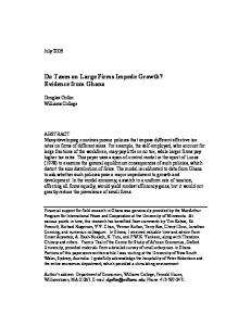
Figure 1: The effect of an increase in ⌦ on the market outcome

M⇤ =

2

"

F(fp + f )

1

s

fp fp + f

! # ⌦

N⇤ =

2

s

f 1+ fp

1

!

(15)

It is then easy to verify that the second condition (14) implies that for a given value of f , ¯ above which M ⇤ = 0: there is a threshold ⌦ p + f) ¯ = ⇣ F(fq ⌘ ⌦ fp 1 fp +f

This threshold is low when the cost of adding a new product fp is low. When there is such a decrease in per-product fixed costs, the barrier to entry f becomes relatively more important for SP firms, while MP firms benefit from this decrease on their whole product line. The market ¯ is enough to prevent entry and becomes more concentrated and thus a small number of firms ⌦ maintain a pure oligopoly. To put it differently, for a given ⌦ > 0, since M ⇤ is continuous in f , condition (14) holds as long as f is below a threshold f :

f=

✓

F(fp ) 1+ ⌦+1 19

◆2

!

1 fp

Figure 2: Typology of the market structure according to (f, ⌦) Proposition 2. An equilibrium exists featuring both types of firms iff

0 < f < f¯.

The couple (f, ⌦) defines a market structure that evolves from monopolistic competition, to a mixed market structure, and then on to oligopolistic competition, as represented in Figure 2. If there is no barrier to entry, and hence no economies of scope, MP-firms choose to be negligible N ⇤ = 0, so we are back to a market structure characterized by monopolistic competition. By contrast, as soon as f > 0, MP-firms have a positive mass in the economy and are thus able to impact market aggregates in the industry. Figure 2 shows that for a given number of oligopolists ⌦, when barriers to entry are prohibitive (f

f¯) the market structure is purely oligopolistic. Samely, for given barriers to entry, if

oligopolistic incumbents are too many, small firms do not enter and pure oligopoly is preserved. Comparative Statics w.r.t. Market Size and the Number of MP-Firms As expected, the mass of SP-firms decreases with the number of oligopolists; this effect is magnified when MP-firms can easily add a product to their product line (low fp ), so that they have a broader product scope, which increases their weight in the market. 20

When ⌦ is held constant, the mass of SP-firms increases with market size L, so that f¯ shifts up in Fig 2. When market size increases, both SP- and MP-firms benefit from a higher demand for their products but this may be offset by a decrease in their market power due to the intensification of competition both across and within the two types of firms. However, I show in this section that an SP-firm’s expected profit increases with market size which in turn drives entry, whereas the oligopolists’ profits do not depend on market size in the long run. More specifically, a direct consequence of (9) is that the number of products chosen by MP-firms does not depend on the number of oligopolists ⌦ or on market size L in the long run. Proposition 3. As long as both types of firms exist in equilibrium, the exogenous entry of an oligopolistic firm leads to the exit of monopolistic firms in the long run. Proposition 4. As long as both types of firm exist in equilibrium, an increase in the number of MP-firms leaves the product scope and profits of oligopolistic firms unchanged in the long run. The same result holds for an increase in market size. Since the mass of the competitive fringe adjusts so that the free entry condition holds again, the breadth of the product range is given by equation (15), which does not depend on ⌦ or L. Some intuition for these results can be provided with a decomposition of the short- and longrun effects. Before the competitive fringe adjusts to a change in ⌦, the scope of MP-firms varies following equation (10). For instance, when the number of MP-firms ⌦ increases, firms from the competitive fringe shrink in the short run as shown by (9), lowering their markup and sales. This, in turn, reduces their operating profit and makes them unable to incur the fixed cost to start producing. In the long run, the mass of the competitive fringe M decreases as expressed in (15). The exit of a range of SP-firms shifts demand towards both surviving SP-firms and MP-firms. They both raise their markups again and MP-firms increase their product range. In the end, (15) and (12) guarantee that MP-firms have exactly the same breadth of product range before and after entry of an extra oligopolist, while the surviving SP-firms produce exactly the same output. What is more, they make exactly the same profits as before. In the long run, the competitive fringe acts as a buffer that keeps the intensity of competition, proxied by X ⇤ , constant.16 This accounts for 16

While the idea that the long-run effects of free trade go against the short-run, pro-competitive effects remains

21

the persistence of large firms over time despite the important turnover of small firms. Under conditions (13), we can derive the firms’ (net) profit functions:

⇤ ⇡sp (X ⇤ )

⇧⇤! (X ⇤ )

N ⇤ (X ⇤ )fp =

fp + f = 0

4 ⇣p

fp + f

p ⌘2 fp > 0

The profits of MP-firms are independent from the number of oligopolists in the long run. Again, the pro-competitive effect due to an entry of an oligopolist is offset by the reallocation of market shares due to the exit of a range of SP-firms. Proposition 5. As long as both types of firm exist in equilibrium, the exogenous entry of an oligopolistic firm increases the total number of varieties unambiguously.

@V * = N⇤ @⌦

1

s

fp fp + f

!

>0

This variety effect is enabled because an MP-firm internalizes the consumers’ love for variety. Thus, a multi-product firm trades off a smaller output of each of its varieties against a broader product range. The output of each of its products is smaller than the output of an SP-firm. Altogether, the small firms behave like a multi-divisional firm producing a continuum of M products, ignoring their substitutability hence their cannibalization of each other.

Turning to welfare, continuum-quadratic preferences with a numeraire good lead to the following indirect utility: intuitive, the fact that they cancel each other out is an artefact from aggregative games featuring a one-dimensional statistic. Note that most models of trade under monopolistic competition admit a single aggregate statistic. Since the (exogenous) entry of a large firm has no impact on the incumbents’ product range, the results I have obtained yield a direct comparison with Shimomura and Thisse (2012) in which a firm’s mass is constant (and equal to one). They find that the entry of a large firm raises incumbent profits and output. As shown in Section 5 however, Proposition 4 holds true under their assumption of iso-elastic demand. The only difference stems from their assumption that the profits of large firms feed back into the demand level thereby generating a “market size” effect.

22

" # 1 E[↵ p]2 1 V⇤ U =R+ + V[p] 2 2 + V⇤ The entry of a big firm may affect consumer surplus through the average price level E[p] := 1 V

´

V

p⌫ d⌫, the price variance across varieties V[p] := E[p2 ]

E[p]2 and the total number of varieties

available to the consumer V. For a given number of varieties V, consumers value a low average price, i.e. U decreases with E[p], everything else being held constant. Consumers may also substitute a cheaper SP-firm variety for an MP-firm variety, the value of this trade-off is captured by V[p]. Last, for a given distribution of prices, consumers value the number of varieties V made available to them. In Appendix A, I show that the change in consumer surplus

CS following the entry of

one large firm is constant, negative, and equal to:

CS =

fp L

s

f 1+ fp

1

!2

Proposition 6. Consumer (producer) surplus decreases (increases) with the exogenous entry of a new oligopolist. All varieties produced by SP-firms which disappear are replaced by varieties supplied at a higher price by MP-firms. The average price E[p] unambiguously increases with ⌦ through a composition effect. Yet, this effect could be offset by the increase in V since consumers have a taste for variety. In general, the variety effect is dominated by the increase in the average price. The increase in the number of varieties together with an increase in the average price is at odds with the standard variety effect present in Krugman (1979), in which the availability of new varieties signifies that new firms have entered the market, hence there are lower prices (or a lower price-index if demand is iso-elastic). The change in the within-firm and across-firm extensive margins leads to opposite implications in terms of consumer surplus. The former margin means that there is more concentration and less competition, while the latter implies the opposite. The variety effect after the entry of a big firm fosters a transfer from consumer surplus to producer surplus. In Appendix A, I run a robustness check and consider a model in which a mass ⌦ of large firms are monopolistically competitive, but have higher prices because their product is perceived 23

as higher quality. The results are that the overall number of varieties decreases with ⌦, the average quality and price increase, but in the end the consumer surplus increases. This is taken as evidence that it is the source of a firm’s market power that matters for the distribution of welfare between consumers and producers. Social Welfare Under this particular specification of preferences, the entry of a large firm increases social welfare: profits increase more than the consumer surplus decreases. The consumers’ expenditures shift from the homogenous to the differentiated good, while at the same time the level of utility increases. The robustness of this result is discussed in Section 5.

3 3.1

Trade Openness to Trade and Firm Selection

I assume here that  symmetric countries are freely trading with each other and that conditions (13) and (14) for  = 1 are fullfilled. Following Eckel and Neary (2010), the openness to trade of each country is then measured by. This comes down to increasing the market size and the exogenous number of oligopolistic firms by a factor . Plugging the total market size L and the total number of MP-firms ⌦ in (14) and (15), the number of monopolistic firms under free entry for a given measure of openness  in each country can be derived:

M ⇤ () =

2 

"

F(; fp + f )

1

s

fp fp + f

!

⌦

#

(16)

with ↵ c F(; y) := q 2 Ly

1

Setting ⌦ = 0 in (16) leads to Krugman (1979)’s well-known result: monopolistically competitive firms enjoy economies of scale and consumers spread their consumption over a large set of varieties, 24

Figure 3: The effects of openness  on the size of the monopolistically competitive fringe M ⇤ thereby increasing the elasticity of demand so that firms reduce their markups.17 The number of varieties provided in each country decreases, but consumers enjoy a higher number of varieties overall: M ⇤ =

2 F (;fp +f )

· In other words, the mass of SP-firms is a concave and increasing

function of . On the contrary, given ⌦

1, the openness to trade also increases the number of large firms ⌦

which, following Proposition 3, triggers the exit of small firms. As shown in Figure 3.3 below, these two opposite effects lead to an inverted U-shaped curve for M : the market size effect itself decreases in  (consumers value new varieties less and less, so that F(; y) is a concave function of ), while the increase in the number of large firms is constant q ⇣ ⌘ fp and proportional to 1 ⌦, so that it eventually dominates. When economies of scope fp +f are large for MP-firms (high f ), the latter effect is stronger, as shown in Figure 3.

Regarding the total number of varieties, Proposition 5 guarantees that the overall number of varieties (SP- and MP-firms altogether) is an increasing function of the number of countries despite the exit of small firms. 17

This is a direct consequence of the elasticity of demand decreasing with individual consumption, a property which is true in the case of linear demand, but also assumed in Krugman (1979) for additively separable preferences.

25

3.2

Social Welfare

The variation of welfare with openness to trade is given by: dU @U @U =⌦ +L d @[⌦] @[L] Proposition 4 states that firm profits are independent from ⌦ and L. This means that the variation in the indirect utility U is given by the variation in consumer surplus only. Based on Proposition 6, an increase in the number of oligopolists raises the average price for differentiated goods, decreasing consumer surplus. Yet the effect of an increase in market size has a pro-competitive effect. Indeed, because SP-firms maintain their average-cost pricing rule, a higher market size translates into economies of scale, which lead to lower prices. This pro-competitive effect also operates for large firms: an increase in market size increases the output of large firms (see (8)), yet their profit remains constant (Proposition 4), meaning that large firms decrease their markup. To sum up, we have: Proposition 7. As long as both types of firms exist in equilibrium, an increase in the number of trading partners under free trade decreases the average price and increases the number of varieties available to consumers. In addition, consumer surplus and social welfare increase. In this section, we have shown that free trade opens the domestic market to more and more foreign exporters, which triggers the exit of small firms. In the absence of fixed costs to export (and thus no self-selection in the exporting activity), trade has a pro-competitive effect. Free trade allows small firms to export: in doing so, they maintain a tough competitive environment for big firms. As shown in the next section, there is a sharp constrast when firms self-select in the exporting activity in the presence of fixed costs.

4

Costly Trade Between Two Symmetric Countries

I now assume that in order to export a product to the foreign market, a firm must incur variable and fixed costs. Following the same logic as in the closed-economy section, first I derive some crosssection comparisons assuming a short-run equilibrium exists and taking the equilibrium large firm 26

product range as given. I then explore the role of fixed costs for selection and the long-run effects of trade liberalzation. The variable component of trade costs here is a per-unit additive18 trade cost ⌧ , so that the marginal cost of an exported variety is c + ⌧ .

4.1

A Cross-Section Comparison of MP- and SP-Firms in an Open Economy

Demand Since domestic and foreign countries are assumed to be of equal size, the analysis focuses on only one country. The inverse demand can be written again for any variety sold on the domestic market in quantity x to each consumer: p(x, X) = ↵

x

X

where X is the per-capita aggregated demand across products in one country. By symmetry, X gives an indication of the intensity of competition in each market: H H F F F F X = ⌦N H xH mp + M xsp + ⌦N xmp + M xsp | {z } Imported

varieties

The upperscripts H and F stand respectively for home and foreign markets. Production The foreign and domestic markets are segmented. Both small and large firms have a constant marginal cost of production. Furthermore, large firms have a constant marginal cost of adding a product, so both SP- and MP-firms make their decision independently on each market. 18

All results hold under “iceberg” trade costs.

27

The operating profits of foreign multi-product firms are then: ⇧Fmp

=

ˆ

NF

((pFmp

0

c

⌧ )LxFmp )dk

where pFmp is the cif -price of a variety. In the same way, the operating profits abroad of small firms are given by:

F ⇡sp = (pFsp

c

⌧ )LxFsp

Cross-Section Analysis The equilibrium value of X is taken as given and some cross-section comparisons between firms are derived, assuming both MP- and SP-firms export. Following Section 1.3, the output of large firms for the domestic and foreign markets can be derived:

Q⇤H mp (X) = L

N H (↵ c X) 2 + NH

Q⇤F mp (X, ⌧ ) = L

N F (↵ c ⌧ 2 + NF

X)

with density:

⇤H qmp (X) = L

↵ c X H 2 + N

⇤F qmp (X, ⌧ ) = L

↵

c 2 +

⌧

X

(17)

NF

⇤H ⇤H ⇤F ⇤F The output of an SP-firm is obtained for N F = N H = 0 in which case qmp = qsp and qmp = qsp .

At equilibrium, firm !’s absolute markups on the domestic and foreign market are given by the following expressions:

pH mp

1 c = (↵ + Q⇤H 2 L mp

X

c)

pFmp

1 c = (↵ + Q⇤F 2 L mp

X

c

⌧)

which yield a direct comparison with SP-firm markups:

pH sp

1 c = (↵ 2

X

c)

pFsp

1 c = (↵ 2

X

c

⌧)

so that exporters with a higher mass, or equivalently a higher output, charge higher prices by 28

adding higher markups. If both types of firms export, MP-firms charge higher prices than SPfirms.

4.2

Trade Liberalization

Fixed Costs To export, MP-firms face an overhead fixed cost fx . This fixed cost can be interpreted as in the standard Melitz model: firms need to establish a network or more generally look for buyers on the foreign market. Any additional variety exported on the foreign market requires an additional cost which can be interpreted as a packaging cost, or more generally as any other market-productspecific fixed cost. This cost is assumed to be equal to fp only for the sake of simplicity.19 Again, any form of heterogeneity within MP-firms is ruled out. The optimal product range on the domestic market is still given by (7). For exporting firms, it comes down to replacing c with c + ⌧ in the optimization program which yields a simple relation between the domestic and the exported product range:

N H⇤

NF⇤ =

⌧

s

L fp

When ⌧ decreases, it increases the marginal profit of exporting an additional variety, so that N F ⇤ ! N H⇤ . When ⌧ = 0, the per product profits are the same on the domestic and the foreign ⌧ !0

market, so that N F ⇤ = N H⇤ . Turning to SP-firms, they need to incur a total fixed cost equal to fp + fx in order to export their product. Once again, large firms spread fx on a continuum of varieties which they supply, so that the exporting activity fosters economies of scope. At the margin, it is easier for them to export a new product than it is for an SP-firm. Marginally, the cost of introducing a new product is fp for an MP-firm, and fp + fx for an SP-firm. Notice however that each large firm incurs a ´ NF⇤ total fixed cost of finite mass 0 fp + 1k=0 · fx dk. Thus, departing from the Melitz model, it is “immensely” greater than the fixed cost incurred by a small firm. 19

None of the results below rely on this assumption: a higher fixed cost per product to export would only further decrease the breadth of the exported product range.

29

Trade Liberalization: Comparative Statics w.r.t. to ⌧ A firm is an exporter if its profits abroad can cover the fixed cost of exporting. In the spirit of the Melitz model, I focus here on the case featuring selection into the exporting activity. This is the case when fixed costs are high enough.20 When there is no prospect of economies of scale, small firms choose not to export no matter what the extent of trade liberalization ⌧ > 0 is. However, the prospect of capturing rents abroad is a sufficient reason for MP-firms to export. Thus, there is a Nash equilibrium featuring selection between large and small firms. The algebra below is done for fx = f (see Footnote 20). MP-firms find it profitable to export when the following condition is verified: ⌧ < ⌧max := 2

r

(fp + f ) L

r

fp L

!

In the short run, holding the mass M of the competitive fringe constant, a decrease in ⌧ increases X, hence the intensity of competition. MP-firms lose some market shares on their domestic market (competition increases through the import penetration of foreign MP-firm varieties) and gain some new market shares through their exports. The mass of domestically-sold varieties Nd decreases and the mass of exported varieties Nx increases. This pattern is consistent with the well-documented intra-firm reallocation process of multi-product firms.21 From then on, any further drop in trade costs ⌧ only makes oligopolists more profitable. By contrast, SP-firms cannot compensate the increase in competitive pressure on the domestic market with their exporting activity since the latter is too costly. In the long run, SP-firms are forced to exit as trade liberalization occurs and there is a reallocation of their market shares towards the surviving firms: the market structure becomes more oligopolistic. The apparition of pure oligopoly depends upon the parameters of the model as shown in Figure 4. 20

A sufficient condition is fx f . When fx = f , a positive level of trade costs ⌧ guarantees that exporting is less profitable (including fixed costs) than domestic sales. Since small firms are free to enter and choose to export only if it is profitable, they never choose to do so. Intuitively, in the absence of economies of scale, small firms have no reason to export. 21 See Baldwin and Gu (2009); Bernard, Redding, and Schott (2011); Eckel, Iacovone, Smarzynska Javorcik, and Neary (2011) and Berthou and Fontagné, (forth.)

30

The Distribution of the Gains from Trade Comparing the market outcome under trade with the closed economy section, the intensity of competition X ⇤ at equilibrium is the same and determined by the free-entry condition on the domestic market for SP-firms.

⇤ ⇡sp (X ⇤ ) =

L (↵ 4

X ⇤ )2

c

(fp + f ) = 0

M ⇤ > 0 ) X ⇤ (⌧ ) = X ⇤ (⌧max ) = X ⇤ where X ⇤ is the equilibrium value of X in the absence of trade. Because the exporting activity is now costly, only large firms benefit from trade liberalization. Furthermore, small firms do not benefit from any efficiency gain as in the free-trade scenario. The exporting costs protect large firms to the extent that the competitive fringe cannot export. A decrease in trade costs does not increase competition in the long run. Indeed, the increase in competition because new varieties are imported is offset by the exit of SP-firms. MP-firms charge a lower markup on exported varieties: there is reciprocal dumping. Varieties that are exported are sold at the same price as varieties sold domestically.

⇤ F⇤ ⇤ pH⇤ mp (X ) = pmp (X ) = ↵

x⇤mp

X⇤

This implies in particular that even if MP-firms lose some market power in the short run due to a decrease in trade costs, their markup increases in the long run. While Brander and Krugman (1983) show that oligopolistic rents are driven down by a decrease in trade costs, a mixed market structure emphasizes the persistence of the market power of large firms so that, in the long run, there is no pro-competitive effect hurting the happy few MP-firms. To see how MP-firms gain from firm selection, their profit functions can be derived:

⇤ ⇧H mp (X )

Nd⇤ (X ⇤ )fp =

4 ⇣p fp + f

31

p ⌘2 fp

⇧Fmp (X ⇤ ; ⌧ )

N F ⇤ (X ⇤ ; ⌧ )fp =

4L

r

(fp + f ) L

r

fp L

!

⌧ 2

!2

=

L

(⌧max

⌧ )2

An interesting consequence of the adjustment of small firms is that the profits of MP-firms on the domestic market do not depend on trade costs. Once again, this is because any attempt to increase competition (increase in ⌦, decrease in ⌧ ) translates into the exit of SP-firms. The competitive fringe bears the long-run effects of trade liberalization alone. This is also to be compared with Brander and Krugman (1983) in which trade increases competition among oligopolists, whereas here the fringe absorbs the pro-competitive effect of trade liberalization in the long run. MP-firms make positive profits in equilibrium, which increase with a drop in trade costs and so does the average price of the differentiated good. Last, the overall number of varieties increases in spite of the exit of small firms. Proposition 8. Consumer (producer) surplus decreases (increases) when variable trade costs decrease. The increase in the number of varieties does not increase consumer surplus because new varieties are supplied at a higher price: large foreign firms gain more market power. It is worth stressing that such a prediction departs both from a pure monopolistic (Krugman, 1979) and from an oligopolistic (Brander, 1981) market structure. This shows how important it is to tackle the distribution of the gains from trade. Indeed, there is no monopolistic competition model which, by assumption, can account for the existence of positive profits in equilibrium. In such models, whether firms are heterogeneous or not, the sum of their short-run profits are mechanically passed on to the consumer surplus because of the free-entry condition. Last, it is important to keep in mind that these predictions hold under a mixed market structure only. As shown in Figure 4, a decrease in trade costs shifts the upper limit f¯ down.

32

Figure 4: Typology of the market structure with trade liberalization

5

Robustness

In this section, I explore the robustness of the previous results along several dimensions. Recent research has emphasized that the functional form assumed for the consumer demand system and preferences in models with monopolistic competition are not innocuous for positive and normative predictions (Dhingra and Morrow, 2012; Mrazova and Neary, 2012; Bertoletti and Epifani, 2012; Zhelobodko, Kokovin, Parenti, and Thisse, 2012). I also discuss other sources of firm heterogeneity.

5.1

Beyond Linear Demand

The current framework can be generalized assuming that inverse demand for a variety is of the ´ following form: p(x, ⇤) where x is still the consumption of a variety and ⇤ = V g(x⌫ )d⌫ is an aggregate statistic of a consumer’s consumption of all other varieties.22 All the results hold when g(.) is a strictly monotonic function and if ⇤ shifts the demand curve monotonically, e.g. p⇤ (x, ⇤) := @p (x, ⇤) @⇤

 0 8(x, ⇤) 2 R2+ . This specification includes linear demand, considered in the present

22

´ ˜ = The argument holds if the direct demand depends on a single statistic ⇤ g˜(p⌫ )d⌫. Therefore the results V obtained under quadratic preferences do not depend on whether firms compete in prices or in quantities.

33

paper with ⇤ = X =

´

V

x⌫ d⌫. It nests a large number of models of oligopolistic competition in the

industrial organization literature (see Etro, 2006), but also most demand systems used in the trade literature. For instance, additively separable preferences for the differentiated good in a partial equilibrium setting take the following form: U (A, x) = A + U (x) where U (x) = W

✓ˆ

0

V

u(x⌫ )d⌫

◆

where W and u(.) are assumed to be continously differentiable, increasing and concave. Inverse demand is then given by: p(x, ⇤) = u0 (x)W 0 (⇤) where ⇤=

ˆ

V

u(x⌫ )d⌫

0

Examples include Behrens and Murata (2007); Simonovska (2010) and CES preferences with elasticity of substitution 1 ´V ⇤ = 0 x⌫ d⌫.

> 1. In the latter case, ⇤ would take the familiar functional form

The demand system considered in this paper features a single aggregate ⇤ = X =

´V 0

x⌫ d⌫.

Firms impact competition toughness, proxied by ⇤ as soon as they supply a continuum of products with positive measure. As shown in Appendix C, large firms charge higher prices by adding higher markups (Proposition 1), and choose to be negligible if they do not benefit from economies of scope, i.e. f = 0 (Proposition 2). A large firm’s entry forces the monopolistically competitive fringe to shrink (Proposition 3), leaves large firms’ profits unchanged (Proposition 4) and increases the overall number of varieties (Proposition 5). Since the firms’ payoff depends on ⇤⇤ only, the total producer surplus increases linearly with the entry of a large firm.

34

5.2

Beyond Quadratic Preferences

I do not claim to make a general welfare analysis here, but I aim at least to check that my results are not driven entirely by the assumption of quadratic preferences. This section shows that the class of additively separable preferences may be treated with generality. This class of preferences displays enough flexibilty, as shown for instance by Kuhn-Vivès (1999) and Vivès (1999). The surplus analysis under this class of preferences is tractable because U (.) depends on ⇤ only. Variations in the consumer surplus are therefore driven by variations in expenditure. The consumer surplus can be expressed as follows: ⇤

CS := U (⇤ )

ˆ

V

p(⇤⇤ , x⌫ (⇤⇤ ))x⌫ (⇤⇤ )d⌫

0

With the notations introduced in the subsection above, U = W and g(x) = u(x) are increasing and concave. Note that consumer surplus is generally not a function of ⇤⇤ only; if it was, consumer surplus would remain constant.23 As shown in Appendix C, the change in consumer surplus with a large firm’s entry is:

where Eu =

u0 (x)x u(x)

⇥ 0 CS = N u(x⇤mp )W (⇤⇤ ) Eu (x⇤sp )

Eu (x⇤mp )

⇤

is the elasticity of the subutility u(.). I follow Kuhn and Vives (1999) and

assume that Eu is a decreasing function of individual consumption. This is the standard case, as it implies that “at low levels of total consumption a consumer cares less about variety increases (relative to total output increases) than at high consumption levels”. Therefore the change in consumer surplus is negative. The change in social welfare is ambiguous however. Indeed, a higher consumer surplus comes at the cost of the multi-product technology, i.e. the fixed cost fp which is incurred by large firms for each product. Even if producing one variety is more efficient when undertaken by a large firm rather than by a small firm (Proposition 2), large firms may still produce too many varieties, i.e. the marginal gain from selling a new variety for an MP-firm may be smaller than the decrease it 23

See Anderson, Erkal, and Piccinin (2013) for a detailed review of games and demand systems which satisfy this property.

35

entails for consumer surplus. Whether one or the other dominates is generally ambiguous and depends on the functional forms assumed for the utility function, together with the importance of economies of scope. Note that if large firms behaved like multi-divisional firms, they would charge a price equal to the one charged by small firms. In that case, social welfare would always increase with a large firm’s entry thanks to economies of scope. When they behave strategically, the only case which is not ambiguous is when economies of scope are very low, i.e. f = 0+ . In that case again, MP-firms behave like multi-divisional firms, so that a large firm’s entry always raises social welfare (see Appendix C). To sum up, I have shown that my results regarding the distribution of the gains from trade between consumers and producers are robust to a large class of functional forms. However, even if the level of social welfare increases under continuum-quadratic preferences and CES preferences as in Shimomura and Thisse (2012), it need not be so, even for well-behaved preferences.24 If large firms did not behave strategically, social welfare would always increase.

5.3

Firm Heterogeneity

There are many dimensions along which firms may differ. Here, we have assumed that MP-firms are more efficient because they benefit from economies of scope. One may wonder how the results are affected when MP-firms are assumed to have a lower marginal cost of production than SPfirms, so that cmp < csp . In this case, most results are unaffected as the total output value remains unchanged and determined by (12). MP-firms would have a broader product range, but still higher prices than small firms. From a social welfare perspective, differences in marginal costs, in addition to economies of scope, tend to make the use of labor more efficient, so that social welfare is now more likely to rise with a large firm’s entry. Secondly, this paper has assumed that a discrete number of a few happy firms are born with a multi-product technology. On the contrary, models à la Mélitz in the trade literature usually assume that firms become heterogeneous after they incur a sunk cost, then drawing their produc24

Counter-examples include functional forms which belong to the HARA family.

36

tivity from a given distribution. While this approach has proved successful to model heterogeneity under monopolistic competition, I want to emphasize here that it is not enough to model a mixed market structure. Consider the following reductio ad absurdum argument: assume that, in the spirit of Melitz (2003), firms draw their productivity parameter from a distribution function with a c.d.f.

(.). Assume further that there exists a productivity cutoff '⇤ above which firms choose to

enter and a productivity cutoff '⇤mp > '⇤ above which ⌦⇤ MP-firms may choose to be of positive mass. Then, in order to have a mixed market structure, there must be a positive mass M ⇤ > 0 of SP-firms with productivity ranging from '⇤ to '⇤mp . This implies in turn that there is a positive mass of entrants ME⇤ :=

M⇤ . ('⇤mp ) ('⇤ )

But if there is such a continuum of entrants, there is also

a positive mass of MP-firms equal to ME⇤ 1

('⇤mp ) . This means that MP-firms are negligible

and thus unable to impact market aggregates, which ends the argument. Thus, the path taken in this paper should be seen as a simple alternative.

6

Concluding Remarks

Consistent with the empirical evidence that a few large, long-lasting players are responsible for most trade flows, I have built a model with a “mixed” market structure in which a few multiproduct oligopolists and a continuum of single-product monopolistically competitive firms coexist. I have shown that ex-ante firm heterogeneity appears endogenously at equilibrium as a necessary condition for the coexistence of both types of firm. Because firm heterogeneity is addressed in terms of firm behavior, the reallocation of the market shares of exiting firms which follows a drop in bilateral trade costs uncovers a channel that affects intra-industry competition and consumer surplus negatively. When barriers to trade select the largest firms into exporting, bilateral liberalization under a mixed market structure may have an anti-competitive effect rather than a pro-competitive one. The average price in the industry increases as its market structure becomes oligopolistic. This model emphasizes that a higher concentration on the supply side of the economy transfers the gains from trade from consumers to firms. Last, this paper complements the literature emphasizing heterogeneity in product appeal across 37

firms. Such an explanation is crucial to explain why small firms may still export or be relatively less hurt by globalization than their larger counterparts (Holmes and Stevens, forth.). Nevertheless, I believe that the predictions derived in this paper show that it is important to put strategic interactions back into trade theory.

38

References Anderson, S. P., N. Erkal, and D. Piccinin (2013): “Aggregate Oligopoly Games with Entry,” CEPR Discussion Papers. Baldwin, J., and W. Gu (2009): “The impact of trade on plant scale, production-run length and diversification,” in producer dynamics: New Evidence from micro data, pp. 557–592. University of Chicago Press. Baldwin, R. E., and G. I. Ottaviano (1998): “Multiproduct Multinationals and Reciprocal FDI Dumping,” Discussion paper, National Bureau of Economic Research. Behrens, K., and Y. Murata (2007): “General equilibrium models of monopolistic competition: a new approach,” Journal of Economic Theory, 136(1), 776–787. Bernard, A., J. Jensen, S. Redding, and P. Schott (2007): “Firms in international trade,” The Journal of Economic Perspectives, 21(3), 105–130. Bernard, A. B., S. J. Redding, and P. K. Schott (2011): “Multiproduct firms and trade liberalization,” The Quarterly Journal of Economics, 126(3), 1271–1318. Berthou, A., and L. Fontagné (2013): “How do Multiproduct Exporters React to a Change in Trade Costs?,” Scandinavian Journal of Economics (forthcoming). Bertoletti, P., and P. Epifani (2012): “Monopolistic Competition: CES Redux?,” Discussion paper, University of Pavia, Department of Economics and Management. Brander, J. (1981): “Intra-industry trade in identical commodities,” Journal of International Economics, 11(1), 1–14. Brander, J., and P. Krugman (1983): “A reciprocal dumping’model of international trade,” Journal of International Economics, 15(3-4), 313–321. Brander, J. A., and B. J. Spencer (1985): “Export subsidies and international market share rivalry,” Journal of International Economics, 18(1), 83–100. 39

Breinlich, H., and C. Criscuolo (2011): “International trade in services: A portrait of importers and exporters,” Journal of International Economics, 84(2), 188–206. Crozet, M., D. Mirza, and E. Millet (2010): “The Ultra-Select Club of Service Export Firms,” La Lettre du CEPII, (302). Dhingra, S. (2013): “Trading Away Wide Brands for Cheap Brands,” American Economic Review (forthcoming). Dhingra, S., and J. Morrow (2012): “Monopolistic Competition and Optimum Product Diversity Under Firm Heterogeneity,” London School of Economics, mimeo. Dixit, A., and V. Norman (1980): Theory of international trade: A dual, general equilibrium approach. Cambridge University Press. Eaton, J., and G. M. Grossman (1986): “Optimal trade and industrial policy under oligopoly,” The Quarterly Journal of Economics, 101(2), 383–406. Eckel, C., L. Iacovone, B. Smarzynska Javorcik, and J. Neary (2011): “Multi-product firms at home and away: Cost-versus quality-based competence,” CEPR Discussion Papers, (8186). Eckel, C., and J. Neary (2010): “Multi-product firms and flexible manufacturing in the global economy,” Review of Economic Studies, 77(1), 188–217. Etro, F. (2006): “Aggressive leaders,” The RAND Journal of Economics, 37(1), 146–154. Feenstra, R., and H. Ma (2008): “Optimal Choice of Product Scope for Multiproduct Firms, oforthcoming in (eds) Elhanan Helpman, Dalia Marin and Thierry Verdier, The Organization of Firms in a Global Economy,” . Friedman, J. (1993): Oligopoly theory, vol. 2 of Handbook of Mathematical Economics. Elsevier. Hart, O. D. (1985): “Monopolistic competition in the spirit of Chamberlin: A general model,” The Review of Economic Studies, 52(4), 529–546. 40

Holmes, T., and J. Stevens (2013): “An alternative theory of the plant size distribution with an application to trade,” Journal of Political Economy (forthcoming). Krugman, P. (1979): “Increasing returns, monopolistic competition, and international trade,” Journal of international Economics, 9(4), 469–479. Kuhn, K.-U., and X. Vives (1999): “Excess entry, vertical integration, and welfare,” The RAND Journal of Economics, pp. 575–603. Manova, K., and Z. Zhang (2009): “China’s exporters and importers: Firms, products and trade partners,” NBER Working Paper 15249. Manova, K., and Z. Zhang (2012): “Export prices across firms and destinations,” The Quarterly Journal of Economics, 127(1), 379–436. Markham, J. W. (1951): “The Nature and Significance of Price Leadership,” The American Economic Review, 41(5), 891–905. Markusen, J. R. (1981): “Trade and the gains from trade with imperfect competition,” Journal of international economics, 11(4), 531–551. Mayer, T., M. Melitz, and G. Ottaviano (2013): “Market size, competition and the product mix of exporters,” American Economic Review (forthcoming). Mayer, T., and G. Ottaviano (2008): “The happy few: the internationalisation of European firms,” Intereconomics, 43(3), 135–148. Melitz, M. (2003): “The impact of trade on intra-industry reallocations and aggregate industry productivity,” Econometrica, pp. 1695–1725. Melitz, M., and G. Ottaviano (2008): “Market size, trade, and productivity,” Review of Economic studies, 75(1), 295–316. Mrazova, M., and J. P. Neary (2012): “Selection Effects with Heterogeneous Firms,” CEPR Discussion Papers, (9288). 41

Neary, P. (2009): “International Trade in General Oligopolistic Equilibrium,” mimeo. (2010): “Two and a Half Theories of Trade,” World Economy, 33(1), 1–19. Ottaviano, G. I., and J.-f. Thisse (2011): “Monopolistic competition, multiproduct firms and optimum product diversity,” The Manchester School, 79(5), 938–951. Redding, S. J. (2011): “Theories of Heterogeneous Firms and Trade,” Annual Review of Economics, 3(1), 77–105. Roberts, J., and H. Sonnenschein (1977): “On the foundations of the theory of monopolistic competition,” Econometrica: Journal of the Econometric Society, pp. 101–113. Salant, S., S. Switzer, and R. Reynolds (1983): “Losses from horizontal merger: the effects of an exogenous change in industry structure on Cournot-Nash equilibrium,” The Quarterly Journal of Economics, 98(2), 185. Shimomura, K., and J. Thisse (2012): “Competition among the big and the small,” The RAND Journal of Economics, 43(2), 329–347. Simonovska, I. (2010): “Income differences and prices of tradables,” National Bureau of Economic Research. Vives, X. (1999): Oligopoly pricing: old ideas and new tools. MIT press. Zhelobodko, E., S. Kokovin, M. Parenti, and J. Thisse (2012): “Monopolistic competition in general equilibrium: Beyond the C.E.S.,” Econometrica, 80(6), 2765–2784.

42

Large and Small Firms in a Global Market: David vs. Goliath Supplementary Material Mathieu Parenti⇤

A. Consumer Surplus A.1 Variations of Consumer Surplus with the Number of Large Firms Each consumer’s surplus is:

CS := ↵X

2

ˆ

V

0

x2⌫ d⌫

X2

2

ˆ

V

p⌫ x⌫ d⌫

0

where X=

ˆ

V

x⌫ d⌫

0

When small firms can enter and exit freely and as long as both types of firms exist, X ⇤ , x⇤mp , x⇤sp and N ⇤ do not depend on ⌦. Thus, the change in consumer surplus following the entry of one large firm is:

CS = where

⌦N x2mp +

2

M x2sp

M is the mass of SP-firms which exit following this entry. It can be derived from (15):

M= ⇤ CORE

2

2

1

s

fp fp + f

!

- Université Catholique de Louvain, Belgium E-mail: [email protected]

1

and thus CS =

2

xmp (xmp

qxp )

Therefore, plugging the equilibrium value of N ⇤ , we get a simple expression for the change in consumer surplus which can be simplified as follows: fp L

CS =

s

f 1+ fp

!2

1

⇤

A.2 Variations in Consumer Surplus: Monopolistically Competitive Firms with Higher Quality. Assume the existence of two groups of firms: a continuum of M firms and a continuum of ⌦ firms, both competing monopolistically with only M-type firms being governed by a free-entry condition, while the mass ⌦ is exogenous. In order to draw a comparison with the model, assume that consumers have are more willing to pay for varieties1 supplied by the “monopolsitically competitive large firms”. Their preferences can be written as follows:

U = ↵!

ˆ

⌦

xi di + ↵

0

ˆ

M

xj dj

2

0

ˆ

0

V

ˆ

x2⌫ d⌫

V

x⌫ d⌫

0

!2

This yields the following demand system:

p! = ↵ !

x!

X

pm = ↵

xm

X

The consumption of each variety can be derived: xsp (X ⇤ ) =

↵

c 2

X⇤

xmp (X ⇤ ) =

↵!

c 2

X⇤

⌦-firms will charge a higher price than M firms iff ↵! > ↵. From there, the implications of an exogenous entry of ⌦-firms for welfare are direct: using the algebra developed in A.1, we get: 1 Notice

that whether ⌦ firms are single-product or multi-product firms in this exercise does not make a difference.

2

CS =

2

x⇤mp x⇤mp

x⇤sp

Therefore the entry of a large firm increases consumer surplus. This happens because the nature of the market power in the two models is different. In the original model, the fact that large firms charge a higher markup is only the consequence of their strategic behavior.

B. Positive Consumption of the Numeraire and the Differentiated Goods. For the differentiated goods to be consumed at equilibrium in a mixed market structure, consumers must be willing to pay ↵ and/or the market size must be large enough for firms to cover their fixed cost of entry. This condition is already present in the equilibrium condition (14). However, for the numeraire good to be consumed at equilibrium, ↵ (resp.

) should not be too high (too

low) in order to make sure that consumer income is not entirely spent on the differentiated good. The total spending on the differentiated good is: ˆ

V

0

p⇤⌫ x⇤⌫ d⌫ = M ⇤ p⇤sp x⇤sp + ⌦N ⇤ p⇤mp x⇤mp

and each consumer’s income is 1 +

⌦⇧⇤ mp L .

Thus, we have to make sure that:

1 > M ⇤ p⇤sp x⇤sp + ⌦N ⇤ cx⇤mp + fp Using equations (5), (8), (12) and (15), the expressions of M ⇤ , p⇤sp , p⇤mp and N ⇤ can be plugged into the right-hand side term. A direct inspection shows that it is decreasing in ⌦. A sufficient condition is thus that the inequality holds when there are no large firms: ⇤ 1 > M⌦=0 p⇤sp x⇤sp

1>

2

F(fp + f ) c

s

3

fp + f + fp + f L

!

where F(y) :=

↵

c 2

s

L y

1

so this holds when

1>

2

"

↵

c 2

s

L (fp + f )

1

#

c

s

fp + f + fp + f L

!

which can be rearranged as

↵<

q

(fp +f ) L

⇣ q ⌘ +c+2 fp +f c + f + f p L

r

(fp + f ) L

is assumed to be large enough for the expression above to hold. Since the two equilibrium conditions (13) and (14) do not depend on , it ensures positive consumption of the numeraire good at any equilibrium.

C. Robustness Positive Predictions Each firm faces an inverse demand function p(x, ⇤), where ⇤ =

´

V

g(xi )di is an aggregate statistic,

where g is a strictly increasing function with g(0) = 0. Each firm faces a downward sloping demand curve, so that px < 0. Notice that the same approach can be considered for competition ˜ where ⇤ ˜ = à la Bertrand with a differentiated good, writing the direct demand function x(p, ⇤), ´ g˜(xi )di. Without loss of generality, I deal with the Cournot case to ease the comparison with V the model.

If a firm has a product range of positive mass, then its decisions impact ⇤ directly. ⇤ is the relevant statistic which describes competition toughness for firms, an increase in ⇤ is assumed to shift the demand curve down, i.e. p⇤ (x, ⇤)  0 8x

0. I assume that the functional forms

chosen for p(., .) and g(.) are twice differentiable and such that the existence and uniqueness of an equilibrium is guaranteed. k=N

The first-order condition for an MP-firm with respect to (x!k )k=1 ! , conditional upon N! leads to:

4

0

px x!k + g (x!k )

ˆ

N!

p⇤ (x!k , ⇤)dk

0

!

+p

c=0

which is to be compared with the first-order condition for an SP-firm:

px xsp + p

c=0

x!k does not depend on k, so x! := x!k and thus the first-order condition for MP-firms is again: px x! + N! g 0 (x! )p⇤ + p

c=0

Therefore, since the marginal revenue px x + p of SP-firms decreases with x, we get that x⇤! decreases with N . Hence prices increase with N , generalizing proposition 1. ⇤ Let us note x

!

⇤

the vector of equilibrium consumption from all firms but firm !. Firm !’s

profits are a function of ⇤ and x (firms play an aggregative game with a single statistic ⇤). The equilibrium value of firm !’s density of profits ⇡!⇤ is defined as:

⇡!⇤ := max ⇡(x! , ⇤(x! , x x! 0

!

⇤

)

This is to be compared with the profit of an SP-firm: ⇤ ⇡sp := max ⇡(xm , ⇤⇤ (x⇤! , x xm 0

!

⇤

))

where x⇤! := Argmax[⇧! ] which implies that

⇤ ⇡sp

⇡(x⇤! , ⇤(x⇤! , x

!

⇤

)) = ⇡!⇤

Assuming symmetry among large firms again, the subscript mp is used instead of ! so: ⇤ ⇡sp

⇤ ⇡mp

This expression emphasizes the “free-riding” of small firms off the strategic behavior of large

5

firms. Everything else being equal, large firms try to decrease ⇤ to relax competition, which benefits to all ⇤-taking firms. Equality holds only when MP-firms are negligible, i.e. N ⇤ = 0. Economies of scope ensure that it is profitable for large firms to have a positive mass, generalizing Proposition 2.2 ⇤ Since x⇤m decreases monotonically with ⇤ and since p⇤  0, ⇤⇤ has been assumed to be uniquely determined by the free-entry condition: p(x⇤sp (⇤⇤ ), ⇤⇤ )

c x⇤sp (⇤⇤ ) = fp + f

Therefore if there is an equilibrium, ⇤⇤ does not depend on ⌦. Since the first-order condition for large firms implies that x⇤mp depends on ⇤⇤ only, it does not depend on ⌦ either. The first-order condition with respect to N holds true at equilibrium: g(xmp )⇤ p⇤ (x⇤mp , ⇤⇤ )N ⇤ x⇤mp + (p(x⇤mp , ⇤⇤ )

c)x⇤mp = fp

Thus, if there eixsts an optimal and finite product range N ⇤ , then it depends on ⌦ only through ⇤⇤ . Therefore N ⇤ remains unchanged when comparative statics w.r.t. ⌦ are drawn. Since by definition ⇤⇤ = ⌦N ⇤ g(x⇤mp ) + M ⇤ g(x⇤sp ), M ⇤ must decrease, generalizing Proposition 3. ⇤ The same argument generalizes Proposition 4 ⇤. Last, since x⇤mp < x⇤sp and g(.) is increasing, for ⇤⇤ to remain constant with an increase in ⌦, the overall number of varieties ⌦N ⇤ + M ⇤ must increase, generalizing Proposition 5. ⇤

Normative Predictions Consumer Surplus If U (.) depends on ⇤ only, then CS is simply a function of V: CS := U (⇤⇤ ) Using the fact that ⇤⇤ =

´V 0

ˆ

V

p(⇤⇤ , x⌫ (⇤⇤ ))x⌫ (⇤⇤ )d⌫

0

g(x⇤⌫ )d⌫ does not depend on ⌦, the change in consumer surplus

2 Notice that this argument does not rely on the functional form taken by ⇤, or on the assumption that it is a scalar. It holds true in particular even in general equilibrium.

6

with the entry of a large firm is:

CS =

 N ⇤ p⇤mp x⇤mp

g(x⇤mp ) ⇤ ⇤ p x g(x⇤sp ) sp sp

Under additively separable preferences, g(x) = u(x) and 0

p(x, ⇤) = u0 (x)W (⇤) so the change in consumer surplus is: ⇥ 0 CS = N ⇤ u(x⇤mp )W (U ) Eu (x⇤m )

Eu (x⇤mp )

⇤

which generalizes Propositions 6 and 8. Social Welfare: General Case The change in total producer surplus following the entry of one large firm equals its profits: ⇣ 0 P S = N ⇤ u0 (x⇤mp )x⇤mp W (⇤⇤ ) that is PS = N

⇤

0 u(x⇤mp )W

⇤

(⇤ )

✓

Eu (x⇤mp )

cx⇤mp

fp

⌘

cx⇤mp + fp u(x⇤mp )W 0 (⇤⇤ )

◆

Thus the change in social welfare is:

CS +

PS = N

⇤

0 u(x⇤mp )W

⇤



(⇤ ) Eu (x⇤m )

cx⇤mp + fp u(x⇤mp )W 0 (⇤⇤ )

The first-order condition w.r.t. N can be used: 00

(p⇤mp

c)x⇤mp + u(x⇤mp )u0 (x⇤mp )W (⇤⇤ )N ⇤ x⇤mp =

fp L

so 0

"

CS+ P S = N ⇤ u(x⇤mp )W (⇤⇤ ) Eu (x⇤sp )

0

00

u0 (x⇤mp )W (⇤⇤ )x⇤mp + u(x⇤mp )u0 (x⇤mp )W (⇤⇤ )N ⇤ x⇤mp u(x⇤mp )W 0 (⇤⇤ )

7

#

CS +

⇥ 0 P S = N ⇤ u(x⇤mp )W (⇤⇤ ) Eu (x⇤sp )

Eu (x⇤mp )

EW 0 (x⇤mp )

⇤

where EW 0 (x⇤mp ) reflects the change in expenditure. This expression can be further simplified using the ratio of the first-order conditions for both firms: u0 (x⇤mp ) 1 + Eu0 (x⇤sp ) = > 1 where u0 (x⇤sp ) 1 + Eu0 (x⇤sp ) + EW 0 (x⇤mp )

Eu0 (y) =

u00 (y)y u0 (y)

so that the change in social welfare can be written:

CS +

 0 P S = N u(x⇤mp )W (⇤⇤ ) Eu (x⇤sp )

Eu (x⇤mp ) + 1

Eu0 (x⇤mp ) + 1

Eu0 (x⇤sp )

u0 (x⇤sp ) u0 (x⇤mp )

And we already know that x⇤mp < x⇤sp . However, this expression can be positive or negative. For instance, if u(x) = (1 + x)↵

1 with ↵ < 1 and if f is not too small, then the entry of a large

firm decreases social welfare. Social Welfare: f = 0+ Note that: 0

(Eu ) = If f is small enough, then x⇤sp get

CS +

u0 [1 u

E u0

Eu ] 0

x⇤mp is close to zero. In the standard case, i.e. (Eu ) < 0, we

P S > 0. ⇤

8