Learning hierarchical invariant spatio-temporal features for action recognition with independent subspace analysis Quoc V. Le, Will Y. Zou, Serena Y. Yeung, Andrew Y. Ng Computer Science Department and Department of Electrical Engineering, Stanford University [email protected], [email protected], [email protected], [email protected]

Abstract

pendent Component Analysis (ICA), both very well-known in the field of natural image statistics [10, 41]. Experimental studies in this field have shown that these algorithms can learn receptive fields similar to the V1 area of visual cortex when applied to static images and the MT area of visual cortex when applied to sequences of images [10, 40, 32]. An advantage of ISA, compared to the more standard ICA algorithm, is that it learns features that are robust to local translation while being selective to frequency, rotation and velocity. A disadvantage of ISA, as well as ICA, is that it can be very slow to train when the dimension of the input data is large. In this paper, we scale up the original ISA to larger input data by employing two important ideas from convolutional neural networks [19]: convolution and stacking. In detail, we first learn features with small input patches; the learned features are then convolved with a larger region of the input data. The outputs of this convolution step are inputs to the layer above. This convolutional stacking idea enables the algorithm to learn a hierarchical representation of the data suitable for recognition [22]. We evaluate our method using the experimental protocols described in Wang et al. [42] on four well-known benchmark datasets: KTH [37], Hollywood2 [26], UCF (sport actions) [35] and YouTube [23]. Surprisingly, despite its simplicity, our method outperforms all published methods that use either hand-crafted [42, 23] or learned features [39] (see Table 1). The improvements on Hollywood2 and YouTube datasets are approximately 5%.

Previous work on action recognition has focused on adapting hand-designed local features, such as SIFT or HOG, from static images to the video domain. In this paper, we propose using unsupervised feature learning as a way to learn features directly from video data. More specifically, we present an extension of the Independent Subspace Analysis algorithm to learn invariant spatio-temporal features from unlabeled video data. We discovered that, despite its simplicity, this method performs surprisingly well when combined with deep learning techniques such as stacking and convolution to learn hierarchical representations. By replacing hand-designed features with our learned features, we achieve classification results superior to all previous published results on the Hollywood2, UCF, KTH and YouTube action recognition datasets. On the challenging Hollywood2 and YouTube action datasets we obtain 53.3% and 75.8% respectively, which are approximately 5% better than the current best published results. Further benefits of this method, such as the ease of training and the efficiency of training and prediction, will also be discussed. You can download our code and learned spatio-temporal features here: http://ai.stanford.edu/∼wzou/

1. Introduction Common approaches in visual recognition rely on handdesigned features such as SIFT [24, 25] and HOG [4]. A weakness of such approaches is that it is difficult and timeconsuming to extend these features to other sensor modalities, such as laser scans, text or even videos. There is a growing interest in unsupervised feature learning methods such as Sparse Coding [31, 21, 34], Deep Belief Nets [7] and Stacked Autoencoders [2] because they learn features directly from data and consequently are more generalizable. In this paper, we provide further evidence that unsupervised learning not only generalizes to different domains but also achieves impressive performance on many realistic video datasets. At the heart of our algorithm is the use of Independent Subspace Analysis (ISA), an extension of Inde-

Table 1. Our results compared to the best results so far on four datasets (See Table 2, 3, 4, 5 for more detailed comparisons). KTH Hollywood2 UCF YouTube Best published 92.1% 50.9% 85.6% 71.2% results Our results 93.9% 53.3% 86.5% 75.8%

The proposed method is also fast because it requires only matrix vector products and convolution operations. In our timing experiments, at prediction time, the method is as fast as other hand-engineered features. 3361

2. Previous work

as, Sparse Coding [31], Independent Component Analysis (ICA) [9] and Independent Subspace Analysis [8] have long been studied by researchers in the field of natural image statistics. There has been a growing interest in applying these methods to learn visual features. For example, Raina et al. [33] demonstrate that sparse codes learned from unlabeled and unrelated tasks can be very useful for recognition. They name this approach “self-taught learning.” Further, Kanan and Cottrell [13] show that ICA can be used as a self-taught learning method to generate saliency maps and features for robust recognition. They demonstrate that their biologically-inspired method can be very competitive in a number of datasets such as Caltech, Flowers and Faces. In [18], TICA, another extension of ICA, was proposed for static images that achieves state-of-the-art performance on NORB [20] and CIFAR-10 [15] datasets. Biologically-inspired networks [11, 39, 12] have been applied to action recognition tasks. However, except for the work of [39], these methods have certain weaknesses such as using hand-crafted features or requiring much labeled data. For instance, all features in Jhuang et al. [11] are carefully hand-crafted. Similarly, features in the first layer of [12] are also heavily hand-tuned; higher layer features are adjusted by backpropagation which requires a large amount of labeled data (see the Conclusion section in [12]). In contrast, our features are learned in a purely unsupervised manner and thus can leverage the plethora of unlabeled data.

In recent years, low-level hand-designed features have been heavily employed with much success. Typical examples of such successful features for static images are SIFT [24, 25], HOG [4], GLOH [27] and SURF [1]. Extending the above features to 3D is the predominant methodology in video action recognition. These methods usually have two stages: an optional feature detection stage followed by an feature description stage. Well-known feature detection methods (“interest point detectors”) are Harris3D [16], Cuboids [5] and Hessian [43]. For descriptors, popular methods are Cuboids [5], HOG/HOF [17], HOG3D [14] and Extended SURF [43]. Some other interesting approaches are proposed in [38, 30]. Given the current trends, challenges and interests in action recognition, this list will probably grow rapidly. In a very recent work, Wang et al. [42] combine various low-level feature detection, feature description methods and benchmark their performance on KTH [37], UCF sports action [35] and Hollywood2 [26] datasets. To make a fair comparison, they employ the same state-of-the-art processing pipeline with Vector Quantization, feature normalization and χ2 -kernel SVMs. The only variable factor in the pipeline is the use of different methods for feature detection and feature extraction. One of their most interesting findings is that there is no universally best hand-engineered feature for all datasets; their finding suggests that learning features directly from the dataset itself may be more advantageous. In our paper, we will follow Wang et al. [42]’s experimental protocols by using their standard processing pipeline and only replacing the first stage of feature extraction with our method. By doing this, we can easily understand the contributions of the learned features. Recently, a novel convolutional GRBM method [39] was proposed for learning spatio-temporal features. This method can be considered an extension of convolutional RBMs [22] to 3D. In comparison to our method, their learning procedure is more expensive because the objective function is intractable and thus sampling is required. As a consequence, their method takes 2-3 days to train with the Hollywood2 dataset [26].1 This is much slower than our method which only takes 1-2 hours to train. Our method is therefore more practical for large scale problems. Furthermore, our experimental procedure is different from one proposed by Taylor et al. [39]. Specifically, in Taylor et al. [39], the authors create a pipeline with novel pooling mechanisms – sparse coding, spatial average pooling and temporal max pooling. The two new factors, learned features coupled with the new pipeline, make it difficult to assess the contributions of each stage. Biologically-inspired sparse learning algorithms such 1 Personal

3. Algorithms and Invariant Properties In this section, we will first describe the basic Independent Subspace Analysis algorithm which is often used to learn features from static images. Next, we will explain how to scale this algorithm to larger images using convolution and stacking and learn hierarchical representations. Also, in this section, we will discuss batch projected gradient descent. Finally, we will present a technique to detect interest points in videos.

3.1. Independent subspace analysis for static images ISA is an unsupervised learning algorithm that learns features from unlabeled image patches. An ISA network [10] can be described as a two-layered network (Figure 1), with square and square-root nonlinearities in the first and second layers respectively. The weights W in the first layer are learned, and the weights V of the second layer are fixed to represent the subspace structure of the neurons in the first layer. Specifically, each of the second layer hidden units pools over a small neighborhood of adjacent first layer units. We will call the first and second layer units simple and pooling units, respectively. More precisely, given an input pattern xt , the activation of each second layer unit is pi (xt ; W, V ) = qP Pn m t 2 k=1 Vik ( j=1 Wkj xj ) . ISA learns parameters W through finding sparse feature representations in the second

communications with G. Taylor.

3362

Figure 3. Tuning curves for ISA pooling units when trained on static images. The x-axes are variations in translation/frequency/rotation, the y-axes are the normalized activations of the network. Left: change in translation (phase). Middle: change in frequency. Right: change in rotation. These three plots show that pooling units in an ISA network are robust to translation and selective to frequency and rotation changes.

Figure 1. The neural network architecture of an ISA network. The red bubbles are the pooling units whereas the green bubbles are the simple units. In this picture, the size of the subspace is 2: each red pooling unit looks at 2 simple units.

layer, by solving: minimize

PT

subject to

WW

W

Pm

t=1 T

i=1

=I

pi (xt ; W, V ),

(1)

In many experiments, we found that this invariant property makes ISA perform much better than other simpler methods such as ICA and sparse coding.

where {xt }Tt=1 are whitened input examples.2 Here, W ∈ Rk×n is the weights connecting the input data to the simple units, V ∈ Rm×k is the weights connecting the simple units to the pooling units (V is typically fixed); n, k, m are the input dimension, number of simple units and pooling units respectively. The orthonormal constraint is to ensure the features are diverse. In Figure 2, we show three pairs of filters learned from natural images. As can be seen from this figure, the ISA algorithm is able to learn Gabor filters (“edge detectors”) with many frequencies and orientations. Further, it is also able to group similar features in a group thereby achieving invariances.

3.2. Stacked convolutional ISA The standard ISA training algorithm becomes less efficient when input patches are large. This is because an orthogonalization method has to be called at every step of projected gradient descent. The cost of the orthogonalization step grows as a cubic function of the input dimension (see Section 3.4). Thus, training this algorithm with high dimensional data, especially video data, takes days to complete. In order to scale up the algorithm to large inputs, we design a convolutional neural network architecture that progressively makes use of PCA and ISA as sub-units for unsupervised learning as shown in Figure 4. The key ideas of this approach are as follows. We first train the ISA algorithm on small input patches. We then take this learned network and convolve with a larger region of the input image. The combined responses of the convolution step are then given as input to the next layer which is also implemented by another ISA algorithm with PCA as a prepossessing step. Similar to the first layer, we use PCA to whiten the data and reduce their dimensions such that the next layer of the ISA algorithm only works with low dimensional inputs. In our experiments, the stacked model is trained greedily layerwise in the same manner as other algorithms proposed in the deep learning literature [7, 2, 22]. More specifically, we train layer 1 until convergence before training layer 2. Using this idea, the training time requirement is reduced to 1-2 hours.

Figure 2. Typical filters learned by the ISA algorithm when trained on static images. Here, we visualize three groups of bases produced by W (each group is a subspace and pooled together).

One property of the learned ISA pooling units is that they are invariant and thus suitable for recognition tasks. To illustrate this, we train the ISA algorithm on natural static images and then test its invariance properties using the tuning curve test [10]. In detail, we find the optimal stimulus of a particular neuron pi in the network by fitting a parametric Gabor function to the filter. We then vary its three degrees of freedom: translation (phase), rotation and frequency and plot the activations of the neurons in the network with respect to the variation. 3 Figure 3 shows results of the tuning curve test for a randomly selected neuron in the network with respect to spatial variations. As can be seen from this figure, the neuron is robust to translation (phase) while being more sensitive to frequency and rotation. This combination of robustness and selectivity makes features learned by ISA highly invariant [6]. 2 I.e.,

3.3. Learning spatio-temporal features Applying the models above to the video domain is rather straightforward: the inputs to the network are 3D video blocks instead of image patches. More specifically, we take mean and identity covariance. 3 In this test, we use image patches of a typical size 32x32.

the input patterns have been linearly transformed to have zero

3363

1

W to the constraint set by computing (W W T )− 2 W . Note that the inverse square root of the matrix usually involves solving an eigenvector problem, which requires cubic time. Therefore, this algorithm is expensive when the input dimension is large. The convolution and stacking ideas address this problem by slowly expanding the receptive fields via convolution. And although we have to resort to PCA for whitening and dimension reduction, this step is called only once and hence much less expensive. Training neural networks is difficult and requires much tuning. Our method, however, is very easy to train because batch gradient descent does not need any tweaking with the learning rate and the convergence criterion. This is in stark contrast with other methods such as Deep Belief Nets [7] and Stacked Autoencoders [2] where tuning the learning rate, weight decay, convergence parameters, etc. is essential for learning good features.

Figure 4. Stacked Convolutional ISA network. The network is built by “copying” the learned network and “pasting” it to different places of the input data and then treating the outputs as inputs to a new ISA network. For clarity, the convolution step is shown here non-overlapping, but in the experiments the convolution is done with overlapping.

a sequence of image patches and flatten them into a vector. This vector becomes input features to the network above. To learn high-level concepts, we can use the convolution and stacking techniques (see Section 3.2) which result in an architecture as shown in Figure 5.

3.5. Norm-thresholding interest point detector In many datasets, an interest point detector is necessary for improving recognition and lowering computational costs. This can be achieved in our framework by discarding features at locations where the norm of the activations is below a certain threshold. This is based on the observation that the first layer’s activations tend to have significantly higher norms at edge and motion locations than at static and feature-less locations (c.f. [13]). Hence, by thresholding the norm, the first layer of our network can be used as a robust feature detector that filters out features from the non-informative background: If kp1 (xt ; W, V )k1 ≤ δ then the features at xt are ignored. here p1 is the activations of the first layer of the network. For instance, setting δ at 30 percentile of the training set’s activation norms means that 70% of features from the dataset are discarded. In our experiments, we only use this detector the KTH dataset where an interest point detector has been shown to be useful [42]. The value of δ is chosen via cross validation.

Figure 5. Stacked convolutional ISA for video data. In this figure, convolution is done with overlapping; the ISA network in the second layer is trained on the combined activations of the first layer.

Finally, in our experiments, we combine features from both layers and use them as local features for classification (previously suggested in [22]). In the experiment section, we will show that this combination works better than using one set of features alone.

In Section 3.1, we discussed spatial invariant properties of ISA when applied to image patches. In this section, we extend the analysis for video bases.

3.4. Learning with batch projected gradient descent

4.1. First layer

Our method is trained by batch projected gradient descent. Compared to other feature learning methods (e.g., RBMs [7]), the gradient of the objective function in Eq. 1 is tractable. The orthonormal constraint is ensured by projection with symmetric orthogonalization [10]. In detail, during optimization, projected gradient descent requires us to project

The first layer of our model learns features that detect a moving edge in time as shown in Figure 6. In addition to previously mentioned spatial invariances, these spatiotemporal bases give rise to another property: velocity selectivity. We analyze this property by computing the response of ISA features while varying the velocity of the moving edge.

4. Feature visualization and analysis

3364

directions than other directions. 90 60

120

Figure 6. Examples of three ISA features learned from Hollywood2 data (16x16 spatial size). In this picture, each row consists of two sets of filters. Each set of filters is a filter in 3D (i.e., a row in matrix W ), and two sets grouped together to form an ISA feature.

30

150

180

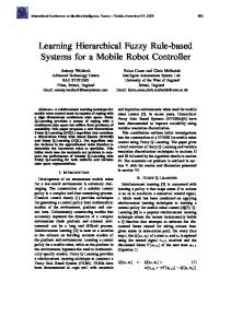
In detail, we fit Gabor functions to all temporal bases to estimate the velocity of the bases. We then vary this velocity and plot the response of the features with respect to the changes. In Figure 7, we visualize this property by plotting the velocity tuning curves of five randomly-selected units in the first layer of the network.

0

210

330

240

300 270

Figure 8. A polar plot of edge velocities (radius) and orientations (angle) to which filters give maximum response. Each red dot in the figure represents a pair of (velocity, orientation) for a spatiotemporal filter learned from Hollywood2. The outermost circle has velocity of 4 pixels per frame.

4.2. Higher layers

Figure 7. Velocity tuning curves of five neurons in a ISA network trained on Hollywood2. Most of the tuning curves are unimodal and this means that ISA temporal bases can be used as velocity detectors.

Figure 9. Visualization of five typical optimal stimuli in the second layer learned from Hollywood2 data (for the purpose of better visualization, we use the size of 24x24x18 built on top of 16x16x10 first layer filters). Compare this figure with Figure 6

As can be seen from the figure, the neurons are highly sensitive to changes in the velocity of the stimuli. This suggests that the features can be used as velocity detectors which are valuable for detecting actions in movies. For example, the “Running” category in Hollywood2 has fast motions whereas the “Eating” category in Hollywood2 has slow motions. Informally, we can interpret filters learned with our ISA model as features detecting a moving edge through time. In particular, the pooling units are sensitive to motion – how fast the edge moves – and also sensitive to orientation but less sensitive to (translational) locations of the edge. We found that the ability to detect accurate velocities is very important for good recognition. In a control experiment, we limit this ability by using a temporal size of 2 frames instead of 10 frames and the recognition rate drops by 10% for the Hollywood2 dataset. Not only can the bases detect velocity, they also adapt to the statistics of the dataset. This ability is shown in Figure 8. As can be seen from the figure, for Hollywood2, the algorithm learns that there should be more edge detectors in vertical and horizontal orientations than other orientations. Informally, we can interpret that the bases spend more effort to detect velocity changes in the horizontal and vertical

Figure 10. Comparison of layer 1 filters (left) and layer 2 filters (right) learned from Hollywood2. For ease of visualization, we ignore the temporal dimension and only visualize the middle filter.

Visualizing and analyzing higher layer units are usually difficult. Here, we follow [3] and visualize the optimal stimuli of the higher layer neurons.4 Some typical optimal stimuli for second layer neurons are shown in Figure 9 and 4 In detail, the method was presented for visualizing optimal stimuli of neurons in a quadratic network for which the corresponding optimization problem has an analytical solution. As our network is not quadratic, we have to solve an optimization problem subject to a norm bound constraint of the input. We implement this with minConf [36].

3365

(93.9%) and the closest competitive method (92.1%).5

Figure 10. Although the learned features are more difficult to interpret, the visualization suggests they have complex shapes (e.g., corners [22]) and invariances suitable for detecting high-level structures.

Table 2. Average accuracy on the KTH dataset. The symbol (**) indicates that the method uses an interest point detector. Our method is the best with the norm-thresholding interest point detector. Algorithm Accuracy (**) Harris3D [16] + HOG/HOF [17] (from [42]) 91.8% (**) Harris3D [16] + HOF [17] (from [42]) 92.1% (**) Cuboids [5] + HOG3D [14] (from [42]) 90.0% Dense + HOF [17] (from [42]) 88.0% (**) Hessian [43] + ESURF [43] (from [42]) 81.4% HMAX [11] 91.7% 3D CNN [12] 90.2% (**) pLSA [29] 83.3% GRBM [39] 90.0% Our method with Dense sampling 91.4% (**) Our method with norm-thresholding 93.9%

5. Experiments In this section we will numerically compare our algorithm against the current state-of-the-art action recognition algorithms. We would like to emphasize that for our method we use an identical pipeline as described in [42]. This pipeline extracts local features, then performs vector quantization by K-means and classifies by χ2 kernel. With our method, the only change is the feature extraction stage: we replaced hand-designed features with the learned features. Results of control experiments such as speed, benefits of the second layer and training features on unrelated data [33] are also reported. Further results, detailed comparisons and parameter settings can be seen in the Appendix (http://ai.stanford.edu/∼wzou/).

Table 3. Mean AP on the Hollywood2 dataset. Algorithm Mean AP Harris3D [16] + HOG/HOF [17] (from [42]) 45.2% Cuboids [5] + HOG/HOF [17] (from [42]) 46.2% Hessian [43] + HOG/HOF [17] (from [42]) 46.0% Hessian [43] + ESURF [43] (from [42]) 38.2% Dense + HOG/HOF [17] (from [42]) 47.7% Dense + HOG3D [14] (from [42]) 45.3% GRBM [39] 46.6% Our method 53.3%

5.1. Datasets We evaluate our algorithm on four well-known benchmark action recognition datasets: KTH [37], UCF sport actions [35], Hollywood2 [26] and YouTube action [23]. These datasets were obtained from original authors’ websites. The processing steps, dataset splits and metrics are identical to those described in [42] or [23]. The main purpose of using identical protocols is to identify the contributions of the learned features.

Table 4. Average accuracy on the UCF sport actions dataset. Algorithm Accuracy Harris3D [16] + HOG/HOF [17] (from [42]) 78.1% Cuboids [5] + HOG3D [14] (from [42]) 82.9% Hessian [43] + HOG/HOF [17] (from [42]) 79.3% Hessian [43] + ESURF [17] (from [42]) 77.3% Dense + HOF [17] (from [42]) 82.6% Dense + HOG3D [14] (from [42]) 85.6% Our method 86.5%

5.2. Details of our model For our model, the inputs to the first layer are of size 16x16 (spatial) and 10 (temporal). Our first layer ISA network learns 300 features (i.e., there are 300 red nodes in Figure 1). The inputs to the second layer are of size 20x20 (spatial) and 14 (temporal). Our second layer ISA network learns 200 features (i.e., there are 200 red nodes in the last layer in Figure 4). Finally, we train the features on 200000 video blocks sampled from the training set of each dataset.

Table 5. Average accuracy on the YouTube action dataset. Algorithm Accuracy Feature combining and pruning [23]: 71.2% - Static features: HAR + HES + MSER [28] + SIFT [25] - Motion features: Harris3D [16] + Gradients + PCA + Heuristics Our method 75.8%

5.3. Results We report the performance of our method on the KTH dataset in Table 2. In this table, we compare our test set accuracy against best reported results in literature. More detailed results can be seen in [42] or [12]. We note that for this dataset, an interest point detector can be very useful because the background does not convey any meaningful information [42]. Therefore, we apply our norm-thresholding interest point detector to this dataset (see Section 3.5). Using this technique, our method achieves superior performance compared to all published results in the literature. There is an increase in performance between our method

A comparison of our method against best published results for Hollywood2 and UCF sport actions datasets is reported in Table 3 and 4. In these experiments, we only consider dense sampling for our algorithm. As can be seen from the tables, our approach outperforms a wide range of 5 Our model achieves 94.5% if we use the interest point detector to filter out the background, then run feature extraction more densely than described in [42].

3366

methods. The performance improvement, in case of the challenging Hollywood2 dataset, is significant: 5%. Finally, in Table 5, we report the performance of our algorithm on the YouTube actions dataset [23]. The results show that our algorithm outperforms a more complicated method [23] on the dataset by a margin of 5%.

of the comparison are given in Table 6.

5.6. Self-taught learning In previous experiments, we trained our features on the given training set. For instance, in Hollywood2, we trained spatio-temporal features on the training split of 823 videos. The statistics of the data on which features are trained are similar to statistics of the test data. An interesting question to consider, is how the model performs when the unsupervised learning stage is carried out on unrelated video data, for instance, videos downloaded from the Internet. This is the Self-taught learning paradigm [33]. To answer this question, we trained the convolutional ISA network on small video blocks randomly sampled from UCF and Youtube datasets. Using the learned model, we extract features from Hollywood2 video clips and run the same evaluation metric. Under this self-taught setting, the model achieves 51.1% AP on Hollywood2. While this setting performs less well than learning directly from the training set (53.3%), it is still better than prior art results reported in Wang et. al [42]. The encouraging result illustrates the ability of our method to learn useful features for classification using widely-available unlabeled video data.

5.4. Benefits of the second layer In the above experiments, we combine features from layer 1 and layer 2 for classification. This raises a question: How much does the second layer help? To answer this question, we rerun the experiments with the same settings and discard second layer’s features. The results are much worse than previous experiments. More specifically, removing the second layer features results in a significant drop of 3.05%, 2.86%, 4.12% in terms of accuracy on KTH, UCF and Hollywood2 datasets respectively. This confirms that features from the second layer are indeed very useful for recognition.

5.5. Training and prediction time Unsupervised feature learning is usually computationally expensive, especially in the training phase. For instance, the GRBM method, proposed by [39], takes around 2-3 days to train.6 In contrast, for the training stage, out algorithm takes 1-2 hours to learn the parameters on 200000 training examples using the setting in Section 5.2.7 Feature extraction using our method is very efficient and as fast as hand-designed features. In the following experiment, we compare the speed of our method and HOG3D [14] during feature extraction.8 This comparison is obtained by extracting features with dense sampling on 30 video clips with a framesize of 360x288 from the Hollywood2 dataset.

6. Conclusion In this paper, we presented a method that learns features from spatio-temporal data using independent subspace analysis. We scaled up the algorithm to large receptive fields by convolution and stacking and learn hierarchical representations. Experiments were carried out with KTH, Hollywood2, UCF sports action and YouTube datasets using a very standard processing pipeline [42]. Using this pipeline, we observed that our simple method outperforms many state-ofthe-art methods. This result is interesting, given that our single method, using the same parameters across four datasets, is consistently better than a wide variety of combinations of methods. It also suggests that learning features directly from data is a very important research direction: Not only is this approach more generalizable to many domains, it is also very powerful in recognition tasks.

Table 6. Feature extraction time. Our method with 2 layers on GPU is 2x faster than HOG3D. Algorithm Seconds/Frame Speed× HOG3D [14] 0.22 base Our method (1 layer) 0.14 1.6× Our method (2 layers) 0.44 0.5× Our method (2 layers, GPU) 0.10 2.2×

The results show that if we use one layer, our method is faster than HOG3D. But if we use two layers, our algorithm is slower than HOG3D. However, as our method is dominated by matrix vector products and convolutions, it can be implemented and executed much more efficiently on a GPU. Our simple implementation on a GPU (GTX 470) using Jacket9 enjoys a speed-up of 2x over HOG3D. Details

Acknowledgments: We thank Zhenghao Chen, Adam Coates, Pang Wei Koh, Fei-Fei Li, Jiquan Ngiam, Juan Carlos Niebles, Andrew Saxe, Graham Taylor for comments and suggestions. This work was supported by the DARPA Deep Learning program under contract number FA8650-10C-7020.

6 Personal

communications with G. Taylor. timing experiments are done with a machine with 2.26GHz CPU and 24Gb RAM. 8 Provided on the author’s website. 9 http://www.accelereyes.com/

References

7 The

[1] H. Bay, A. Ess, T. Tuytelaars, and L. V. Gool. Speeded up robust features. In CVIU, 2008. 3362

3367

SURF:

[2] Y. Bengio, P. Lamblin, D. Popovici, and H. Larochelle. Greedy layerwise training of deep networks. In NIPS, 2006. 3361, 3363, 3364 [3] P. Berkes and L. Wiskott. Slow feature analysis yields a rich repertoire of complex cell properties. Journal of Vision, 2005. 3365 [4] N. Dalal and B. Triggs. Histograms of oriented gradients for human detection. In CVPR, 2005. 3361, 3362 [5] P. Dollar, V. Rabaud, G. Cottrell, and S. Belongie. Behavior recognition via sparse spatio-temporal features. In VS-PETS, 2005. 3362, 3366 [6] I. Goodfellow, Q. Le, A. Saxe, H. Lee, and A. Ng. Measuring invariances in deep networks. In NIPS, 2010. 3363 [7] G. Hinton, S. Osindero, and Y. Teh. A fast learning algorithms for deep belief nets. Neu. Comp., 2006. 3361, 3363, 3364 [8] A. Hyvarinen and P. Hoyer. Emergence of phase- and shiftinvariant features by decomposition of natural images into independent feature subspaces. Neu. Comp., 2000. 3362 [9] A. Hyvarinen and P. Hoyer. Topographic independent component analysis as a model of v1 organization and receptive fields. Neu. Comp., 2001. 3362 [10] A. Hyvarinen, J. Hurri, and P. Hoyer. Natural Image Statistics. Springer, 2009. 3361, 3362, 3363, 3364 [11] H. Jhuang, T. Serre, L. Wolf, and T. Poggio. A biologically inspired system for action recognition. In ICCV, 2007. 3362, 3366 [12] S. Ji, W. Xu, M. Yang, and K. Yu. 3D convolutional neural networks for human action recognition. In ICML, 2010. 3362, 3366 [13] C. Kanan and G. Cottrell. Robust classification of objects, faces, and flowers using natural image statistics. In CVPR, 2010. 3362, 3364 [14] A. Klaser, M. Marszalek, and C. Schmid. A spatio-temporal descriptor based on 3D gradients. In BMVC, 2008. 3362, 3366, 3367 [15] A. Krizhevsky. Learning multiple layers of features from tiny images. Technical report, U. Toronto, 2009. 3362 [16] I. Laptev and T. Linderberg. Space-time interest points. In ICCV, 2003. 3362, 3366 [17] I. Laptev, M. Marszalek, C. Schmid, and B. Rozenfeld. Learning realistic human actions from movies. In CVPR, 2008. 3362, 3366 [18] Q. V. Le, J. Ngiam, Z. Chen, D. Chia, P. W. Koh, and A. Y. Ng. Tiled convolutional neural networks. In NIPS, 2010. 3362 [19] Y. LeCun and Y. Bengio. Convolutional networks for images, speech, and time- series. The Handbook of Brain Theory and Neural Networks, 1995. 3361 [20] Y. LeCun, F. Huang, and L. Bottou. Learning methods for generic object recognition with invariance to pose and lighting. In CVPR, 2004. 3362 [21] H. Lee, A. Battle, R. Raina, and A. Y. Ng. Efficient sparse coding algorithms. In NIPS, 2007. 3361 [22] H. Lee, R. Grosse, R. Ranganath, and A. Ng. Convolutional deep belief networks for scalable unsupervised learning of hierarchical representations. In ICML, 2009. 3361, 3362, 3363, 3364, 3366

[23] J. Liu, J. Luo, and M. Shah. Recognizing realistic actions from videos “in the Wild”. In CVPR, 2009. 3361, 3366, 3367 [24] D. Lowe. Object recognition from local scale-invariant features. In ICCV, 1999. 3361, 3362 [25] D. Lowe. Distinctive image features from scale-invariant keypoints. In IJCV, 2004. 3361, 3362, 3366 [26] M. Marzalek, I. Laptev, and C. Schmid. Actions in context. In CVPR, 2009. 3361, 3362, 3366 [27] K. Mikolajczyk and C. Schmid. A performance evaluation of local descriptors. PAMI, 27(10):1615–1630, 2005. 3362 [28] K. Mikolajczyk, T. Tuytelaars, C. Schmid, A. Zisserman, J. Matas, F. Schaffalitzky, T. Kadir, and L. V. Gool. A comparison of affine region detectors. IJCV, 2004. 3366 [29] J. Niebles, H. Wang, and L. Fei-Fei. Unsupervised learning of human action categories using spatial-temporal words. IJCV, 2008. 3366 [30] A. Oikonomopoulos, I. Patras, and M. Pantic. Spatiotemporal salient points for visual recognition of human actions. IEEE Trans. Systems, Man, and Cybernetics, 2006. 3362 [31] B. Olshausen and D. Field. Emergence of simple-cell receptive field properties by learning a sparse code for natural images. Nature, 1996. 3361, 3362 [32] B. A. Olshausen. Sparse coding of time-varying natural images. In ICA, 2000. 3361 [33] R. Raina, A. Battle, H. Lee, B. Packer, and A. Ng. Selftaught learning: Transfer learning from unlabelled data. In ICML, 2007. 3362, 3366, 3367 [34] R. Raina, A. Madhavan, and A. Y. Ng. Large-scale deep unsupervised learning using graphics processors. In ICML, 2009. 3361 [35] M. Rodriguez, J. Ahmed, and M. Shah. Action mach: A spatio-temporal maximum average correlation height filter for action recognition. In ICCV, 2008. 3361, 3362, 3366 [36] M. Schmidt. minConf, 2005. 3365 [37] C. Schuldt, I. Laptev, and B. Caputo. Recognizing human actions: A local SVM approach. In ICPR, 2004. 3361, 3362, 3366 [38] H. J. Seo and P. Milanfar. Detection of human actions from a single example. In ICCV, 2009. 3362 [39] G. Taylor, R. Fergus, Y. Lecun, and C. Bregler. Convolutional learning of spatio-temporal features. In ECCV, 2010. 3361, 3362, 3366, 3367 [40] J. van Hateren and D. Ruderman. Independent component analysis of natural image sequences yields spatio-temporal filters similar to simple cells in primary visual cortex. Proceedings of the Royal Society: Biological Sciences, 1998. 3361 [41] J. van Hateren and D. Ruderman. Independent component filters of natural images compared with simple cells in primary visual cortex. Proc Royal Society, 1998. 3361 [42] H. Wang, M. M. Ullah, A. Klaser, I. Laptev, and C. Schmid. Evaluation of local spatio-temporal features for action recognition. In BMVC, 2010. 3361, 3362, 3364, 3366, 3367 [43] G. Willems, T. Tuytelaars, and L. V. Gool. An efficient dense and scale-invariant spatio-temporal interest point detector. In ECCV, 2008. 3362, 3366

3368