JOURNAL OF GUIDANCE, CONTROL, AND DYNAMICS Vol. 33, No. 2, March–April 2010
Low-Thrust Transfers in the Earth–Moon System, Including Applications to Libration Point Orbits M. T. Ozimek∗ and K. C. Howell† Purdue University, West Lafayette, Indiana 47907-2045 DOI: 10.2514/1.43179 Preliminary designs of low-thrust transfer trajectories are developed in the Earth–moon three-body problem with variable specific impulse engines and fixed engine power. The solution for a complete time history of the thrust magnitude and direction is initially approached as a calculus of variations problem to locally maximize the final spacecraft mass. The problem is then solved directly by sequential quadratic programming, using either single or multiple shooting. The coasting phase along the transfer exploits invariant manifolds and, when possible, considers locations along the entire manifold surface for insertion. Such an approach allows for a nearly propellant-free final coasting phase along an arc selected from a family of known trajectories that contract to the periodic libration point orbit. This investigation includes transfer trajectories from an Earth parking orbit to some sample libration point trajectories, including L1 halo orbits, L1 and L2 vertical orbits, and L2 butterfly orbits. Given the availability of variable specific impulse engines in the future, this study indicates that fuel-efficient transfer trajectories could be used in future lunar missions, such as south pole communications satellite architectures.
Subscripts
Nomenclature c G H Isp i m P R r, v
= = = = = = = = =
S T t U uc u^ T X �^ � � �M � �M �
= = = = = = = = = = = = = = = = =
� $, �
constraint vector endpoint function Hamiltonian engine specific impulse instantaneous inclination angle total spacecraft mass engine power magnitude rotation matrix position and velocity vectors, Earth–moon rotating frame design variable vector engine thrust magnitude time pseudopotential function control vector thrust direction unit vector uncontrolled state vector, Earth–moon rotating frame eigenvector at a fixed point on a periodic orbit control constraint Lagrange multiplier vector instantaneous argument of latitude anglelike manifold parameter costate vector timelike manifold parameter state transition matrix kinematic boundary condition vector instantaneous right ascension angle kinematic boundary condition Lagrange multiplier vectors
c f FP MS p PO s SS u 0
= = = = = = = = = =
control variable final condition fixed point condition multiple shooting phase powered phase parking orbit condition stable manifold single shooting phase unstable manifold initial condition
I. Introduction
W
ITHIN the last 25 years, libration point orbits have emerged as a valuable trajectory alternative for spacecraft mission design. Beginning with the launch of the International Sun–Earth Explorer (ISEE-3) on 12 August 1978 and its successful direct transfer into a sun–Earth L1 halo orbit [1], libration point orbits are now viable options for suitable scientific applications. More recently, an interest in a return to the moon has prompted trajectory design studies for several new mission objectives, including the development of continuous communications links [2–6]. Satellites in orbits that ensure lunar south pole coverage are one such example that has received attention as a possible new application for libration point orbits [3–6]. Accessing these orbits ultimately requires a means of transfer from an Earth parking orbit. One approach is through highly efficient lowthrust propulsion. This technology has been demonstrated as a primary source of propulsion in missions, such as Deep Space 1 [7] and the Small Missions for Advanced Research in Technology (SMART-1) [8]. The difficulty in constructing low-thrust trajectories is, of course, the computation of a long-duration thrust magnitude and direction history. Typically, these unknown parameters are specified as part of a trajectory optimization problem to locally maximize or minimize a performance index, such as final spacecraft mass or total burn time. Investigations to solve these optimization problems have become an area of intense study, and they are typically classified in terms of either direct or indirect methods. (A useful survey of each method is discussed by Betts [9], with four methods also discussed by Hull [10]). In addition to being classified as direct/ indirect, another important distinction between the existing solution methods is the decision to employ explicit or implicit numerical integration.
Presented as Paper 343 at the 2007 AAS/AIAA Astrodynamics Specialist Conference, Mackinac Island, MI, 19–23 August 2007; received 12 January 2009; revision received 1 October 2009; accepted for publication 13 October 2009. Copyright © 2009 by M. T. Ozimek and K. C. Howell. Published by the American Institute of Aeronautics and Astronautics, Inc., with permission. Copies of this paper may be made for personal or internal use, on condition that the copier pay the $10.00 per-copy fee to the Copyright Clearance Center, Inc., 222 Rosewood Drive, Danvers, MA 01923; include the code 0731-5090/10 and $10.00 in correspondence with the CCC. ∗ Ph.D. Candidate, School of Aeronautics and Astronautics, Armstrong Hall of Engineering, 701 West Stadium Avenue. Student Member AIAA. † Hsu Lo Professor of Aeronautical and Astronautical Engineering, School of Aeronautics and Astronautics, Armstrong Hall of Engineering, 701 West Stadium Avenue. Associate Fellow AIAA. 533
534
OZIMEK AND HOWELL
Indirect methods involve the two-point boundary value problem (TPBVP) that arises from the calculus of variations formulation, and they traditionally involve explicit numerical integration. The TPBVP introduces unknown costates, necessary to parameterize the controls, and additional optimality constraint equations. Compared with most direct methods, solving the TPBVP indirectly (often via indirect shooting [11–13]) involves relatively few unknown parameters that are each highly sensitive, especially given the long propagation times and nonlinear dynamics. Despite this difficulty, indirect methods often exhibit rapid convergence when compared with a direct method and generally require significantly fewer function evaluations when implemented with a numerical root-solving procedure. Many early research investigators focused on indirect solutions [14–17]. Although many current efforts use direct approaches, several relatively recent studies [11–13] have returned to indirect approaches due to the benefits of adjoint control transformations (ACTs) [18] and the low dimensions required to set up the problem. Because guesses for the initial costates are so often problematic in solving a TPBVP, multiple shooting [19,20] was introduced as a means to decompose a trajectory into a series of segments and partition the sensitivities over many nodes. This method has been successfully demonstrated in several low-thrust problems [21,22]. Multiple shooting also allows the addition of kinematic constraints to the nodes joining each trajectory segment. Direct methods typically convert the calculus of variations problem into a parameter optimization problem, in which a scheme such as nonlinear programming (NLP) is employed to minimize the performance index. Single and multiple shooting methods may also serve in so-called hybrid formulations, in which components of the TPBVP are established to continuously parameterize the control via explicit integration [22–25]. Rather than satisfy all optimality constraints, the cost function is instead minimized. Many direct methods transcribe the states, and sometimes the controls, through implicit integration. These methods include direct transcription/ collocation [26–29] and differential inclusion [30,31]. In these direct approaches, the entire trajectory is represented in terms of nodes, and a large number of design variables are used to increase the convergence radius, sometimes removing the costate variables completely. Static/dynamic control is another direct method that has been developed for high-fidelity simulation [32]. Yet again, many design variables are required to parameterize a long-duration transfer, and many function evaluations are required. The preceding indirect and direct approaches characterize a variety of local optimization techniques. There often exist many local extrema to the performance index in a given problem. In such cases, global optimization procedures may be employed to further improve a solution from a local method. Whereas the software to compute a local optimum is typically a gradient-based procedure, many globally optimizing algorithms (such as genetic algorithms) are stochastic. In trajectory design, genetic algorithms have been applied with notable success to gravitational flyby solutions, which involve an extraordinary number of feasible and locally optimal possibilities [33,34]. Global methods often involve significant computational expense and require feasible or locally optimal solutions that can be rapidly generated. In this investigation, emphasis is placed on local solutions, because the resulting long-duration Earth escape portions of the trajectories are highly sensitive and require a significant amount of compute time to even obtain a single solution. In general, few low-thrust investigations have focused on transfers to libration point orbits. Gómez et al. [35] and Howell et al. [36] developed transfer trajectories via the stable manifold with impulsive maneuvers in the sun–Earth/moon system. Starchville and Melton [37,38] used a dynamical systems approach and combined a thrust arc with a naturally convergent coast to a libration point orbit. They employed a tangent steering law to determine the fuel optimal insertion onto individual manifolds in the Earth–moon circularrestricted and elliptic-restricted problem. Sukhanov and Eismont [39] developed a transfer to a sun–Earth L2 halo orbit by calculating a spiral trajectory within a two-body model, and then they determined the finite burns necessary to replicate an optimal two-burn impulsive transfer in the three-body system. Many researchers (for example,
Kluever and Pierson [23,24] and Herman and Conway [28]) incorporated the restricted three-body problem as a precursor to higherfidelity gravitational models, but they did not focus on transfers to libration point orbits. Senent et al. [40] considered the benefits of exposing the stable invariant manifold behavior along the entire surface of a given periodic orbit in the sun–Earth/moon system. Their low-thrust transfer trajectories also employed a variable specific impulse (VSI) engine model and a detailed calculus of variations approach that used a primer vector control law. Similarly, Mingotti et al. [41] considered transfers to halo orbits in the Earth–moon problem with a direct transcription and collocation approach, using constant specific impulse engines. Their results also included subsequent transfer trajectories departing the halo orbits. A recent study also considered constant specific impulse engine transfers to unstable manifolds at Europa in an ephemeris model [42]. This investigation considers the benefits of using the stable invariant manifolds to produce preliminary low-thrust transfer designs within the Earth–moon system. Similar to Senent et al. [40], an indirect formulation is initially established within the context of the calculus of variations to transfer a spacecraft from an Earth parking orbit to the stable manifold, with the spacecraft asymptotically coasting to the desired orbit upon insertion. Instead of solving the complete TPBVP, a hybrid approach is used, and the transversality conditions are foregone in favor of obtaining a direct solution. This method is selected to maintain a relatively low number of design variables yet widen the convergence radius. Both direct single shooting and direct multiple shooting [9] are employed to minimize a performance index of final spacecraft mass using a VSI engine model. As an extension of a previous study by Grebow et al. [5], several target trajectories are considered, including L1 halo orbits, L1 and L2 vertical orbits, and L2 butterfly orbits.
II. A.
Uncontrolled System Models
Equations of Motion
The uncontrolled spacecraft motion is assumed to be subject to the dynamics in the Earth–moon circular restricted three-body problem (CR3BP). The primary gravitational bodies (Earth and moon) move about their barycenter on circular paths. The third body (i.e., the spacecraft) is assumed to possess negligible mass in comparison with the primaries. The rotating x^ axis is defined along the vector between the primaries; the z^ axis is parallel to the angular velocity vector associated with the Keplerian primary orbits. Then, the usual barycentric system of equations, describing the motion of the third body, are written compactly in terms of position r and velocity v as � � @U�r� T � h�v� (1) r� � @r where the dots indicate the nondimensional time derivatives relative to an observer in the rotating frame, and the acceleration vectors include the pseudopotential gradient @U�r� and the kinematic velocity @r function h�v�; that is, 2 3 x � �1 � ���x � ��=d13 � ��x � 1 � ��=d23 T @U�r� 6 7 �4 y � �1 � ��y=d13 � �y=d23 5 @r ��1 � ��z=d13 � �z=d23 2 3 2y_ 6 7 h�v� � 4 �2x_ 5 (2) 0 The values of x, y, and z describe the spacecraft position relative to the rotating barycentric frame. The mass parameter is �; then, d1 and d2 are the relative distances between the third body and the first and second primary, respectively. The equations are nondimensional, for which the characteristic quantities are the total mass, the distance between the primaries, and a time quantity that scales the gravitaand h�v� tional constant to unity. The gradients of the quantities @U�r� @r are also important components in obtaining periodic orbits and, later,
535
OZIMEK AND HOWELL
in obtaining the costate differential equations. These symmetric nondimensional matrices are determined and include the following: @2 U�r� �1 � �� � 3�1 � ���x � ��2 �1� � 3� 2 @x d13 d2 d15
�^ Ws �ti � ; V Ws �ti � � p�������������������������� 2 xs � y2s � z2s
3��x � 1 � ��2 � d25 @2 U�r� �1 � �� � 3�1 � ��y2 3�y2 �1� � 3� � 5 2 @y d13 d2 d15 d2 @2 U�r� �1 � �� � 3�1 � ��z2 3�z2 �1� � 3� � 5 @z2 d13 d2 d15 d2
(3)
@2 U�r� 3�1 � ���x � ��z 3��x � 1 � ��z � � @x@z d15 d25
(4)
The uncontrolled dynamical equations are used to determine periodic orbits and their invariant manifolds. The state transition matrix ��tf ; t0 � associated with Eq. (1) is also available. Endpoint variations and the values of ��tf ; t0 � may be used in a time-fixed gradient-based Newton–Raphson differential corrections scheme to determine naturally periodic orbits. Such a scheme is used to obtain the initial conditions for orbits of a predefined period; that is, �X0 � ��1 �tf ; t0 ��Xf
(5)
where X � � x y z x_ y_ z_ �T , and the subscripts 0 and f refer to the initial and final state, respectively. When a specific type of orbital symmetry is targeted, j control parameters are selected from X0 , and l constraint parameters are selected from Xf (j � l), and thus, ��tf ; t0 � reduces to a j l matrix. Then, Eq. (5) is used to obtain updates in the initial state until the target states are achieved to within a suitable tolerance. The method is extrapolated to determine neighboring solutions and families of periodic orbits. B.
Invariant Manifolds
Poincaré [43] determined that any dynamical system can be analyzed from a geometrical perspective. Knowledge of the phase space allows the decomposition of the flow into subspaces, thus characterizing the behavior of a system. In obtaining transfer paths in the CR3BP, it is very useful to exploit any knowledge of the flow in the vicinity of a reference solution. Furthermore, it can be demonstrated that the local flow in the vicinity of a periodic solution in this problem may be globalized [44]. Globalizing the stable and unstable invariant manifolds in the vicinity of fixed points along an unstable periodic orbit (of period IP) yields naturally occurring trajectories that may be exploited for low-energy orbital transfers. Computing these global manifold trajectories requires initial conditions in the local stable subspace Es and the local unstable subspace Eu . These conditions are estimated, given the state and phase-space information corresponding to any fixed point Xfp �ti � along the periodic orbit. Of course, any state along the orbit Xfp �ti � will remain on the periodic orbit when propagated. To globalize the manifold trajectory and compute the flow toward and away from the periodic orbit, conditions on the manifold must be approximated near the fixed point. Thus, given Xfp �ti �, a perturbation is added to shift the state into the desired stable or unstable subspace. Computation of this new state is accomplished by defining a perturbation in the direction of the stable or unstable eigenvectors by some small
�^ Wu �ti � � (6) V Wu �ti � � p�������������������������� 2 xu � y2u � z2u
Note that the eigenvectors �^ Ws �ti � and �^ Ws �ti � are available from the monodromy matrix at the fixed point ��IP � ti ; ti �. The initial state vector that shifts the state into Es or Eu is then represented by the full expressions: X s �ti � � Xfp �ti � dM � V Ws ;
@2 U�r� 3�1 � ���x � ��y 3��x � 1 � ��y � � @x@y d15 d25
@2 U�r� 3�1 � ��yz 3�yz � � 5 @y@z d15 d2 2 3 0 2 0 @h�v� 6 7 � 4 �2 0 0 5 @v 0 0 0
distance dM . If the eigenvectors associated with the stable and unstable eigenvalues are defined as �^ Ws �ti � � � xs ys zs x_ s y_ s z_s �T and �^ Wu �ti � � � xu yu zu x_ u y_ u z_u �T , respectively, then a normalization results in the definitions:
Xu �ti � � Xfp �ti � dM � V Wu (7)
The alternating signs on the displacement from Xfp in Eq. (7) represent the fact that the trajectory may be perturbed from the eigenvector in either direction along the stable or unstable subspace. Propagating the states Xs �ti � in negative time at fixed locations along the entire orbit results in globalization of the stable manifold. Repeating the process on the states Xu �ti � in positive time results in globalization of the unstable manifold. Given a series of fixed points along a periodic halo orbit, the six-dimensional eigenvector directions are indicated in Fig. 1, in which the vectors are projected onto configuration space. Typically, in the Earth–moon system, a value of 50 km for dM (converted into nondimensional units) is sufficient to justify the linear approximation yet still yield reasonable integration times. Globalization of the stable manifolds in the direction of the Earth for an L1 vertical orbit appears in Fig. 2. Note that a representative trajectory winds around the surface as it approaches the periodic orbit. This characteristic tubelike surface is representative of some unstable libration point orbits but, ultimately, the structure depends on factors such as stability and energy.
III.
Calculus of Variations Setup
A low-thrust transfer with the greatest economy of fuel, and hence a minimum expenditure of mass, is sought. To achieve this goal, a performance index is specified in terms of a Mayer problem in the calculus of variations; that is, max J � k � mf
(8)
where m is the total spacecraft mass (subscript f denotes a condition at the final time) and k is an arbitrary constant that serves a useful purpose when establishing the optimality constraints [11,13,40]. The time of flight (TOF) is fixed as constant to prevent the infinite-time globally optimal solutions associated with VSI engines [40]. The first-order differential of the performance index (i.e., the noncontemporaneous variation) dJ is defined to be zero via a calculus of variations approach (that then requires the Hamiltonian to be optimized with respect to the control at every instant along the trajectory). The performance index is subject to the dynamical constraints Local Stable Eigenvector Local Unstable Eigenvector
Fig. 1 Three-dimensional eigenvector projections for fixed points along a periodic orbit.
536
OZIMEK AND HOWELL
duration specified for the TOF can, however, be used to indirectly modify the time history of these parameters. With the thrust magnitude able to vary, no coast arc implementation is undertaken. Note, however, that the engine power is fixed to a given maximum magnitude. A.
Fig. 2
Stable manifold tube for an L1 vertical orbit.
in the CR3BP, with additional thrust acceleration from the VSI engines; that is, 8 9 r_ > < > = X_ P � v_ � f�Xp ; uc ; t� > : > ; _ m 2 3 v 6 7 (9) � 4 �@U�r�=@r�T � h�v� � �T=m�u^ T 5 �T 2 =2P where the subscript p indicates that the state vector for the powered phase includes the additional mass variable m. Consistent with the convention of Hull [10], five parameters (�, i, �, �M , and �M ) that specify the kinematic boundary conditions are also incorporated as additional state variables: 8 9 _ > > � > > > > > i_ > = < z_ � �_ � 0 (10) > > > > > �_M > > > : ; �_M The three orbital elements (�, i, and �) are associated with the instantaneous spacecraft orbit about the Earth at the initial time; �M and �M are arrival states on the invariant manifold to be described later. Six total controls, uc , are defined in the problem to ensure a stationary value of the performance index: the three-dimensional thrust direction unit vector u^ T , the thrust magnitude T, the engine power P, and a slack variable � associated with maintaining an engine power value within the prescribed bounds: 8 9 u^ > = < T> T uc � (11) > ; :P> �
Kinematic Boundary Conditions
Let the Earth-centered, rotating reference frame be defined by the ^ j– ^ k^ and aligned with the barycentric Cartesian coordinates i– coordinates defined previously, such that the moon’s orbit plane is the ^ An Earth-centered orbit-based rotating fundamental plane i^ � j. frame is also instantaneously defined by the Cartesian coordinates s^1 –s^2 –s^3 at the initial time. The s^1 vector is parallel to the node line and positive in the direction toward the ascending node. The s^3 vector is aligned along the angular momentum vector corresponding to the initial orbit state, and the s^2 vector completes the right-handed set. The right ascension angle is then defined as the angle from the i^ vector to the s^1 vector. Inclination is the angle between the spacecraft orbit plane and the Earth–moon orbit plane. The argument of latitude is defined as the angle from s^1 to the initial parking orbit radius vector r0 . (All angles are measured positive counterclockwise.) The spacecraft is assumed to depart a circular orbit of unspecified right ascension �, inclination i, and argument of latitude � (see Fig. 3). Each time the spacecraft state and corresponding initial circular orbit are varied by a numerical procedure, its Earth-orbit state is instantaneously calculated assuming a two-body approximation in the inertial frame and, then, transformed and shifted into the Earth– ^ y– ^ z^. (The barymoon, barycentric, rotating reference frame x– center is labeled B in Fig. 3.) The spacecraft initial mass, departure radius magnitude, and initial time t0 are all fixed. Thus, the initial, nondimensional, kinematic boundary conditions are summarized via the initial state constraint 0 and the initial time constraint for the Earth departure orbit: " # r�t0 � � r0 ��; i; �� (14) v�t0 � � v0 ��; i; �� � 0 0 �X0 ; z0 � � m�t0 � � m0 t0 � 0 where, " r 0 ��; i; �� �
r0 �c�c� � s�s�ci� � � r0 �c�s� � s�c�ci� r0 s�si
The control equality constraints require the thrust direction u^ T to be fixed on the unit sphere and the engine thrust power to be bounded within a maximum value; that is, � � u^ TT u^ T � 1 �0 (12) ’� 2 P � Pmax sin � where � is employed in converting 0 P Pmax into an equality constraint. The specific impulse Isp can be obtained a posteriori via the equation: Isp �
2P g0 � T
(13)
This model currently poses no explicit thrust magnitude or Isp path constraints and no inequality bounds on the thrust direction. The
(15)
Fig. 3
Departure orbit diagram.
# (16)
537
OZIMEK AND HOWELL
v0 ��; i; ��� 2 p����������������������� 3 � �1 � ��=r0 �s�c� � c�s�ci� � I !S r0 �c�s� � s�c�ci� 6 p����������������������� 7 6 � �1 � ��=r0 �s�s� � c�c�ci� � I !S r0 �c�c� � s�s�ci� 7 4 5 p����������������������� �1 � ��=r0 c�si (17) I
and tf � TOF
(19)
that imposes the fixed TOF.
where, G�tf ; Xp0 ; Xpf ; z0 ; zf ; $; �� � k � mf � $T � �T
f �Xpf ;
z0 � (21)
� � _ T Xp ^ L �t; Xp ; z; uc ; �; �� � H�t; Xp ; z; uc ; �; �� � � z_ (22) 0
^ Xp ; z; uc ; �; �� � H�t; Xp ; z; uc ; �� � �T ’�t; Xp ; uc � H�t; (23) From Eqs. (22) and (23), the Hamiltonian is then H � �T f
X_ p
� � �m
z_
�� g � �Tr v � �Tv
� � � � @U�r� T T u^ � h�v� � @r m T
� T2 � �Tz 0 2P
(24)
If all the constraints are satisfied, maximizing the augmented performance index is identical to maximizing the actual performance index. To satisfy the first-order necessary conditions, a stationary value of J0 is required. Thus, let dJ0 � 0, and the result is the wellknown Euler–Lagrange equations and transversality conditions, which are summarized as follows: � � � �T @H @ @U�r� T � ��Tv (25) �_ r � � @r @r @r � �T @H @h�v� _ � ��r � �Tv �v � � @v @v
(26)
� � @H T �T u^ � �_ m � � @m m2 v T
(27)
� �T @H �0 �_ z � � @z
(28)
�
@H^ @u^ T
�T �
�v T � 2�1 u^ T � 0 m
(29)
T @H^ � �v u^ T � �m T � 0 P m @T
(30)
2 @H^ � �m T � � � 0 2 2 P @P
(31)
@H^ � �2� P sin � cos � � 0 2 max @�
(32)
� T0 � �@G=@Xp0 � �� $Tr
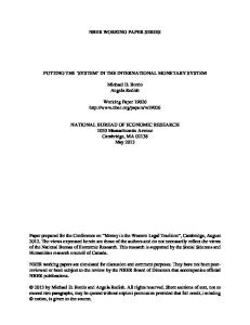
Fig. 4 Sample arrival states defined by �M and �M along the stable manifold.
0 �Xp0 ;
zf �
Necessary Conditions for Local Maxima
The optimization problem is converted to an unconstrained maximization formulation by adjoining all of the constraints (dynamical, control, and kinematic) to the performance index via Lagrange multipliers. This procedure is similar to previous approaches, but it is still custom to the problem at hand [11–13,40]. The multipliers $ and � are adjoined to the kinematic boundary conditions, the multiplier � is adjoined to the control constraints, and the costate vector � is adjoined to the dynamic constraints, resulting in the augmented performance index J0 :
(20)
t0
S
and ! represents the magnitude of the vector denoting the angular velocity of the rotating frame relative to the inertial frame. (Recall that in nondimensional units, I !S � 1.) Equations (16) and (17) use c and s as shorthand for sin and cos, respectively, and they represent a transformation from the Earth-centered inertial s^1 –s^2 –s^3 frame to the ^ y– ^ z^ frame. All computations are implemented rotating barycentric x– in this frame. For the powered phase, the spacecraft arrival point is at a state along the stable manifold associated with the periodic orbit. The stable manifold associated with the arrival orbit is generated a priori, and representative trajectories along the manifold are stored. Then, a two-dimensional cubic spline is used to approximate the states along the surface. Let the variables �M and �M represent free parameters that define a state along the stable manifold within the pregenerated data table. Recall Fig. 2, in which one trajectory along the manifold appears. The value of �M is an anglelike index associated with the fixed point X�ti � that determines where the manifold departs the periodic orbit; essentially, this variable identifies one representative trajectory along the surface. The maximum value of the associated �M counter corresponds to the total number of manifold trajectories that are generated around the entire periodic orbit. The value of �M is a timelike variable that is indexed to the backward propagation time along the stable manifold. Each manifold trajectory defined by �M is composed of a preselected total number of time element indices that are tagged by �M (see Fig. 4). Formulated with a fixed final time, the final kinematic boundary conditions f become position and velocity upon insertion at the match point; that is, � � r�tf � � rf ��M ; �M � (18) f �Xpf ; zf � � v�t � � v �� ; � � � 0 f f M M
B.
J0 � G�tf ; Xp0 ; Xpf ; z0 ; zf ; $; �� Zt f � L0 �t; Xp ; z; uc ; �; �� dt
� Tf �
@G � � �Tr @Xpf
�Tv
$Tv
k�
$m �
(33)
(34)
538
�
@G @z0
OZIMEK AND HOWELL
�T
2
3 � @rTpo ��; i; ��=@� @vTpo ��; i; ��=@� � �r0 T T 4 5 �0 � @rpo ��; i; ��=@i @vpo ��; i; ��=@i �v0 @rTpo ��; i; ��=@� @vTpo ��; i; ��=@� (35)
�
@G @zf
�T
� �
@rTM ��M ; �M �=@�M @rTM ��M ; �M �=@�M
@vTM ��M ; �M �=@�M @vTM ��M ; �M �=@�M
��
�rf �vf
� �0 (36)
Equations (25–27) are the costate equations and are of identical dimension (7 1) to the state equations. Equation (28) is trivial to the problem, but it is included due to the utilization of the parameters in the calculus of variations problem. Equations (29–32) are control optimality conditions and are used to partially formulate a control law. Finally, Eq. (29) implies that �v is parallel to u^ T ; thus, u^ T � �v =�v
(37)
where the normalization implicitly satisfies the first control constraint in Eq. (12). Equation (30) is solved directly to yield a parameterization for the thrust magnitude: T�
�v P �m m
(38)
Equations (12), (31), and (32) offer the following correlations for the engine power magnitude: 1) when cos � � 0, then P � Pmax ; 2) if sin � � 0, then P � 0; and, 3) if �2 � 0, then 0 P Pmax . Equations (33–35) are the transversality conditions and represent the equality constraints for the free optimization parameters. Only trivial values result from Eq. (33), but Eq. (34) demonstrates that the final value of the mass costate �mf must be the constant k, specified in Eq. (8). Because k is an arbitrary positive constant and �m always increases, due to Eq. (27), a degree of freedom is eliminated by scaling �m0 � 1. The first-order necessary conditions only guarantee a local extremal for Eq. (8), and a test for a local maximum is necessary to resolve the potential candidates for a control parameterization. Applying Pontryagin’s maximum principle [45] results in the following inequality condition: � Tv ��T =m�u^ T � � �m �T 2 =2P � � �Tv ��T=m�u^ T � � �m �T 2 =2P� (39) Of the two possibilities in Eq. (37), clearly Eq. (39) requires that u^ T � �v =�v
(40)
where the velocity costate vector �v now implies additional meaning as Lawden’s primer vector [46]. The observations 1–3 on the engine power P, resulting from Eqs. (31) and (32), are further reduced by substituting Eqs. (38) and (40) into Eq. (39); that is, �2 P �2v P � v 2 2 2� 2�m m mm
(41)
Because the first-order necessary conditions identify a value of �m that originates at one and always increases, Eq. (41) is always satisfied by defining P � Pmax . This choice automatically satisfies Eqs. (31) and (32) and the second constraint in Eq. (12) for the case when cos � is always zero. Thus, Eq. (38) becomes T�
�v Pmax �m m
The controls are now uniquely parameterized, and the TPBVP is completely defined. One of the most difficult aspects in obtaining a solution to an Euler–Lagrange formulation of the TPBVP is generating an accurate initial guess for the costate variables. As a result, _ , and _ are introduced to map the costates into the angles , , more physically realizable parameters using the ACT [18]. See Appendix A for further detail.
(42)
IV. Hybrid Direct/Indirect Solution Approach Both direct single shooting and direct multiple shooting are used to determine the low-thrust trajectories. These methods convert the functional optimization problem into a parameter optimization problem by a direct maximization on the performance index, rather than a root-solving process on all of the optimality constraint equations via an indirect approach. Thus, the hybrid term, as described by Gao and Kluever [22] and Kleuver and Pierson [23,24], reflects the fact that the calculus of variations TPBVP approach is used for the majority of the development (e.g., control parameterization via costates), but direct maximization replaces the indirect solving of (the often sensitive) transversality conditions. MATLAB’s® optimization toolbox function fmincon is used for the maximization. The gradient-based method used by fmincon for this study is a medium-scale sequential quadratic programming scheme with finite difference gradients. The function solves a quadratic programming (QP) subproblem at each iteration. An estimate of the Hessian of the Lagrangian is updated at each iteration with the Broyden–Fletcher–Goldfarb–Shanno formula. A line search is performed using a merit function, and the QP subproblem is solved using an active set strategy [47]. All integration is explicit and employs a Runge–Kutta–Verner 8(9) propagator, originally written in C and compiled in MATLAB via the MATLAB executable interface for speed. Further efficiency and accuracy will also be observed in the future by using analytical gradients. A.
Direct Single Shooting
Direct single shooting is useful in describing the problem with a relatively small number of design variables. For the direct single shooting approach, all of the unknown initial conditions and parameters (at each boundary) are selected as design variables. Thus, the design variable vector Sss is defined as S ss � f � i �
_ 0
_ 0
0
_ 0
T0
�_v
�M
� M gT (43)
The first nine design variables in Sss establish the state in the departure orbit, as well as the necessary information to predefine the entire state, costate, and control histories. Thus, the ACT is inherently incorporated, and the state and costates are explicitly propagated forward to tf , noting that the initial mass m0 is scaled, such that m0 � 1. The last two design variables specify the state at the match point on the invariant manifold. For implementation purposes, the parameter optimization objective function F is set equal to the negative final mass (the constant k is dropped here); that is, F�Sss � � �mf
(44)
The constraint vector, css �Sss � is equivalent to the terminal kinematic boundary conditions for the powered phase [Eq. (18)]. To aid in the convergence process, the cost function is not initially maximized, but a feasible solution satisfying css �Sss � is obtained. In this initial situation, the cost is set to minimize the least-squares error associated with the terminal constraints: F�Sss � � cTss �Sss �css �Sss �
(45)
Then, the complete NLP maximization process restarts with the feasible solution as an initial condition and Eq. (44) as the objective function. The function generator integrated into the NLP package for the process is summarized as follows:
539
OZIMEK AND HOWELL
Direct single shooting: Input: Sss Initialize: Xp via Eqs. (16) and (17) (scale m0 =1) and z Initialize: �0 via Eqs. (42) and (A1–A14) (�m0 � 1) Propagate: states [Eq. (9)] and costates [Eqs. (25–27)] using control laws of Eqs. (40) and (42) and P � Pmax from t � t0 to t � tf Terminate trajectory Compute objective and constraint: F�Sss � via Eq. (44) [or Eq. (45)] and css �Sss � via Eq. (18) B.
Direct Multiple Shooting
Direct multiple shooting is also used to compute low-thrust trajectories. Whereas the low number of design variables in single shooting methods is advantageous for simplicity, the same feature also means that the variables are susceptible to extreme sensitivity due to small changes propagating into very large nonlinear deviations downstream. This fact is especially true in the low-thrust problem, which is characterized by very long propagation times. Multiple shooting techniques are introduced to alleviate these precise difficulties in solving the TPBVP [9,19,20]. Let the time interval be decomposed into N segments: t0 < t1 < � � � < tN � tf
(46)
Note that the times for all interior nodes, t1 ; . . . ; tN�1 , are assumed to be fixed here. (TOF is still fixed, as defined previously.) Correspondingly, each interior node includes an unknown initial state and costate denoted by a � superscript that may be explicitly integrated forward: � � � X� p1 . . . XpN�1 ; �1 . . . �N�1
(47)
All of these unknown parameters become part of the new design variable vector: S ms � f STss
T
T
T
� X� P1 . . . XPN�1
T
� T �� 1 . . . �N�1 g
(48)
and the new constraint vector is ( c ms �
cs ccs css
) (49)
where cs and ccs are the state and costate constraints evaluated at the interior nodes, and css is the terminal constraint error that is also used in the direct single shooting approach. At an arbitrary interior node during time ti , the interior constraints are defined: c s �ti �X�pi � X� pi ;
ccs �ti � � ��i � �� i
(50)
The � superscript indicates that the state and costate are obtained at the termination of the direct integration of X� �ti�1 � and �� �ti�1 � over the time interval ti�1 to ti . If the length of the state vector is p (where p � 7, here), and the TOF at each interior node is fixed, then it is apparent that direct multiple shooting adds 2p �N � 2� design variables at the expense of 2p �N � 2� constraints. Similar to single shooting, the cost is evaluated as follows: F�Sms � � �mf
(51)
or F�Sms � � cTms �Sss �cms �Sss � where the feasible solution now includes the total error at each interior node. The advantage to the multiple shooting approach is that the individual design variable sensitivity is reduced, allowing for
more typically robust convergence, the freedom to add extra constraints to the nodes, and the possibility of parallel processing. The main disadvantage to the multiple shooting approach is the addition of function evaluations introduced by adding many new design variables and constraints (especially with finite difference gradients). Although not attempted here, some of this penalty may be offset by exploiting the sparsity of the Jacobian matrix [9]. In summary, the function generator for the multiple shooting approach is as follows: Direct multiple shooting Input: Sms Do for each segment i � 0, N � 1 if i � 0 Initialize: Xp0 via Eqs. (16) and (17) (scale m0 � 1) and z Initialize: �0 via Eqs. (42) and (A1–A14) (�m0 � 1) else � Initialize: X� pi , �i , ti , and ti�1 Propagate: states [Eq. (9)] and costates [Eqs. (25–27)] using control laws of Eq. (40) and (42) and P � Pmax from t � ti to t � ti�1 to obtain X�pi�1 , ��i�1 if i < N � 1 � Initialize: X� Pi�1 , �i�1 Compute interior node constraints: cs �ti�1 � and ccs �ti�1 � via Eq. (50) End Do Terminate trajectory Compute objective and final constraints: F�Sms � via Eq. (51) and css �Sms � via Eq. (18)
V.
Mission Scenario: Transfers To Lunar Coverage Orbits
One location of interest for future space exploration is the region near the lunar south pole. [5] From a range of orbits, various trajectories exposed in the CR3BP are potentially applicable in the mission design of lunar relay communication satellites for coverage of the south pole, due to the fixed geometry in the rotating frame and lineof-sight capability. For example, L1 and L2 southern halo orbits possess a line of sight with the lunar south pole over the majority of the orbital period and a line of sight with the Earth along the entire orbit. Thus, two spacecraft phased in such orbits yield continuous coverage of the lunar south pole. Additional orbital information on the periods and stability indices aids in the selection of specific orbits [5]. From the study by Grebow et al. [5], sample orbits are selected from the following families: L1 and L2 halo orbits, L1 and L2 vertical orbits, and L2 butterfly orbits [5] (see Fig. 5). Feasible transfer trajectories with a large convergence radius (i.e., with a high initial thrust magnitude) are easily determined from continuation procedures. Then, the initial thrust magnitude is iteratively lowered until the magnitude resembles a realistic value. For this study, the maximum allowable thrust is fixed at 1 N. As stated earlier, currently, this bound is not strictly imposed, but all solutions that violate this boundary are discarded or rerun. The assumed departure orbit and engine constants are listed in Table 1. Note that a large initial orbit radius of 20,000 km is employed. This initial condition is selected to quickly perform a preliminary proof-ofconcept study on many transfer scenarios with realistic thrust magnitudes. This approach is similar to other studies that use a realistic departure orbit radius but a thrust magnitude beyond current capabilities [24]. Departures from low-Earth orbit with realistic thrust magnitudes involve many spirals that consume significant computational expense and, at this time, are more suited to the design of an individual point solution during a more advanced design phase. Constraint tolerances for the match point are set to 1 10�10 nondimensional units on position and velocity. For consistency, each manifold tube is parameterized by the continuous variables �M � �1; . . . ; 50� and �M � �1; . . . ; 5000�. No restriction is placed upon the insertion location along the manifolds; however, all pregenerated data are propagated, such that a maximum of four Earth periapses are included. Direct single shooting is used in all examples to develop transfers. Direct multiple
540
OZIMEK AND HOWELL
Fig. 5 Potential periodic orbits for lunar south pole coverage.
shooting is employed in the first example (that is, transfer to a halo orbit), but because parallel processing is not involved and finite difference gradients are used, the increase in total function evaluations does not justify the decrease in the number of optimization iterations. Time history data are discussed for some of the halo orbit transfer examples, and the time history data for all other transfers are available in Appendix B. In general, transfer times are roughly 50–60% longer than the longest impulsive, ballistic lunar transfer times presented in a previous study by Perozzi and Di Salvo [48]. But, a sample transfer with realistic Isp yields a comparable TOF. A.
Four L1 Halo Orbit Transfers
Two 12-day L1 halo orbits with different z amplitudes are initially selected to demonstrate the construction of transfer trajectories. The orbit with the lower z amplitude (Az � 13; 200 km) is the focus of the first example 1) because it possesses the smaller out-of-plane excursion; and 2) because the manifolds retain their tubelike shape, thus the surface parameterization results in a smooth function for which the gradients of �M are well behaved with respect to the design variables. The resulting transfer appears in Fig. 6. It is plotted in both the Earth-centered rotating frame and the Earth-centered inertial frame. The black arcs along the trajectory indicate the powered phase, the blue asterisk represents the insertion point, and the coasting phase is green. The orbit color coincides with that in Fig. 5. In the inertial frame, the dotted line is the path of the moon. Typically, the locally optimizing procedure yields a small percentage increase from the feasible solutions with the fixed time-of-flight formulation. The oscillatory structure of the control histories are typical of all transfers, and an example appears in Fig. 7. (Tables 2 and 3 are also
Table 1 Departure orbit and engine constants Parameter
Value
Units
r0 m0 Pmax m l t Earth GM Moon GM Earth radius Moon radius
20,000 1500 10 6:04680403834987 1015 385,692.5 377,084.152667039 398,600.432896939 4902.80058214776 6378.14 1737.4
km kg kW kg km s km3 =s2 km3 =s2 km km
provided for a detailed list of the performance data for the optimal solutions.) The oscillation in the thrust magnitude to arrive at the manifold coasting state is a noted feature of the VSI engine in contrast to a traditional constant specific impulse engine, in which the behavior is operationally infeasible. In Fig. 7, the angle � represents the angular displacement of the thrust vector from the velocity vector. Thus, even though the thrust direction oscillates, it is closely aligned with the velocity vector during the initial spiral out and then shifts direction to meet the state at the match point. Both the in-plane ( ), and out-of-plane ( ) oscillations similarly reflect this behavior. The 182.8 day transfer is composed of 168.1 days of thrusting and 14.7 days of coasting along the manifold surface, yielding a delivery mass ratio of mf =m0 � 0:944. The trajectories along the stable manifold that are initially perturbed in the direction toward the moon may also be considered as targets for a transfer path. Such a transfer enables the possibility of a close lunar pass before insertion (see Fig. 8). From the two locally optimal solutions, no conclusions are drawn concerning the global behavior. From Fig. 6, it is apparent that the converged result relies on Isp ranges that are beyond the limitations of current technology when very low-thrust magnitudes are required. The results for this example (and other transfers investigated), however, yield insight for the insertion of coasting arcs to produce a comparable trajectory with current technology. To obtain Isp ranges that are an order of magnitude lower, the TOF associated with the transfer trajectory can be substantially lowered. Figures 9 and 10 represent a solution that remains below Isp � 3; 700 s for the duration of the powered arc. A more significant out-of-plane steering history for the angle is necessary to achieve insertion into the three-dimensional manifold path, given the reduced time, and the lower Isp levels lead to a comparatively lower delivery mass ratio of 0.881. The fourth example is a transfer to a 12-day L1 halo orbit, but the out-of-plane amplitude is now Az � 55; 700 km. To represent the manifold associated with this halo orbit, and for computational convenience, the manifold trajectories are spaced further apart than those for the previous 12-day orbit. Thus, the cubic spline approximation across �M degrades in comparison with the previous example. Whereas this degradation may be offset by increasing the density of the manifold trajectories (i.e., increasing the total range of integer values corresponding to �M ), the fixed demonstration value consistent with the previous example proves sufficient (see Fig. 11). A 155.5 day transfer is obtained, with 131.2 days of thrusting and coasting for 24.3 days. The slightly higher thrust values result in less overall conservation of mass propellant, as reflected in Table 2. The current formulation is primarily a thrusting portion, but in reality, the solution is a thrust arc followed by a coast arc.
541
OZIMEK AND HOWELL
Fig. 6
Low-thrust transfer to a 12-day, L1 halo orbit (Az � 13; 200 km) in rotating (left) and inertial (right) Earth-centered frames.
α (degrees)
T (mN)
600 400 200 0
50
100
50 0 −50
150
0
Powered Time (days) 1500
β (degrees)
m (kg)
1460 1440
0
50
60 40 20
100
150
0
Powered Time (days)
4
x 10
ζ (degrees)
4 2 0
50
100
50
100
150
Powered Time (days)
6
Isp (s)
150
0
1420
150
140 120 100 80 60 40 20 0
Powered Time (days)
B.
100
80
1480
Fig. 7
50
Powered Time (days)
50
100
150
Powered Time (days)
Time history data for low-thrust transfer to a 12-day L1 halo orbit (Az � 13; 200 km).
Transfers to L1 and L2 Vertical Orbits
The second class of orbits that are targeted for transfers are L1 and L2 vertical orbits. The L1 vertical orbit possesses an out-of-plane z amplitude Az � 57; 000 km. The associated stable manifold passes more than 150,000 km from Earth (that is, approximately 50,000 km further than any insertion point on the stable manifold corresponding to either of the two halo orbits). The manifolds are also significantly out of plane, but the shape of the tube is well preserved by the
trajectories, as in the sample transfer for the first 12-day halo orbit. The potential sensitivity to this out-of-plane behavior requires a departure orbit with a higher inclination (see Fig. 12 and Table 3). The transfer includes continuous thrusting for 138.0 and 31.2 days of coasting, for a total transfer time of 169.2 days. The next example is based on an L2 vertical orbit possessing a period of 16 days and Az � 57; 000 km. As �M varies during the pregeneration phase of the stable manifold, it is apparent that a
Table 2 Performance data for optimal solutions Orbit 12-day L1 12-day L1 12-day L1 12-day L1 14-day L1 16-day L2 14-day L2 a
mf =m0 halo 1 halo 1a halo 1b halo 2 vertical verticala butterfly
Lunar flyby Realistic Isp
b
0.944 0.940 0.881 0.927 0.935 0.935 0.937
Coast time, days Total time, days �V, km=s Tmin , mN Tmax , mN Tavg , mN 14.72 17.95 13.44 24.29 31.21 43.92 50.24
182.8 191.2 84.02 155.5 169.2 176.5 189.7
3.020 3.111 3.261 3.151 3.121 3.158 3.178
28.20 27.27 551.2 105.2 169.2 175.8 106.8
673.4 765.1 999.4 816.8 723.3 601.9 634.6
230.0 208.0 722.9 321.2 309.0 363.1 364.8
542
OZIMEK AND HOWELL
Table 3 12-day
Converged design variable values for orbit examples 12-day
12-day a
12-day
16-day
14-day
L1 halo 2
L1 vertical
L2 vertical
�132:492 20.7338 181.936 3.02533 8.36250 6.10449 �25:4581 692.017 4.43903 45.0002 3079.45
70.2552 10.9948 192.559 0.598876 5.65886 �3:09303 �30:8696 651.567 1.31372 17.2723 3501.65
41.4733 11.5811 225.080 3.01643 �4:92376 �2:28378 �1:01189 565.892 4.13983 6.00000 4214.50
Parameter
L1 halo 1
L1 halo 1
L1 halo 1
�, deg i, deg �, deg 0 , 10�2 rad _ 0 ( 10�6 rad=s)
0 , 10�2 rad
_ 0 , 10�7 rad=s T0 , mN �_v0 , 10�1 �M �M
227.972 4.43307 209.378 �2:06274 8.64493 2.99752 �37:6027 579.096 �1:93538 16.7476 2423.11
115.534 �8:85154 311.789 �1:76465 �2:36955 1.57578 �3:45285 742.297 �2:99295 1.00000 2739.55
111.090 15.608 158.397 1.78903 1.75023 24.0023 �1:04283 765.501 2.40023 2.00006 2075.28
a
14-day
b
a
L2 butterfly 22.3892 22.1900 210.020 �4:60049 9.46877 7.41943 �58:0872 404.598 �1:40822 1.00000 4401.13
Lunar flyby Realistic Isp
b
smooth tubular structure is not a good mathematical assumption for this manifold. The lack of a well-defined surface impacts the gradients corresponding to the cost and constraints with respect to �M ; therefore, the variable is completely removed from the problem by fixing a trajectory of interest (i.e., fixing �M ). Despite the elimination of a design variable, a solution is still obtained, yet it is only a local minimum for a single trajectory associated with the fixed point. It is also apparent in Fig. 13 that the converged trajectory
exhibits a close passage of the moon to reach the translunar periodic orbit. The resulting 176.4 day transfer includes 132.5 days of thrusting and a 44.0 day coast. C.
Transfer to an L2 Butterfly Orbit
The final orbit from Fig. 5 for demonstration of the design of lowthrust transfers in this problem is a 14-day L2 butterfly orbit. The
Fig. 8 Low-thrust transfer to a 12-day L1 halo orbit (Az � 13; 200 km) using a lunar flyby in rotating (left) and inertial (right) Earth-centered frames.
Fig. 9 Low-thrust transfer to a 12-day L1 halo orbit (Az � 13; 200 km) with realistic specific impulse ranges in rotating (left) and inertial (right) Earthcentered frames.
543
OZIMEK AND HOWELL
α (degrees)
T (mN)
900 800 700
5 0 −5
600 0
20
40
60
0
20
40
60
Powered Time (days)
1500
60
1450
40
β (degrees)
m (kg)
Powered Time (days)
1400 1350
20 0 −20
0
20
40
60
0
Powered Time (days)
20
40
60
Powered Time (days) 60
ζ (degrees)
Isp (s)
3500 3000 2500
0
20
40
Powered Time (days)
60
40 20
0
20
40
60
Powered Time (days)
Fig. 10 Time history data for low-thrust transfer to a 12-day L1 halo orbit (Az � 13; 200 km) with realistic specific impulse ranges.
Fig. 11
Low-thrust transfer to a 12-day L1 halo orbit (Az � 55; 700 km) in rotating (left) and inertial (right) Earth-centered frames.
Fig. 12
Low-thrust transfer to a 14-day L1 vertical orbit in rotating (left) and inertial (right) Earth-centered frames.
544
OZIMEK AND HOWELL
Fig. 13
Low-thrust transfer to a 16-day L2 vertical orbit in rotating (left) and inertial (right) Earth-centered frames.
Fig. 14 Low-thrust transfer to a 14-day L2 butterfly orbit in rotating (left) and inertial (right) Earth-centered frames.
initially targeted insertion state along the stable manifold, similar to the sample transfers to the vertical orbits, is over 150,000 km (actually 162,000 km) from Earth. Again, similar to the 16-day L2 vertical orbit, a smooth surface is not formed when �M is varied during the initial manifold generation. This behavior is actually observed in several L2 orbits, due to the often large regions of exclusion that can prevent individual manifold trajectories from passing within the vicinity of the Earth. As a result, the anglelike parameter �M is again fixed. The near stability of this orbit also correlates to a longer coasting time along the manifold trajectory, as noted in Table 2. The final converged trajectory appears in Fig. 14.
VI.
Conclusions
The restricted three-body problem is used to construct preliminary designs for low-thrust transfers to libration point orbits. These transfers are based on the existence of predefined reference coast arcs computed as trajectories on invariant manifolds associated with the periodic orbit. Primer vector theory yields a control law that is parameterized in terms of costate variables for a VSI engine model. Additional optimality constraints also prove to be useful in establishing the design variables (via the ACT). The well-known ACT allows the specification of costates without an a priori value. NLP with explicit numerical integration via direct single shooting and direct multiple shooting is used as a basis to obtain transfers that locally maximize the final spacecraft mass. This approach can be
successfully employed to demonstrate an initial proof of concept involving a mission scenario that uses Earth–moon libration point orbits for potential lunar south pole coverage. Feasible transfers are systematically generated with a continuation method that iteratively lowers the initial thrust value until the problem constraints are satisfied. Maximization via NLP then results in increased final mass delivery with respect to the feasible solution with the same TOF. The departure orbit under consideration may also be slightly modified to include more general classes of conics defined by an initial set of complete orbital elements. Such initial conditions may be useful, for example, if a spacecraft is placed into a geosynchronous transfer orbit (GTO). An example of a low-thrust transfer from GTO to a 12-day L1 halo orbit (Az � 13; 200 km) appears in Figs. B6 and B7. Ongoing work will rigorously consider the type of departure orbit within the context of the potential mission application. These ongoing efforts also involve the generation of initial conditions that meet realistic thrust and Isp ranges, exploiting the advantages of a system model in spherical coordinates [12], and high fidelity modeling.
Appendix A: Adjoint Control Transformation Consider a reference frame centered at the spacecraft and defined by the unit vectors v^ � w^ � h^ (i.e., the vwh frame). The v^ axis is aligned with the velocity vector v. The h^ axis is parallel to the instantaneous angular momentum vector r v. Finally, the w^ axis is
545
OZIMEK AND HOWELL
2
defined to complete a right-handed system. These unit vectors, and the associated time derivatives, are defined as r v h^ � ; kr vk
v v^ � ; v
w^ � h^ v^
(A1)
2
_^ i^ � v_^ i^ � w 6^ _ ^ _ _ R � 4 j � v^ j � w^ _^ k^ � v_^ k^ � w
3 _ i^ � h^ _7 j^ � h^ 5 _ k^ � h^
_ � vv=v _ 2 v_^ � v=v
(A2)
u^ Tijk � Ru^ Tvwh
(A10)
_ _ � hh=h _ 2 h^ � h=h
(A3)
_ u^ T � Ru_^ T u_^ Tijk � R vwh vwh
(A11)
_^ � h_^ v^ � h^ v_^ w
(A4)
_ v_ � v � v=v _ h_ � h � h=h
sin cos sin �T
u^ Tvwh � � cos cos
3 � _ sin cos � _ cos sin
� 4 _ cos cos � _ sin sin 5
_ cos
� v � �v u^ Tijk
(A6)
where �v is the magnitude of the primer vector �v � k�v k. Then, the equation of motion for the primer vector, Eq. (26), is directly involved in parameterizing the position costate vector: @h�v� � r � ��_ v � �Tv @v
(A8)
Because the equations of motion are integrated in the Cartesian ^ a rotation barycentric rotating frame (with unit vectors i^ � j^ � k), matrix R is required to transform the thrust direction, u^ Tvwh (and u_^ Tvwh ):
�_ v � ��_v u^ Tijk � �v u_^ Tijk
400 200 0
50
100
Time history data are generated for the remaining orbit examples, and detailed in Figs. B1–B5. An example transfer considering a departure from GTO appears in Figs. B6 and B7.
50 0 −50
150
0
1500
β (degrees)
m (kg)
100
150
0
1440 1420
−20 −40 −60 −80
0
50 4
x 10
100
150
0
Powered Time (days)
50
100
150
Powered Time (days) 100
ζ (degrees)
6
Isp (s)
50
Powered Time (days)
1460
4 2 0
50
100
Powered Time (days)
150
(A14)
Appendix B: Additional Low-Thrust Transfer Results
Powered Time (days) 1480
(A13)
Additionally, Eq. (42) is used to parameterize �v in terms of the thrust T. Thus, the mapping sequence allows �r and �v to be calculated _ T, and �_v . _ , , from , ,
α (degrees)
600
(A12)
The derivative of the primer vector �_ v is also available by differentiating Eq. (A12) and substituting the result into Eq. (A13):
(A7)
2
T (mN)
The subscript ijk denotes that the thrust direction is expressed in terms of unit vectors in the barycentric rotating frame. The definition of the thrust direction from Eq. (40) is employed to parameterize the primer vector:
(A5)
Two spherical angles, and , as well as their time derivatives, _ and _ specify the orientation of the thrust direction relative to this frame,
, u^ Tvwh , and also the time derivative of the thrust direction, u_^ Tvwh ; that is,
Fig. B1
3 i^ � h^ j^ � h^ 5; k^ � h^
(A9)
Given a vector and its time derivative, the following relationships are also exploited to fully determine Eqs. (A2–A4):
u_^ Tvwh
i^ � v^ i^ � w^ R � 4 j^ � v^ j^ � w^ k^ � v^ k^ � w^
80 60 40 20 0
50
100
150
Powered Time (days)
Time history data for low-thrust transfer to a 12-day l1 halo orbit (aZ � 13; 200 km) using a lunar flyby.
546
OZIMEK AND HOWELL
α (degrees)
800
T (mN)
600 400 200 0
50
50 0 −50
100
0
Powered Time (days)
50
100
Powered Time (days)
β (degrees)
m (kg)
1500
1450
1400
0 −50
0
50 4
100
0
Powered Time (days)
1.5 1 0.5 0
50
100
100
120 100 80 60 40 20 0
Powered Time (days)
50
100
Powered Time (days)
Time history data for low-thrust transfer to a 12-day l1 halo orbit (aZ � 55; 700 km).
Fig. B2
α (degrees)
600
T (mN)
50
Powered Time (days)
ζ (degrees)
x 10
Isp (s)
50
400 200 0
50
5 0 −5
100
0
Powered Time (days)
50
100
Powered Time (days)
1500
β (degrees)
m (kg)
1480 1460 1440 1420
−10 −20
0
50 4
100
0
Powered Time (days)
1.5 1 0.5 0
50
100
Powered Time (days)
Fig. B3
50
100
Powered Time (days)
ζ (degrees)
x 10
Isp (s)
0
20 15 10 5 0
50
100
Powered Time (days)
Time history data for low-thrust transfer to a 14-day l1 vertical orbit.
547
OZIMEK AND HOWELL
α (degrees)
600
T (mN)
500 400 300
5 0 −5
200 0
50
100
0
Powered Time (days) 1500
100
30
β (degrees)
1480
m (kg)
50
Powered Time (days)
1460 1440 1420 0
50
20 10 0
100
0
Powered Time (days)
50
100
Powered Time (days) 30
ζ (degrees)
Isp (s)
10000 8000 6000
20 10
4000 0
50
100
0
Powered Time (days)
Fig. B4
α (degrees)
10
500
T (mN)
100
Time history data for low-thrust transfer to a 16-day l2 vertical orbit.
600
400 300 200
5 0 −5 −10
0
50
100
0
Powered Time (days)
50
100
Powered Time (days)
1500
40
β (degrees)
1480
m (kg)
50
Powered Time (days)
1460 1440
20 0
1420 0
50 4
x 10
100
0
Powered Time (days)
50
100
Powered Time (days)
ζ (degrees)
40
Isp (s)
1.5 1
30 20 10
0.5 0
50
100
Powered Time (days)
0
50
100
Powered Time (days)
Fig. B5 Time history data for low-thrust transfer to a 14-day l2 butterfly orbit.
548
OZIMEK AND HOWELL
Fig. B6
Low-thrust transfer to a 12-day l1 halo orbit (aZ � 13; 200 km) via a GTO departure condition.
50
α (degrees)
T (mN)
800 600 400 200
0
−50 0
20
40
60
0
Powered Time (days)
20
40
60
Powered Time (days)
β (degrees)
m (kg)
1500 1480 1460
0 −20 −40
1440 0
20 4
x 10
40
60
ζ (degrees)
Isp (s)
4 2 0
20
40
20
40
60
Powered Time (days)
6
60
Powered Time (days)
Fig. B7
0
Powered Time (days) 60 40 20 0
20
40
60
Powered Time (days)
Time history data for low-thrust transfer to a 12-day l1 halo orbit (Az � 13; 200 km) via a GTO departure condition.
Acknowledgments The work was supported by Purdue University under the Andrews Fellowship and by NASA under contract number NNX06AC22G. A portion of this work was completed at the NASA Goddard Space Flight Center under the supervision of David Folta.
References [1] Farquhar, R., “Mission Design for a Halo Orbiter of the Earth,” Journal of Spacecraft and Rockets, Vol. 14, No. 3, March 1977, pp. 170–177. doi:10.2514/3.57176 [2] Farquhar, R., “The Utilization of Halo Orbits in Advanced Lunar Operations,” NASA TN D-6365, Goddard Spaceflight Center, Greenbelt, MD, 1971. [3] Ely, T., “Stable Constellations of Frozen Elliptical Inclined Orbits,” Journal of the Astronautical Sciences, Vol. 53, No. 3, July–Sept. 2005, pp. 301–316. [4] Ely, T., and Lieb, E., “Constellations of Elliptical Inclined Lunar Orbits Providing Polar and Global Coverage,” Journal of the Astronautical
Sciences, Vol. 54, No. 1, 2007, pp. 1447–1463. [5] Grebow, D., Ozimek, M., Howell, K., and Folta, D., “Multi-Body Orbit Architectures for Lunar South Pole Coverage,” Journal of Spacecraft and Rockets, Vol. 45, No. 2, 2008, pp. 344–358. doi:10.2514/1.28738 [6] Howell, K., Grebow, D., and Olikara, Z., “Design Using Gauss’ Perturbing Equations With Applications to Lunar South Pole Coverage,” Proceedings of the AAS/AIAA Space Flight Mechanics Meeting, Advances in the Astronautical Sciences, Vol. 127, No. 1, Univelt, San Diego, CA, 2007, pp. 641–670; also AAS Paper 07-143. [7] Rayman, M., Varghese, P., Lehman, D., and Livesay, L., “Design of the First Interplanetary Solar Electric Propulsion Mission,” Journal of Spacecraft and Rockets, Vol. 39, No. 4, August 2002, pp. 589–595. doi:10.2514/2.3848 [8] Schoenmaekers, J., Horas, D., and Pulido, J., “SMART-1: With Solar Electric Propulsion to the Moon,” Proceedings of the 16th International Symposium on Space Flight Dynamics, NASA Jet Propulsion Lab., Pasadena, CA, 2001, p. 114. [9] Betts, J., “Survey of Numerical Methods for Trajectory Optimization,” Journal of Guidance, Control, and Dynamics, Vol. 21, No. 2, March–
OZIMEK AND HOWELL
[10] [11]
[12]
[13]
[14] [15] [16]
[17]
[18]
[19] [20] [21]
[22]
[23]
[24]
[25]
[26]
[27]
[28]
[29]
April 1998, pp. 193–207. doi:10.2514/2.4231 Hull, D., Optimal Control Theory for Applications, Springer, New York, 2003, pp. 247–255, 350–365. Ranieri, C., and Ocampo, C., “Optimization of Roundtrip, TimeConstrained, Finite Burn Trajectories via an Indirect Method,” Journal of Guidance, Control, and Dynamics, Vol. 28, No. 2, March– April 2005, pp. 306–314. doi:10.2514/1.5540 Ranieri, C., and Ocampo, C., “Indirect Optimization of Spiral Trajectories,” Journal of Guidance, Control, and Dynamics, Vol. 29, No. 6, Nov.–Dec. 2006, pp. 1360–1366. doi:10.2514/1.19539 Russell, R., “Primer Vector Theory Applied to Global Low-Thrust Trade Studies,” Journal of Guidance, Control, and Dynamics, Vol. 30, No. 2, March–April 2007, pp. 460–473. doi:10.2514/1.22984 Edelbaum, T., “Optimum Power-Limited Orbit Transfer in Strong Gravity Fields,” AIAA Journal, Vol. 3, No. 5, May 1965, pp. 921–925. doi:10.2514/3.3016 Melbourne, W., “Three-Dimensional Optimum Thrust Trajectories,” NASA JPL-TR-32-98, Pasadena, CA, 1961. Melbourne, W., and Sauer, C., “Optimum Interplanetary Rendezvous with Power-Limited Vehicles,” AIAA Journal, Vol. 1, No. 1, Jan. 1963, pp. 54–60. doi:10.2514/3.1468 Redding, D., and Breakwell, J., “Optimal Low-Thrust Transfers to Synchronous Orbit,” Journal of Guidance, Control, and Dynamics, Vol. 7, No. 2, March–April 1984, pp. 148–155. doi:10.2514/3.8560 Dixon, L., and Biggs, M., “Adjoint-Control Transformations for Solving Practical Optimal Control Problems,” Optimal Control Applications and Methods, Vol. 2, No. 4, 2007, pp. 365–381. doi:10.1002/oca.4660020405 Stoer, J., and Bulirsch, R., Introduction to Numerical Analysis, Springer–Verlag, New York, 1980. Keller, H., Numerical Methods for Two-Point Boundary Value Problems, Blaisdell, London, 1968, pp. 13–14. Vadali, S., and Nah, R., “Fuel-Optimal Planar Earth-Mars Trajectories Using Low-Thrust Exhaust-Modulated Propulsion,” Journal of Guidance, Control, and Dynamics, Vol. 23, No. 3, May–June 2000, pp. 476–482. doi:10.2514/2.4553 Gao, Y., and Kluever, C., “Low-Thrust Interplanetary Orbit Transfers Using Hybrid Trajectory Optimization Method with Multiple Shooting,” AIAA/AAS Astrodynamics Specialist Conference and Exhibit, AIAA Paper 2004-4088, Aug. 2004. Pierson, B., and Kluever, C., “Three-Stage Approach to Optimal LowThrust Earth–Moon Trajectories,” Journal of Guidance, Control, and Dynamics, Vol. 17, No. 6, Nov.–Dec. 1994, pp. 1275–1282. doi:10.2514/3.21344 Kluever, C., and Pierson, B., “Optimal Low-Thrust Three-Dimensional Earth–Moon Trajectories,” Journal of Guidance, Control, and Dynamics, Vol. 18, No. 4, July–Aug. 1995, pp. 830–837. doi:10.2514/3.21466 Petropoulos, A., and Russell, R., “Low-Thrust Transfers Using Primer Vector Theory and a Second-Order Penalty Method,” AAS/AIAA Astrodynamics Specialist Conference and Exhibit, AIAA Paper 20086955, 18–21 Aug. 2008. Hargraves, C., and Paris, S., “Direct Trajectory Optimization Using Nonlinear Programming and Collocations,” Journal of Guidance, Control, and Dynamics, Vol. 10, No. 4, July–Aug. 1987, pp. 338–342. doi:10.2514/3.20223 Enright, P., and Conway, B., “Discrete Approximations to Optimal Trajectories Using Direct Transcription and Nonlinear Programming,” Journal of Guidance, Control, and Dynamics, Vol. 15, No. 4, July– Aug. 1992, pp. 994–1002. doi:10.2514/3.20934 Herman, A., and Conway, B., “Optimal, Low-Thrust, Earth–Moon Orbit Transfer,” Journal of Guidance, Control, and Dynamics, Vol. 21, No. 1, Jan.–Feb. 1998, pp. 141–147. doi:10.2514/2.4210 Betts, J., and Erb, S., “Optimal Low Thrust Trajectories to the Moon,” SIAM Journal on Applied Dynamical Systems, Vol. 2, No. 2, 2003, pp. 144–170. doi:10.1137/S1111111102409080
549
[30] Conway, B., and Larson, K., “Collocation Versus Differential Inclusion in Direct Optimization,” Journal of Guidance, Control, and Dynamics, Vol. 21, No. 5, Sept.–Oct. 1998, pp. 780–785. doi:10.2514/2.4306 [31] Hargens, J., and Coverstone, V., “Low-Thrust Interplanetary Mission Design Using Differential Inclusion,” AIAA/AAS Astrodynamics Specialist Conference and Exhibit, AIAA Paper 2002-4730, Aug. 2002. [32] Whiffen, G., and Sims, J., “Application of the SDC Optimal Control Algorithm to Low-Thrust Escape and Capture Trajectory Optimization,” AAS/AIAA Space Flight Mechanics Meeting, Advances in the Astronautical Sciences, Vol. 112, No. 1, Univelt, San Diego, CA, 2002, pp. 1361–1383; also American Astronautical Society Paper 02-208. [33] Hartmann, J., Coverstone-Carroll, V., and Williams, S., “Optimal Interplanetary Spacecraft Trajectories via a Pareto Genetic Algorithm,” Journal of the Astronautical Sciences, Vol. 46, No. 3, 1998, pp. 267– 282. [34] Vavrina, M., and Howell, K., “Multiobjective Optimization of LowThrust Trajectories Using a Genetic Algorithm,” AAS/AIAA Space Flight Mechanics Meeting, American Astronautical Society Paper 09151, Savannah, GA, Feb. 2009. [35] Gómez, G., Jorba, A., and Masdemont, J., “Study of the Transfer from the Earth to a Halo Orbit Around the Equilibrium Point L1 ,” Celestial Mechanics and Dynamical Astronomy, Vol. 56, No. 4, Aug. 1993, pp. 541–562. doi:10.1007/BF00696185 [36] Howell, K., Mains, D., and Barden, B., “Transfer Trajectories From Earth Parking Orbits to Sun–Earth Halo Orbits,” AAS/AIAA Space Flight Mechanics Meeting, Advances in the Astronautical Sciences, Vol. 87, No. 1, Univelt, San Diego, CA, 1994, pp. 399–422; also American Astronautical Society Paper 94-160. [37] Starchville, T., and Melton, R., “Optimal Low-Thrust Trajectories to Earth–Moon L2 Halo Orbits (Circular Problem),” AAS/AIAA Astrodynamics Specialist Conference, Advances in the Astronautical Sciences, Vol. 97, No. 1, Univelt, San Diego, CA, 1997, pp. 1741–1757; also American Astronautical Society Paper 97-714. [38] Starchville, T., and Melton, R., “Optimal Low-Thrust Transfers to Halo Orbits about the L2 Libration Point in the Earth–moon System (Elliptical Problem),” AAS/AIAA Space Flight Mechanics Meeting, Advances in the Astronautical Sciences, Vol. 99, No. 1, Univelt, San Diego, CA, 1998, pp. 1489–1506; also American Astronautical Society Paper 98-205. [39] Sukhanov, A., and Eismont, N., “Low Thrust Transfer to Sun–Earth L1 and L2 Points with a Constraint on the Thrust Direction,” Proceedings of the Libration Point Orbits and Applications Conference, World Scientific, London, 2003, pp. 439–454. [40] Senent, J., Ocampo, C., and Capella, A., “Low-Thrust VariableSpecific-Impulse Transfers and Guidance to Unstable Periodic Orbits,” Journal of Guidance, Control, and Dynamics, Vol. 28, No. 2, March– April 2005, pp. 280–290. doi:10.2514/1.6398 [41] Mingotti, G., Topputo, F., and Bernelli-Zazzera, F., “Combined Optimal Low-Thrust and Stable-Manifold Trajectories to the Earth– Moon Halo Orbits,” New Trends in Astrodynamics and Applications 3, Vol. 886, Feb. 2007, pp. 100–112. doi:10.1063/1.2710047 [42] Russell, R., and Lam, T., “Designing Ephemeris Capture Trajectories at Europa using Unstable Periodic Orbits,” Journal of Guidance, Control, and Dynamics, Vol. 30, No. 2, March–April 2007, pp. 482–491. doi:10.2514/1.22985 [43] Poincaré, H., New Methods of Celestial Mechanics, edited by D. Goroff, Springer, New York, 2007. [44] Perko, L., Differential Equations and Dynamical Systems, Springer– Verlag, New York, 1991, pp. 220–234. [45] Pontryagin, L., The Mathematical Theory of Optimal Processes, Interscience, New York, 1962, pp. 9–108. [46] Lawden, D., Optimal Trajectories for Space Navigation, Butterworths, London, 1963, pp. 54–126. [47] Gill, P., Murray, W., Saunders, M., and Wright, M., “Procedures for Optimization Problems with a Mixture of Bounds and General Linear Constraints,” ACM Transactions on Mathematical Software, Vol. 10, No. 3, Sept. 1984, pp. 282–298. doi:10.1145/1271.1276 [48] Perozzi, E., and Di Salvo, A., “Novel Spaceways for Reaching the Moon: An Assessment for Exploration,” Celestial Mechanics and Dynamical Astronomy, Vol. 102, Nos. 1–3, Sept. 2008, pp. 207–218. doi:10.1007/s10569-008-9156-3