Monetary Policy and Sovereign Debt Sustainability Galo Nuño

Carlos Thomas

Banco de España

Banco de España

First version: March 2015 This version: July 2016

Abstract We investigate the welfare consequences of optimal discretionary monetary policy, in a small open economy model where the government issues nominal debt without committing not to default or in‡ate. In‡ation absorbs the e¤ect of aggregate shocks on the debt ratio, making (costly) defaults less likely ex ante. But the government incurs an ‘in‡ationary bias’: it creates (costly) in‡ation even when default is distant. For plausible calibrations, we …nd that abandoning the ability to in‡ate debt away raises welfare, even when the economy is close to default: the bene…ts from eliminating the in‡ationary bias dominate the costs from losing in‡ation’s debt-stabilizing role. Keyword s: monetary and …scal policy, discretion, sovereign default, state-contingent in‡ation, in‡ationary bias, continuous time, optimal stopping. JEL codes: E5, E62,F34 The views expressed in this paper are those of the authors and do not necessarily represent the views of Banco de España or the Eurosystem. This manuscript was previously circulated as "Monetary Policy and Sovereign Debt Vulnerability". The authors are very grateful to Fernando Álvarez, Manuel Amador, Óscar Arce, Cristina Arellano, Javier Bianchi, Antoine Camous, Giancarlo Corsetti, Jose A. Cuenca, Luca Dedola, Antonia Diaz, Aitor Erce, Maurizio Falcone, Esther Gordo, Jonathan Heathcote, Alfredo Ibañez, Fabio Kanczuk, Peter Karadi, Matthias Kredler, Xiaowen Lei, Albert Marcet, Benjamin Moll, Juan P. Nicolini, Ricardo Reis, Juan P. Rincón-Zapatero, Pedro Teles, conference participants at the SED Annual Meeting, REDg Workshop, Oxford-FRB of New York Monetary Economics Conference, Barcelona GSE Summer Forum, Banco do Brasil Annual In‡ation Targeting Seminar, Theories and Methods in Macroeconomics Conference, European Winter Meetings of the Econometric Society, and seminar participants at Université Paris-Dauphine, Universidad Carlos III, FRB of Minneapolis, ECB, Banca d’Italia, BBVA, Banco de España, European Commission, Universidad de Vigo, and University of Porto for helpful comments and suggestions. All remaining errors are ours.

1

1

Introduction

One of the main legacies of the 2007-9 …nancial crisis and the subsequent recession has been the emergence of large …scal de…cits across the industrialized world, resulting in government debtto-GDP ratios near or above record levels in countries such as the United States, the United Kingdom, or the Euro area periphery. Before the summer of 2012, the peripheral Euro area economies experienced dramatic spikes in their sovereign default premia, whereas other highly indebted countries such as the US and the UK did not. Many observers emphasized that a key di¤erence between both groups of countries was that, whereas the US and the UK controlled the supply of the currency in which they issued their debt and hence had the option to reduce its real value by creating in‡ation, such an option was not available to the peripheral Euro area economies. In recent years, sovereign debt troubles have lingered on (and at times intensi…ed) in countries such as Greece, with many voices asking again whether those countries would have been better o¤ with an independent monetary policy. These developments raise the question as to whether or not an economy may bene…t from retaining the ability to stabilize its debt by in‡ating it away. In this paper, we try to shed light on the above question by studying the welfare implications of in‡ation when the government cannot commit not to default explicitly on its debt, but also not to reduce its real value through in‡ation. With this purpose, we build a general equilibrium, continuous-time model of a small open economy in which a benevolent government issues longterm noncontingent nominal bonds to foreign investors. As in standard quantitative models of optimal sovereign default (e.g. Aguiar and Gopinath 2006, and Arellano 2008), the government may default at any time and thus reduce its debt burden, but at the expense of temporary exclusion from capital markets (thus losing the ability to smooth consumption) and a drop in the output endowment. The default decision is characterized by an optimal default threshold for the model’s single state variable, the debt-to-GDP ratio. In addition, the government chooses optimal …scal and monetary policy under discretion, i.e. without commitments on the future path of primary de…cits and in‡ation. In‡ation reduces the real value of debt ceteris paribus, but also entails welfare costs due to costly price adjustment. The optimal monetary policy features an ‘in‡ationary bias’: the government chooses positive in‡ation as long as outstanding debt is positive. We refer to this baseline scenario as the ’in‡ationary regime’. As explained above, our focus is on the welfare consequences of being able to in‡ate away the debt under discretion. With this purpose, we compare the baseline in‡ationary regime with a scenario in which in‡ation is zero at all times. This ’no in‡ation’ regime can be interpreted as a situation in which the country joins a monetary union with a very strong and credible antiin‡ationary stance, thus losing its ability to in‡ate its debt away; or alternatively, as a situation in which the government issues foreign currency debt, such that there is no bene…t from creating

2

in‡ation. We calibrate our model to capture some salient features of the euro area peripheral economies, such as the volatility of their aggregate ‡uctuations and their in‡ation record prior to joining the euro. We show that, in the in‡ationary regime, optimal in‡ation increases monotonically with the debt ratio; this increase is nearly linear for most debt ratios, and becomes very steep as the economy approaches the default threshold. Our main result is that, for our baseline calibration, welfare in the no-in‡ation regime is higher at any debt ratio, even close to the default threshold.1 That is, the economy considered here does not bene…t from retaining the ability to in‡ate away its debt at discretion, regardless of how far or imminent sovereign default may be. This result re‡ects the di¤erent bene…ts and costs of optimal discretionary in‡ation in this framework. Let us begin with the bene…ts. Because debt is nominal and noncontingent, unanticipated in‡ation makes ex-post real returns state-contingent. This allows the government to partially absorb the impact of aggregate shocks on the debt ratio and thus improve consumption smoothing. The welfare bene…ts of state-contingent in‡ation in models that abstract from default are well known.2 The novelty here is that, when the government cannot commit to repay, the shock-absorbing role of state-contingent in‡ation becomes even more valuable, because it makes default a less likely outcome ex ante. In response to negative output shocks that raise the debt ratio and hence bring it closer to the default threshold, the government creates positive in‡ation surprises that partially undo the impact of the shock on the debt ratio. This way, in‡ation delays ex ante the arrival of sovereign default and the ensuing autarky period, where social welfare is at its lowest due to the aforementioned default costs. We now turn to the costs of discretionary optimal in‡ation. As mentioned before, the in‡ationary regime su¤ers from an in‡ationary bias by which the government cannot avoid the temptation to create in‡ation even at relatively low debt ratios, for which default is still perceived is rather distant. This in turn entails two kinds of costs. The …rst are the direct utility costs of (contemporaneous) in‡ation mentioned before. The second stems from expectations of future in‡ation during the life of the bond, which depress nominal bond prices (equivalently, raise nominal bond yields) vis-à-vis the no in‡ation regime. Lower nominal bond prices make primary de…cits more costly to …nance, leading the government to reduce consumption for given exogenous output. Moreover, higher nominal yields undo much of the bene…cial e¤ect of in‡ation on ex-post real bond returns, thus impairing debt stabilization. Which of these e¤ects dominate is a quantitative question. For our euro area calibration, the welfare costs from the in‡ationary bias dominate the bene…ts of state-contingent in‡ation, including the improvement in sovereign debt sustainability.3 Interestingly, the welfare gap narrows 1

Interestingly, we also …nd that optimal default thresholds are nearly identical in both regimes, such that they both share essentially the same equilibrium no-default region. 2 See the discussion of the related literature at the end of this section. 3 This is manifested in equilibrium bond yields, which are higher in the in‡ationary regime at all debt ratios,

3

as both economies approach their respective default thresholds. This re‡ects the fact that, as the economy gets closer to default, the debt-stabilizing role of in‡ation becomes more and more valuable. In fact, for debt ratios su¢ ciently close to default, the in‡ationary regime achieves a higher expected stream of consumption utility ‡ows. However, this bene…t is never large enough to compensate for the expected stream of in‡ation disutility costs from the in‡ationary bias.4 We show that our …ndings are robust to a wide range of alternative parameter values, including those controlling in‡ation and default costs. We also …nd that, if ‡uctuations in output growth are large enough, then for debt ratios su¢ ciently close to default the in‡ationary regime may outperform the no-in‡ation one, for it is then that the bene…cial e¤ects of state-contingent in‡ation as a debt-stabilizing tool outweigh the costs from the in‡ationary bias. However, the necessary level of output growth volatility is too high to be of much practical importance. We conclude that, for empirically plausible calibrations, our main results on the desirability of relinquishing discretionary in‡ation policies remain robust.5 Taken together, our results o¤er an important quali…cation of the conventional wisdom that individual countries may bene…t from retaining the option to in‡ate away their sovereign debt. In particular, our analysis suggests that such countries may actually be better o¤ by renouncing such a tool if their governments are unable to make credible commitments about their future in‡ation policy. Our …ndings may also rationalize why a number of developing countries with limited in‡ation credibility typically resort to issuing debt in terms of a hard foreign currency. Related Literature. Our paper relates to several strands of literature. First, we contribute to a long-standing literature that analyzes optimal monetary and …scal policy in stochastic economies where the government issues nominal noncontingent debt, giving it the possibility of eroding its real value through in‡ation surprises. Early contributions analyzed the commitment case, …rst in frameworks where in‡ation was assumed to be costless (e.g. Chari, Christiano and Kehoe, 1991; Calvo and Guidotti, 1993), and subsequently in models where in‡ation entails costs due e.g. to costly price adjustment (Schmitt-Grohé and Uribe, 2004; Siu, 2004; Faraglia et al., 2013), as is re‡ecting the fact that the in‡ation premium dominates the (small) reduction in default premia vis-à-vis the noin‡ation regime. In terms of real (ex post) yields, even these are actually higher in the in‡ationary regime for most debt ratios, as the upward pressure from expected future in‡ation on nominal yields more than compensates for the instantaneous in‡ation. It is only for debt ratios close to default that the in‡ationary regime achieves (marginally) lower real yields, although at that point default is already fairly imminent. 4 We also compare both policy regimes in terms of average (unconditional) welfare, for which we …rst compute the ergodic distribution of the debt ratio in each regime. We …nd that the in‡ationary regime shifts the distribution to the left vis-à-vis the no-in‡ation one, re‡ecting the stabilizing role of unanticipated in‡ation in the vicinity of default. However, this shift is too small to overturn the state-by-state dominance of the no in‡ation regime, which therefore achieves higher welfare also on average. For our baseline calibration, the average welfare gains from the no-in‡ation regime are …rst-order in magnitude. 5 As an alternative to giving up the debt in‡ation margin altogether, we also investigate an intermediate arrangement in which the government delegates monetary policy to an independent central banker with a greater distaste for in‡ation than society as a whole. We …nd that delegating monetary policy to such a ’conservative’central banker yields higher average welfare than the in‡ationary regime, but still lower than the no-in‡ation regime.

4

the case here. More recently, the literature analyzed the case of optimal policy under discretion (Díaz-Giménez et al. 2008; Martin, 2009; Niemann, 2011; Niemann, Pichler and Sorger, 2013), illustrating, among other aspects, the existence of an ’in‡ationary bias’similar to the one discussed here. We build on this literature by analyzing the welfare consequences of optimal monetary policy under discretion (vis-à-vis the alternative of abandoning such a policy tool) in an economy where the government cannot commit not to in‡ate away its debt, but also not to engage in outright default.6 A common theme in this literature is that state-contingent in‡ation absorbs the impact of aggregate shocks, thus improving welfare outcomes ceteris paribus. As explained before, one important implication of allowing for equilibrium default is that it opens a new channel through which state-contingent in‡ation favors welfare: by creating positive in‡ation surprises in response to negative shocks, monetary policy can delay ex ante the occurrence of default and the ensuing period of …nancial exclusion, where social welfare is at its lowest due to output losses and the inability to smooth consumption. Our analysis suggests that, for realistic aggregate ‡uctuations, this additional bene…t of discretionary in‡ation is not strong enough to compensate for the welfare costs from the in‡ationary bias. In terms of modelling, our analysis is closest to the literature on quantitative models of optimal sovereign default à la Eaton and Gersovitz (1981), initiated by Aguiar and Gopinath (2006) and Arellano (2008).7 As in that literature, we consider a small open economy that borrows from riskneutral international investors, and where the government may default at the expense of su¤ering a drop in the output endowment and exclusion from capital markets. As in Hatchondo and Martínez (2009), Arellano and Ramanarayanan (2012), Chatterjee and Eyigungor (2012), we consider bonds with arbitrarily long maturity. We build on this literature by introducing nominal noncontingent debt and welfare costs of in‡ation, which allows us to analyze the welfare implications of optimal discretionary in‡ation policies. In analyzing optimal monetary and …scal policy under discretion in models with sovereign default, our paper is related to recent work by Sunder-Plassmann (2014) and Röttger (2016), who introduce optimal sovereign default à la Arellano (2008) into closed-economy frameworks with monetary frictions similar to Díaz-Giménez et al. (2008) and Martin (2009). Apart from di¤erences in modelling and in the relevant channels,8 our papers di¤er largely in focus. Sunder-Plassmann 6

Arellano and Heathcote (2010) study the costs and bene…ts of dollarization, vis-à-vis retaining an autonomous monetary policy, in a model in which government default is possible but does not occur in equilibrium due to endogenous borrowing constraints. 7 Other notable contributions to this literature include Arellano and Ramanarayanan (2012), Benjamin and Wright (2009), Chatterjee and Eyigungor (2012), Hatchondo and Martínez (2009) and Yue (2010). Mendoza and Yue (2012) integrate an optimal sovereign default model into a standard real business cycle framework with endogenous production. 8 In Sunder-Plassmann’s (2014) and Röttger’s (2016) closed-economy setups with monetary frictions, in‡ating away the debt (or reducing it through outright default) allows the government to reduce future distortionary taxation, including the in‡ation tax on consumption goods purchased with cash. In our cashless, open-economy

5

(2014) studies how the denomination of sovereign debt (nominal vs. real) a¤ects the government’s incentives to in‡ate or default on its debt over the long run. Röttger (2016) focuses on how the ability to default changes the conduct of monetary and …scal policy in the short and long run. By contrast, we analyze the conditions under which an economy may bene…t, from a social welfare perspective, from retaining the ability to in‡ate away its nominal, local-currency-denominated debt, vis-à-vis the alternative of relinquishing such a policy tool through appropriate commitment devices (e.g. joining a monetary union or issuing foreign currency debt). Also related is the work of Du and Schreger (2015), who analyze how the denomination of corporate debt determines the sovereign’s incentive to in‡ate or default on its (local-currency-denominated) debt, in an AguiarGopinath-Arellano economy extended to allow for …rms that face borrowing constraints and a currency mismatch between revenues and liabilities. Our paper is more loosely related to a recent literature that analyzes the link between monetary policy and sovereign debt vulnerability in models of self-ful…lling debt crises, typically along the lines of Calvo (1988) or Cole and Kehoe (2000). Contributions to this line of research include Aguiar et al. (2013, 2015), Reis (2013), Da Rocha, Giménez and Lores (2013), Araujo, León and Santos (2013), Corsetti and Dedola (2014), Camous and Cooper (2014), and Bacchetta, Perazzi and van Wincoop (2015). We complement this literature by considering a framework in which sovereign default is instead an optimal government decision based on fundamentals, in the tradition of Eaton and Gersovitz (1981).9 Also, many of the above contributions are qualitative, working in environments with two periods or two-period-lived agents (e.g. Corsetti and Dedola, 2014; Camous and Cooper, 2014) or without fundamental uncertainty (e.g. Aguiar et al., 2013, 2015). By contrast, we adopt a fully dynamic, stochastic approach. On the normative front, aggregate fundamental uncertainty introduces a key role for unanticipated in‡ation in partially absorbing the e¤ects of negative shocks on the sustainability of sovereign debt, as discussed above.10 On the positive front, our approach makes our model potentially useful for quantitative analysis. In particular, we show that our model can replicate well average sovereign yields and default premia in the data, while also matching average external sovereign debt stocks. Finally, we make a technical contribution by laying out a quantitative optimal sovereign default model in continuous time and introducing a new numerical method to compute the equilibrium. Compared to discrete-time methods, working in continuous time has several advantages. First, the computational burden is reduced: while solving the discrete-time Bellman equation requires framework, by contrast, in‡ation produces a redistribution from foreign investors to the domestic economy, which is closer in spirit to the channel through which default favors welfare in the standard open-economy model of sovereign default (e.g. Arellano, 2008; Aguiar and Gopinath, 2006). 9 In Corsetti and Dedola (2014) default crisis can also be due to weak fundamentals. 10 Da Rocha, Giménez and Lores (2013), Araujo, León and Santos (2013), and Bacchetta, Perazzi and van Wincoop (2015) study fully dynamic, stochastic environments with self-ful…lling debt crisis. However, they do not discuss the debt-stabilizing role of discretionary in‡ation that is central to our analysis.

6

computation of expectations over all possible future states, in the continuous-time HamiltonJacobi-Bellman (HJB) equation expectations are replaced by the …rst- and second-order derivatives of the value function.11 Second, in (a sequence of) one-dimensional optimal stopping problems, such as the one presented here, the optimal default threshold is determined by the so-called ’value matching’ and ’smooth pasting’ conditions, which can be easily incorporated in the numerical …nite-di¤erence scheme as boundary conditions. Third, ergodic distributions can be e¢ ciently computed using the Kolmogorov Forward (KF) equation (also know as Fokker-Planck equation), thus making it unnecessary to use more time-consuming and less precise methods such as Monte Carlo simulation, as typically done in discrete-time models.12 The structure of the paper is as follows. In section 2 we introduce the model. Section 3 calibrates the model, presents the main results, and provides a thorough discussion of the channels at play (section 3.4). In Section 4 we perform some robustness analyses, with particular attention to the volatility of aggregate shocks, and the costs of in‡ation and default. Section 5 concludes.

2

Model

We consider a continuous-time model of a small open economy.

2.1

Output, price level and sovereign debt

Let ( ; F; fFt g ; P) be a …ltered probability space. There is a single, freely traded consumption good which has an international price normalized to one. The economy is endowed with Yt units of the good each period (real GDP). The evolution of Yt is given by dYt = Yt dt + Yt dWt ;

(1)

where Wt is a Ft -Brownian motion, 2 R is the drift parameter and 2 R+ is the volatility. The local currency price relative to the World price at time t is denoted Pt : It evolves according to dPt =

t Pt dt;

(2)

where t is the instantaneous in‡ation rate. The government trades a nominal non-contingent bond with risk-neutral competitive foreign 11 A more detailed explanation of the numerical advantages of continuous-time can be found in Achdou et al. (2015). Doraszelski and Judd (2012) analyze how the reduction in the computational burden makes continuoustime more suitable than discrete-time for analyzing dynamic stochastic games with a …nite number of states. 12 Nuño and Moll (2015) show how to use the KF equation to solve continuous-time optimal control problems in which the state variable is an in…nite-dimensional distribution.

7

investors.13 Let Bt denote the outstanding stock of nominal government bonds; assuming that each bond has a nominal value of one unit of domestic currency, Bt also represents the total nominal value of outstanding debt. We assume that outstanding debt is amortized at rate > 0 per unit of time. The nominal value of outstanding debt thus evolves as follows, dBt = Btnew dt

dtBt ;

where Btnew is the ‡ow of new debt issued at time t. Each bond pays a proportional coupon per unit of time.14 The nominal market price of government bonds at time t is Qt . Also, the government incurs a nominal primary de…cit Pt (Ct Yt ), where Ct is aggregate consumption.15 The government’s ‡ow of funds constraint is then Qt Btnew = ( + ) Bt + Pt (Ct

Yt ) :

That is, the proceeds from issuance of new bonds must cover amortization and coupon payments plus the primary de…cit. Combining the last two equations, we obtain the following dynamics for nominal debt outstanding, dBt =

+ Qt

We de…ne the debt-to-GDP ratio as bt lemma to equations (1)-(3), dbt =

+ Qt

Bt +

Pt (Ct Qt

(3)

Yt ) dt:

Bt = (Pt Yt ). Its dynamics are obtained by applying Itô’s

+

2

t

bt +

ct dt Qt

bt dWt ;

(4)

where ct (Ct Yt ) =Yt is the primary de…cit-to-GDP ratio. Equation (4) describes the evolution of the debt-to-GDP ratio as a function of the primary de…cit ratio, in‡ation and the bond price. In particular, ceteris paribus in‡ation t reduces the debt ratio by eroding the real value of nominal debt. We also impose a non-negativity constraint on debt: bt 0. 13

The assumption that government debt is fully held abroad is a reasonable approximation for peripheral EMU economies. For instance, in 2012 the fraction of Greece’s sovereign debt held abroad was 86%. 14 Our modelling of long-term nominal debt, with bonds amortized at a constant rate and with …xed coupon rate, is similar to the nominal perpetual bonds with geometrically decaying coupons introduced by Woodford (2001) in a discrete-time macroeconomic framework. In fact, the latter bonds can be interpreted as a particular case of the bonds considered here, with the amortization and coupon rate adding up to one ( + = 1). See also Hatchondo and Martinez (2009) and Chatterjee and Eyigungor (2012) for recent uses of similar modelling devices for long term (real) bonds in discrete-time open economy setups. 15 As in Arellano (2008), we assume that the government rebates back to households all the net proceedings from its international credit operations (i.e. its primary de…cit) in a lump-sum fashion. Denoting by Tt the primary de…cit, we thus have Pt Ct = Pt Yt + Tt . This implies Tt = Pt (Ct Yt ).

8

2.2

Preferences

The representative household has preferences over paths for consumption and domestic in‡ation given by Z 1 e t u(Ct ; t )dt : (5) U0 E0 0

Instantaneous utility takes the form u(Ct ;

t)

= log(Ct )

2

2 t;

(6)

2 where > 0. The functional form for the utility costs of in‡ation, t =2, can be justi…ed on the grounds of costly price adjustment by …rms. In particular, in Appendix A we lay out an economy where …rms are explicitly modelled, and where a subset of them are price-setters but incur a standard quadratic cost of price adjustment à la Rotemberg (1982). As we show there, social welfare in such an economy can be expressed as in equations (5) and (6), and the relevant equilibrium conditions are identical to those in the simple model described here.16 Using Ct = (1 + ct ) Yt , we can express welfare in terms of the primary de…cit ratio ct as follows,

U0 = E0

Z

1

e

t

e

t

log(1 + ct ) + log(Yt )

2

0

= E0

Z

1

log(1 + ct )

0

where V0aut

E0

Z

1

e

t

log(Yt )dt =

0

2

2 t

log(Y0 )

2 t

dt

dt + V0aut ;

2

+

2

=2

(7)

(8)

is the (exogenous) value at time t = 0 of being in autarky forever.17 Thus, welfare increases with the primary de…cit ratio ct , as this allows households to consume more for given exogenous output.

2.3

Fiscal and monetary policy

The government chooses …scal policy at each point in time along two dimensions: it sets optimally the primary surplus ratio ct , and it chooses whether to continue honoring debt repayments or else to default. In addition, the government implements monetary policy by choosing the in‡ation 16

2 To be precise, the quadratic utility cost t =2 is an approximation to the exact utility cost of in‡ation in the model of Appendix A; see the latter appendix for further details. In Appendix I, we simulate the model using the exact in‡ation utility cost and show that the results are virtually identical to those in the paper. 17 2 Notice that (1) and Itô’s Lemma imply d log Yt = =2 dt + dWt . Solving for log Yt and taking time 0 2 conditional expectations yields E0 (log Yt ) = log Y0 + =2 t, which combined with the de…nition of V0aut gives us the right-hand side of (8).

9

rate t at each point in time. We now present the sovereign default scenario, which a¤ects the boundary conditions of the general optimization problem. 2.3.1

The default scenario

Following most of the literature on quantitative sovereign default models (e.g. Aguiar and Gopinath, 2006; Arellano, 2008), we assume that a default entails two types of costs. First, the government is excluded from international capital markets temporarily. The duration of this exclusion period, , is random and follows an exponential distribution with average duration 1= : Second, during the exclusion period the country’s output endowment declines. Suppose the government defaults at an arbitrary debt ratio b. Then during the exclusion period the country’s output endowment is given by Ytdef = Yt exp[ maxf0; b ^bg], with ; ^b > 0, such that the loss in (log)output equals maxf0; b ^bg. Therefore, the country su¤ers an output loss only if it defaults at a debt ratio higher than a threshold ^b. This speci…cation of output loss is similar to the one in Arellano (2008), except that in our case it depends on the debt ratio at the time of default as opposed to output at the time of default.18 During the exclusion phase, households simply consume the output endowment, Ct = Ytdef , which implies log (Ct ) = log (Yt )

maxf0; b

^bg:

The main bene…t of defaulting is of course the possibility of reducing the debt burden. During the exclusion period, which may be interpreted as a renegotiation process between the government and the investors, the latter receive no repayments. Let t~ denote the time of the most recent default. We assume that at the end of the exclusion period, i.e. at time t~ + , both parties reach an agreement by which investors recover a fraction Yt~+ Pt~+ = (Yt~Pt~) of the nominal value of outstanding bonds at the time of default, for some parameter > 0. This speci…cation captures in reduced form the idea that the terms of the debt restructuring agreement are sensitive to the country’s macroeconomic performance (Yt~+ =Yt~) and that creditors also protect themselves against price level increases during the renegotiation (Pt~+ =Pt~).19 Importantly, it allows us to keep the set In Arellano (2008), the output loss following default equals Yt Ytdef = maxf0; Yt Y^ g, for some threshold output level Y^ . Specifying our output loss function in terms of bt (as opposed to Yt ) allows us to retain the convenient model feature that bt is the only relevant state variable. One possible rationale for making output losses dependent on the government debt ratio is to think of a setup where …rms use government debt as collateral in order to obtain funding for their activities. In such a scenario, the higher the debt ratio upon which the government defaults, the larger the destruction of collateral and hence the larger the contraction in credit and in economic activity in relation to aggregate GDP. See Mendoza and Yue (2012) for a model that endogenizes the output costs of default in a quantitative sovereign default model with endogenous production. In Section 4.2, we explore the robustness of our results to alternative functional forms for the output costs of default. 19 See Benjamin and Wright (2009) and Yue (2010) for studies that endogenize the recovery rate upon default, in models with explicit renegotiation betwen the government and its creditors. 18

10

of state variables restricted to the debt ratio only. To see this, notice that upon regaining access to capital markets, the debt ratio is Yt~+ Pt~+ Yt~Pt~

bt~+ =

Bt~

1 = bt~; Yt~+ Pt~+

where bt~ = Bt~=Yt~Pt~ is the debt ratio at the time of default. Therefore, the government reenters capital markets with a debt ratio that is a fraction of the ratio at which it defaulted. It follows that the government has no incentive to create in‡ation during the exclusion period, as that would generate direct welfare costs while not reducing the debt ratio upon reentry; we thus have t = 0 for t 2 (t~; t~ + ). Taking all these elements together, we can express the value of defaulting at t~ = 0 as U0def = V0def + V0aut , where V0aut is the autarky value as de…ned in (8), and V0def Vdef (b0 ) is the value of defaulting net of the autarky value, given by Vdef (b) = E Z =

Z

e

0

1

e

0

=

t

maxf0; b ^bgdt + e V ( b) Z e t maxf0; b ^bgdt + e

V ( b) d

0

maxf0; b +

^bg

+

+

(9)

V ( b) ;

where in the second equality we use our assumption that is exponentially distributed, and where V ( ) is the value function during repayment spells, to be de…ned later. For future reference, the slope of the default value function is 0 Vdef (b) =

+

1(b > ^b) +

+

V 0 ( b) ;

(10)

for all b 2 [0; ^b) [ (^b; 1), where 1( ) is the indicator function. 2.3.2

The general problem

At every point in time the government decides optimally whether to default or not, in addition to choosing the primary de…cit ratio and the in‡ation rate. Following a default, and once the government regains access to capital markets, it starts accumulating debt and is confronted again with the choice of defaulting. This is a sequence of optimal stopping problems, as one of the policy instruments is a sequence of stopping times. The solution to this problem will be characterized by an optimal default threshold for the debt ratio, which we denote by b . This threshold de…nes an “inaction region” of the state space, [0; b ), in which the government chooses not to default, 11

and a region [b ; 1) in which the government defaults. We denote by T (b ) the time to default. The latter is a stopping time with respect to the …ltration fFt g, de…ned as the smallest time t0 such that bt+t0 = b , i.e. T (b ) = minft0 : bt+t0 = b g.20 The government maximizes social welfare under discretion. When doing so, it takes as given the bond price schedule Q(b), which determines how investors price government bonds in each state and which is characterized in section 2.4. The value function of the government (net of the exogenous autarky value) at time t = 0 can then be expressed as V (b) = max E0 b ;fct ;

tg

(Z

T (b )

e

t

log(1 + ct )

2

0

2 t

dt + e

T (b )

)

Vdef (b ) j b0 = b ;

(11)

subject to the law of motion of the debt ratio, equation (4). The optimal default threshold b must satisfy the following two conditions, V (b ) = Vdef (b );

(12)

0 V 0 (b ) = Vdef (b );

(13)

0 where Vdef (b ) and Vdef (b ) are given respectively by equations (9) and (10) evaluated at b = b .21 Equation (12) is the value matching condition and it requires that, at the default threshold, the value of honoring debt repayments equals the value of defaulting. Equation (13) is the smooth pasting condition, and it requires that there is no kink at the optimal default threshold.22 Both are standard conditions in optimal stopping problems; see e.g. Dixit and Pindyck (1994), Øksendal and Sulem (2007) and Stokey (2009). These conditions imply that the value function is continuous and continuously di¤erentiable: V 2 C 1 ([0; 1)). The solution of this problem must satisfy the Hamilton-Jacobi-Bellman (HJB) equation,

(

V (b) = max log(1 + c) c;

8b 2 [0; b ), where s (b; c; ) =

+ Q(b)

) 2 ( b) 2 + s (b; c; ) V 0 (b) + V 00 (b) ; 2 2

+

2

b+

c Q(b)

(14)

(15)

is the drift of the state variable (see equation 4); together with the boundary conditions (12) and Therefore, the time of default in absolute time is t~ = t + T (b ), i.e. T (b ) = t~ t: In addition to these two boundary conditions, there exists the constraint b 0 introduced before. This is a state constraint boundary condition, as explained in Achdou et al. (2015). This boundary condition implies that s (0) 0 (see Soner 1986a,b). 22 To be precise, the smooth pasting condition holds as long as b 6= ^b as the continuation value Vdef (b) is not di¤erentiable at ^b: 20

21

12

(13).23 The …rst order conditions of this problem imply the following policy functions for the primary de…cit ratio and in‡ation, Q(b) 1; (16) c (b) = V 0 (b) b

(b) =

V 0 (b):

(17)

Therefore, the optimal primary de…cit ratio increases with bond prices and decreases with the slope of the value function (in absolute value).24 The intuition is straightforward. Higher bond prices (equivalently, lower bond yields) make it cheaper for the government to …nance primary de…cits. Likewise, a steeper value function makes it more costly to increase the debt burden by incurring primary de…cits. As regards optimal in‡ation, the latter increases both with the debt ratio and the slope (in absolute value) of the value function. Intuitively, the higher the debt ratio the larger the reduction in the debt burden that can be achieved through a marginal increase in in‡ation. Similarly, a steeper value function increases the incentive to use in‡ation so as to reduce the debt burden. 2.3.3

The ’no in‡ation’regime: renouncing debt in‡ation

So far we have analyzed the decision problem of a benevolent government that cannot make credible commitments about its future …scal policy (including the possibility of defaulting) and monetary policy. In particular, the inability to commit not to use in‡ation in the future implies that the government is unable to steer investor’s in‡ation expectations in a way that favors welfare outcomes. While lacking commitment, however, we can think of situations in which the government e¤ectively relinquishes the ability to in‡ate debt away. To analyze the welfare consequences of renouncing discretionary in‡ation policies altogether, we may consider a monetary regime in which in‡ation is zero in all states: = 0; 8b 2 [0; b ). The government’s problem is given by (14) with = 0 replacing the optimal in‡ation choice, and with boundary conditions given again by (12) 23

Obviously, 8b 2 [b ; 1); V (b) = Vdef (b). As noted above, when making its policy decisions the government takes as given the bond price function Q (b) and therefore internalizes how such decisions a¤ect bond prices through their e¤ect on the state b. To see this explicitly, consider for simplicity the case with no uncertainty, = 0. Combining (i) the ’envelope condition’of the government’s problem (obtained by di¤erentiating the HJB equation with respect to b), (ii) the …rst-order condition for c (eq. 16), and (iii) the equation that results from di¤erentiating the latter condition with respect to b, one obtains the following Euler equation for c (an analogous equation can be obtained for ), 24

= sb (b; c; ) + s (b; c; )

Q0 (b) Q(b)

c0 (b) ; 1 + c (b)

where sb (b; ) is the derivative of the drift with respect to b. In the above equation, the term Q0 (b) captures the e¤ect on bond prices of a marginal increase in the debt ratio. The deriviation of the Euler equations under uncertainty, while more complex, follows the same logic and is available upon request.

13

and (13). We may denote the value function in the ’no in‡ation’regime as V =0 (b). We may interpret such a ’no in‡ation’ scenario in alternative ways. One can …rst think of a situation in which the government appoints an independent central banker with a strong, in fact arbitrarily great, distaste for in‡ation. Even under discretion, such a central banker would always choose = 0. One problem with this interpretation, though, is that it is unlikely that a government that cannot make credible commitments would appoint (much less keep in place) a central banker with such extreme preferences towards in‡ation.25 A second, perhaps more plausible interpretation is that the government directly issues bonds denominated in foreign currency. In that case, the possibility of in‡ating debt away simply disappears, and with it the only bene…t of in‡ating in this model. As a result, optimal in‡ation is always zero in such a scenario. Finally, we may think of a situation in which the government joins a monetary union in which the common monetary authority has a strong and credible anti-in‡ationary mandate. If the costs of exiting the monetary union are very high, then joining it signals a credible anti-in‡ationary commitment. In what follows, we will simply refer to this scenario as the ’no in‡ation regime’, keeping in mind that such scenario admits several interpretations along the lines just discussed.

2.4

Foreign investors and bond pricing

The government sells bonds to competitive risk-neutral foreign investors that can invest elsewhere at the risk-free real rate r. As explained before, during repayment spells bonds pay a coupon rate and are amortized at rate . But following a default (at some time t~), and during the exclusion period of the government, investors receive no payments. Once the exclusion/renegotiation period ends (at time t~ + ), investors recover a fraction Pt~+ Yt~+ = (Pt~Yt~) = Yt~+ =Yt~ of the nominal value of each bond, where we have used the fact that optimal in‡ation is zero during the exclusion period, such that Pt~+ = Pt~.26 They also anticipate that the government’s debt ratio at the time of reentering …nancial markets will be b , such that their outstanding bonds will carry a market price Q ( b ). Finally, investors discount future nominal payo¤s with the accumulated in‡ation Rt between the time of the bond purchase (say, t = 0) and the time such payo¤s accrue: 0 s ds, where s = (bs ). Taking all these elements together, the nominal price of the bond at time t = 0 25

In section 4.4 we will consider a more general scenario in which the government appoints a conservative central banker whose distaste for in‡ation is greater than that of society, but not so extreme as to imply zero in‡ation at all times. R1 26 The average recovery rate equals E Yt^+ =Yt^ = E E Yt^+ =Yt^ j = e e d = =( ), 0 where we have used E Yt^+ =Yt^ j = exp( ) and the fact that is exponentially distributed.

14

for a current debt ratio b

b is given by

2

Q(b) = E0 4

R T (b

)

0

r[T (b )+ ]

+e

e

Rt

(r+ )t T (b )

s ds

0

R T (b

)

0

( + ) dt

s ds

YT (b )+ YT (b )

Q( b )

3

j b0 = b5 ;

(18)

where again T (b ) denotes the time to default and b follows the law of motion (4).27 Applying the Feynman-Kac formula, we obtain the following recursive representation, Q(b) (r + (b) + ) = ( + ) + s (b; c (b) ; (b)) Q0 (b) +

( b)2 00 Q (b); 2

(19)

for all b 2 [0; b ), where the drift function s (b; c (b) ; (b)) is given by (15). To determine the boundary condition for Q(b), we calculate the expected value of outstanding bonds at the time of default (T (b ) = 0), r

Q(b ) = E0 e Z 1 = e

Y Q( b ) = Y0 (r+

)

Z

1

0

Q( b )d =

0

h

e

Y j Y0

r+

E0 e

r

Y Q( b )j Y0 Q( b );

d (20)

i

where in the third equality we have used E0 = e . The partial di¤erential equation (19), together with the boundary condition (20), provide the risk-neutral pricing of the nominal defaultable sovereign bond.28

2.5

Some de…nitions

Given a current nominal bond price Q (b), the implicit nominal bond yield r (b) is the discount rate for which the discounted future promised cash ‡ows from the bond equal its price. The discounted R1 + future promised payments are 0 e (r(b)+ )t ( + ) dt = r(b)+ . Therefore, the bond yield function is + r (b) = : (21) Q (b) The gap between the nominal yield r (b) and the riskless real rate r re‡ects both (a) the risk of sovereign default, i.e. a default premium, and (b) the anticipation of in‡ation during the life of the bond, i.e. an in‡ation premium. In order to disentangle both factors, we de…ne a notional riskless R T (b ) Notice that the recovery payo¤ YT (b )+ =YT (b ) Q ( b ) is discounted by expf T (b ) s dsg, as 0 R T (b )+ opposed to expf [T (b ) + ] s dsg, because no principal is repaid and no in‡ation is created during 0 the exclusion period (of length ). 28 Again, there also exists the state constraint b 0. 27

15

+ ~ (b) is the price that the investor would pay for a riskless nominal yield r~ (b) = Q(b) , where Q ~ nominal bond with the same promised cash ‡ows as the risky nominal bond. Appendix D de…nes ~ (b) and explains how to solve for it. We then express r (b) r as Q

r (b)

r = [r (b)

r~ (b)] + [~ r (b)

r] ;

where r (b) r~ (b) is the default premium, and r~ (b) r is the in‡ation premium. In the no in‡ation regime, the riskless rate is simply r~ (b) = r, the in‡ation premium is zero, and the default premium is r (b) r. Given the de…nition of the bond yield, the drift function (eq. 15) can be expressed as s (b; c (b) ; (b)) = r (b)

(b)

+

2

b+

c (b) Q (b)

s (b) ;

(22)

with a slight abuse of notation in the last de…nition. Therefore, an important determinant of the speed of debt accumulation (as a fraction of GDP) is the di¤erence between the nominal bond yield and the instantaneous in‡ation rate, r (b) (b), which we may refer to as the ex-post real yield. Notice also that the nominal bond price Q (b) a¤ects the drift through nominal yields r (b), but it also has an independent e¤ect through the term c (b) =Q (b), which captures the increase in the debt ratio stemming from the need to …nance primary de…cits. Finally, we de…ne the expected time to default, given a current debt ratio b, as T e (b)

E0 [T (b )jb0 = b] = E0

"Z

0

T (b )

#

1dt j b0 = b :

(23)

Appendix E shows how to compute T e (b) numerically.

2.6

Equilibrium

We de…ne our equilibrium concept: De…nition 1 A Markov Perfect Equilibrium is an interval = [0; b ); a value function V : R; a pair of policy functions c; : ! R and a bond price function Q : ! R+ such that:

!

1. Given prices Q, for any initial debt b0 2 the value function V solves the government problem (14), with boundary conditions (12) and (13); the optimal in‡ation is , the optimal de…cit ratio is c, and the optimal debt threshold is b : 2. Given the optimal in‡ation , de…cit ratio c and the interval ; bond prices satisfy the pricing equation (19). 16

The government takes the bond price function as given and chooses in‡ation and de…cit (continuous policies) and whether to default or not (stopping policy) to maximize its value function. The investors take these policies as given and price government bonds accordingly. Equilibrium in the no in‡ation regime is de…ned analogously, with = 0 at all b 2 replacing the in‡ation policy function. The de…nition of Markov Perfect Equilibrium (MPE) is a particular case of a Markov equilibrium in continuous-time games. It is composed by a coupled system of two ordinary di¤erential equations (ODEs): the HJB equation and the bond pricing equation.29

2.7

Some analytical results

Analytical solutions are seldom found in Markov Perfect equilibrium models, not even in the deterministic case.30 This is why most continuous-time games are analyzed assuming commitment (technically, open-loop Nash equilibrium). Under certain simplifying assumptions, deterministic versions of these games can be solved analytically, or at least characterized tightly, by employing the Pontryagin maximum principle. This approach is not available here as we focus on the Markov Perfect solution, i.e. without commitment.31 Even if a complete analytical characterization of equilibrium is out of our reach, it is worthwhile to provide some analytical insights before moving to the numerical analysis in the following sections. Proposition 1 (In‡ation bias) In the in‡ationary regime, in‡ation is always positive at positive debt ratios: (b) > 0; 8b 2 (0; b ). Proof. The policy function for the primary de…cit ratio (equation 16) and the fact that C = plus exogenous (log)output. (1 + c) Y imply that consumption utility equals log (C) = log Q(b) V 0 (b) Given that Q(b) > 0, consumption utility is well-de…ned and …nite only if V 0 (b) > 0: Using this in the in‡ation policy function (equation 17), we have (b) = V 0 (b) b > 0 for all b 2 (0; b ). Notice that Proposition 1 holds regardless of the degree of aggregate uncertainty. Therefore, under discretion the government has an incentive to create in‡ation also in the deterministic case ( = 0). The result in Proposition 1 is thus reminiscent of the classical ‘in‡ationary bias’ of 29 See Ba¸sar and Oldser (1999) or Dockner at al. (2000) for references on continuous-time (also known as di¤erential) game theory. 30 In fact, in the deterministic case of Markov Perfect Equilibrium, even existence of a solution is not guaranteed in most cases, as discussed in Bressan (2010, Section 5). The stochastic case typically has a solution, but very restrictive assumptions (e.g. linear-quadratic structures) need to be imposed in order to be able to …nd it analytically; see e.g. the examples in Dockner at al. (2000). 31 In a more stylized model of optimal default, for instance, Bressan and Nguyen (2015) are able to prove the existence of a solution in the open-loop Nash case but not in the Markov Perfect one. In the latter case they can only show that, if a smooth solution exists, it should satisfy a nonlinear partial di¤erential equation, a result analogous to the de…nition of equilibrium in our model.

17

discretionary monetary policy originally emphasized by Kydland and Prescott (1977) and Barro and Gordon (1983). In those papers, the source of the in‡ation bias is a persistent attempt by the monetary authority to raise output above its natural level. Here, by contrast, it arises from the existence of a positive stock of non-contingent nominal sovereign debt (such that b > 0) and from the welfare gains that can be achieved by reducing the real value of such nominal debt ( V 0 (b) > 0). As noted above, an analytical solution of our model is rather elusive even in the deterministic limit. It is possible however to obtain some results regarding the nature of the deterministic equilibrium in ’no in‡ation’regime. First we make the following assumption. Condition 1 Assume

> r and

0:

The condition is very mild, as it requires that households’subjective discount rate is higher than the world real interest rate r, and that the long-run growth rate is not negative. One can then prove (see Appendix B) that there is no deterministic steady-state with positive debt, i.e. in the deterministic limit there is no equilibrium with db=dt = s(b) = 0: Proposition 2 (Lack of a deterministic steady-state in the no in‡ation regime) In the deterministic limit ( = 0) of the no in‡ation regime, 1. There is no deterministic steady-state with positive debt: @b 2 (0; b ) : s(b) = 0. 2. The drift is positive: s(b)

0; 8b 2 .

Provided that an equilibrium exists, then starting from any debt ratio 0 < b0 < b the drift is strictly positive and the government defaults periodically with a …xed frequency: As discussed in the next section, in the stochastic case ( > 0) the duration of repayment spells is no longer deterministic, and a stochastic steady state exists for the assumed parameter values.32

3

Quantitative analysis

Having laid out our theoretical model, we now use it in order to analyze the welfare consequences of discretionary in‡ation. We next describe our numerical solution algorithm. 32

The presence of aggregate uncertainty creates a precautionary savings motive for the government to reduce primary de…cit. This shifts the drift function s (b) downwards su¢ ciently to ensure the existence of a debt ratio bss for which s (bss ) = 0, i.e. a stochastic steady-state.

18

3.1

Computational algorithm

Here we propose a computational algorithm aimed at …nding the equilibrium. The structure of the model complicates its solution as it comprises a pair of coupled ordinary di¤erence equations (ODEs): the HJB equation (14) and the bond pricing equation (19). The policies obtained from the HJB are necessary to compute the bond prices and, simultaneously, bond prices are necessary to compute the drift in the HJB equation. In order to solve the HJB and bond pricing equations, we employ an upwind …nite di¤erence method.33 It approximates the value function V (b) and the bond price function Q(b) on a …nite grid with steps b: b 2 fb1 ; :::; bI g, where bi = bi 1 + b = b1 + (i 1) b for 2 i I, with (n) 34 (n) bounds b1 = 0 and bI+1 = b . We use the notation Vi V (bi ), i = 1; :::; I, where n = 0; 1; 2::: (n) is the iteration counter, and analogously for Qi : In order to compute the numerical solution to the equilibrium we proceed in three steps. We (0) consider an initial guess of the bond price function, Q(0) fQi gIi=1 , and the default threshold, b(0) : Set n = 1: Then: Step 1: Government problem. Given Q(n 1) and b(n 1) ; we solve the optimal stopping problem with variable controls. This means solving the HJB equation (14) in the domain [0; b(n 1) ] imposing the smooth pasting condition (13) (but not the value matching condition) to obtain (n) an estimate of the value function V (n) fVi gIi=1 and of primary de…cit and in‡ation, (n) (n) c(n) ; (n) fci ; i gIi=1 . Step 2: Investors problem. Given c(n) , (n) and b(n 1) , solve the bond pricing equation (19) and obtain Q(n) in the domain [0; b(n 1) ]: Then iterate again on steps 1 and 2 until both the value and bond price functions converge for given b(n 1) . Step 3: Optimal boundary. Given V (n) from step 2, we check whether the value matching con(n)

(n)

maxf0;b

^bg

(n 1) + dition (12) is satis…ed. We compute V (n) (b(n 1) ) = VI+1 and Vdef (b(n 1) ) = + (n) (n) V I . If V (n) (b(n 1) ) > Vdef (b(n 1) ), then increase the threshold to a new value b(n) : If + (n) V (n) (b(n 1) ) < Vdef (b(n 1) ), then decrease the threshold. Set n := n + 1. Proceed again to steps 1 and 2 until the value matching condition V (b ) = Vdef (b ) is satis…ed.

Appendix C provides further details on these steps. The idea of the algorithm is to …nd the equilibrium numerically by moving the default threshold b and solving the HJB and bond pricing equations. The algorithm stops when the value matching condition (12) is satis…ed. 33

Barles and Souganidis (1991) have proved how this method converges to the unique viscosity solution of the problem. The latter is the appropriate concept of a general solution for stochastic optimal control problems (Crandall and Lions, 1983; Crandall, Ishii and Lions, 1992). 34 We thus have b = b =I. We use I = 800 grid points in all our simulations.

19

3.2

Calibration

Let the unit of time by 1 year, such that all rates are in annual terms. Discount rates. Most papers in the literature on quantitative optimal sovereign default models set the world riskless real interest rate and the subjective discount rate to 1% and 5% per quarter, respectively.35 We thus set r = 0:04 and = 0:20 per year. Output process. In order to calibrate the drift and volatility of the exogenous output process, we use annual GDP growth data for the Euro Area periphery countries over the period 19952012.36 Averaging the mean and standard deviation of GDP growth across these countries, we obtain = 0:022 and = 0:032. Bond parameters. The bond amortization rate is such that the average Macaulay bond duration, 1= ( + r), is 5 years, which is broadly consistent with international evidence on bond duration (see e.g. Cruces et al. 2002). We set the coupon rate equal to r, such that the price of a riskless real bond, ( + ) = (r + ), is normalized to 1. Exclusion period and recovery rate. We set such that the average duration of the exclusion period is 1= = 3 years, consistently with international evidence on exclusion periods in Dias and Richmond (2007). The bond recovery rate parameter, , is set such that the mean recovery rate, =( ), is 60%, consistent with the evidence in Benjamin and Wright (2009) and Cruces and Trebesch (2011). Output costs from default. The parameters determining the output loss during the exclusion period, ^b and ", are set in order for the model with zero in‡ation to replicate (i) the average ratio of external public debt over GDP across euro area periphery economies in our sample period (35.6%) and (ii) an output decline of 6% following default.37 Regarding the latter, the literature o¤ers a broad range of values, from 2% (Aguiar and Gopinath, 2006) to 13-14% (Mendoza and Yue, 2012; Arellano, 2008). The midpoint of this range would be 8%. We target a more conservative output 35

The world interest rate is set to 1% per quarter in Aguiar and Gopinath (2006), Benjamin and Wright (2009), Hatchondo and Martinez (2009), Yue (2010), Mendoza and Yue (2012) and Chatterjee and Eyigungor (2012). The subjective discount rate is set equal to or close to 5% per quarter in Arellano (2008), Benjamin and Wright (2009), Hatchondo and Martinez (2009), and Chatterjee and Eyigungor (2012), and in Aguiar and Gopinath’s (2006) model extension with bailouts. 36 In particular, we consider Greece, Italy, Ireland, Portugal and Spain. See Appendix G for data sources and treatment. We could have alternatively calibrated our model to an individual country, such as Greece, which displayed somewhat higher growth volatility than the average peripheral economy. As we show in Section 4.1, our results are robust to higher levels of output growth volatility. 37 We use the no-in‡ation scenario as the model counterpart of our sample region and period (the average EMU peripheral economy in the euro period). First, as discussed in section 2.3.3, the no-in‡ation regime can be interpreted as an (anti-in‡ationary) monetary union. Second, as we explain below, we choose the US CPI as the empirical proxy for the ‘World price’ in the model, which is furthermore normalized to 1. We thus use CPI in‡ation di¤erentials (rather than levels) relative to the US as the relevant empirical counterpart for in‡ation in the model. As we show in section 3.5, the average in‡ation di¤erential across EMU peripheral economies was close to zero (0.4% annual) in our sample period, such that the no-in‡ation regime provides a good approximation for observed in‡ation di¤erentials in our sample.

20

loss of 6%. In‡ation costs. Finally, in order to calibrate the scale of in‡ation utility costs, , we turn to the in‡ationary model regime and target an average in‡ation rate of 3.2%. The latter corresponds to the average CPI in‡ation di¤erential between the euro area periphery economies and the US during the period 1987-1997.38 We thus use observed in‡ation di¤erentials in the years before the creation of the euro in order to back up the cost of in‡ation in such countries at a time when they were able to issue debt in their own currency and in‡ate it away at discretion. Table 1 summarizes the calibration. Table 1. Baseline calibration Parameter Value r

^b

3.3

0.04 0.20 0.022 0.032 0.16 0.04 0.33 0.56 1.50 0.332 9.15

Description

Source/Target

world real interest rate subjective discount rate drift output growth di¤usion output growth bond amortization rate bond coupon rate reentry rate recovery rate parameter default cost parameter default cost parameter in‡ation disutility parameter

standard standard average growth EA periphery growth volatility EA periphery Macaulay duration = 5 years price of riskless real bond = 1 mean duration of exclusion = 3 years mean recovery rate = 60% output loss during exclusion = 6% average external debt/GDP ratio (35.6%) mean in‡ation rate (1987-1997) = 3.2%

Equilibrium

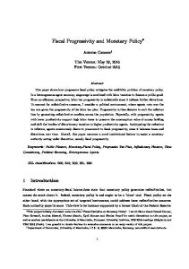
In‡ationary equilibrium. The green dotted lines in Figure 1 show the equilibrium in the ’in‡ationary regime’. As shown by the upper left subplot, the value function declines gently and almost linearly with the country’s debt burden, except for debt ratios very close to default when the slope increases sharply. The optimal default threshold equals b = 37:0% and is marked by a green circle. At that point, the government defaults. Following the exclusion period, it reenters capital markets with a debt ratio b = 20:7%. As regards nominal bond prices, Q (b), their gap with respect to the price of a riskless real bond (normalized to 1) re‡ects mainly expected in‡ation during the life of the bond as opposed to 38

We thus take the US CPI as the proxy for the ’World price’in the model. Notice also that, since the latter is normalized to 1, we target in‡ation di¤ erentials as opposed to in‡ation levels.

21

Bond price, Q

Value function, V

0.25

1

No in.ation

0.2

0.9

0.15 0.8 0.1 0.7 0.05 0.6 0 -0.05 -0.1

0.5

In.ationary 0

0.05

0.1

0.15

0.2

0.25

0.3

0.35

0.4

0.4

0

0.05

0.1

debt-to-GDP ratio, b

0.14

0.2

0.12

0

0.1

-0.2

0.08

-0.4

0.06

-0.6

0.04

-0.8

0.02

0

0.05

0.1

0.15

0.2

0.25

0.2

0.25

0.3

0.35

0.4

0.3

0.35

0.4

In.ation, :

Primary de-cit to gdp, c 0.4

-1

0.15

debt-to-GDP ratio, b

0.3

0.35

0

0.4

debt-to-GDP ratio, b

0

0.05

0.1

0.15

0.2

0.25

debt-to-GDP ratio, b

Figure 1: Equilibrium value function, bond price and policy functions.

22

Nominal yield, r

Real yield, r ! :

0.3

0.3

0.25

0.25

0.2

0.2

0.15

0.15

0.1

0.1

0.05

0

0.1

0.2

0.3

0.05

0.4

0

debt-to-GDP ratio, b

Default premium, r ! r~ 0.06

0.04

0.04

0.02

0.02

0

0.1

0.2

0.3

0.3

0.4

0

0.4

In.ationary

No in.ation 0

debt-to-GDP ratio, b

0.1

0.2

0.3

0.4

debt-to-GDP ratio, b

Expected time to default, T e

40

Drift, s

0.5 0

30

years

0.2

In.ation premium, r~ ! r7

0.06

0

0.1

debt-to-GDP ratio, b

-0.5 20 -1 10 0

-1.5

0

0.1

0.2

0.3

-2

0.4

debt-to-GDP ratio, b

0

0.1

0.2

0.3

0.4

debt-to-GDP ratio, b

Figure 2: Equilibrium yields, default and in‡ation premia, expected time-to-default and drift. default risk, except for debt ratios close to default. This can be seen more clearly in the second line of Figure 2, which displays how the gap between the nominal yield, r (b) = ( + ) =Q (b) , and the riskless real rate r is decomposed between the default and in‡ation premia, as de…ned in section 2.5. Indeed, for all b except those very close to b , bond yields re‡ect mostly the in‡ation premium, rather than the default premium, because default is still perceived as a very distant outcome, as re‡ected by an expected time-to-default of almost 40 years. It is only as debt approaches the default threshold that investors start perceiving default as rather imminent, demanding higher and higher default premia, which leads to the collapse of bond prices to their boundary value (Q(b ) = 0:44). The value function and bond prices, together with the state b, determine in turn the policy functions for in‡ation and primary de…cit, as described in equations (16) and (17). Regarding in‡ation, the government’s incentive to in‡ate debt away increases approximately linearly with the debt ratio. This is because the value function is approximately linear, such that the welfare gain 23

per unit of debt reduction is roughly constant. However, in the vicinity of the default threshold, the value function starts declining more and more steeply, such that a marginal reduction in the debt ratio yields a higher and higher marginal gain in welfare.39 As a result, optimal in‡ation increases steeply until reaching about 12% at the default threshold. Therefore, optimal monetary policy under discretion prescribes a roughly linear increase in in‡ation for moderate debt levels, and a strong increase as the economy approaches default. Finally, the primary de…cit ratio declines too in an almost linear fashion, re‡ecting the gentle decline in bond prices and the nearly constant slope of the value function. As debt approaches the default threshold, however, the sharp decline in bond prices leads the government to drastically reduce its primary de…cit, which actually turns to surplus once the economy gets su¢ ciently close to default. No-in‡ation equilibrium. Consider now the equilibrium in the ’no-in‡ation regime’, depicted by the solid blue lines in Figure 1. As explained in section 2.3.3, this scenario can be interpreted as the government issuing foreign currency debt or joining a monetary union with a very strong anti-in‡ationary commitment. Notice …rst that the optimal default threshold (b =0 = 37:2%; see blue circles) is essentially the same as in the baseline in‡ationary regime, for reasons that will become clear later. This means that the equilibrium range of debt ratios is basically the same in both regimes. The upper left plot of Figure 1 reveals our …rst main result: the value function is higher under no in‡ation for any debt ratio, even when the economy is close to default. The next subsection explains this result in detail. For now, notice that the no-in‡ation regime, apart from obviously avoiding the direct utility costs of in‡ation, implies also higher bond prices relative to the in‡ationary regime. This, from equation (16), leads the government to choose (slightly) higher primary de…cits, and hence higher consumption for given exogenous output. To understand why the no in‡ation regime delivers higher bond prices, or equivalently lower bond yields, we show in Figure 2 how the latter are decomposed between default and in‡ation premia. The no in‡ation regime raises default premia vis-à-vis the in‡ationary regime. This re‡ects the fact that default becomes more likely when the government gives up the ability to use in‡ation so as to stabilize its debt. However, the increase in default premia is very small compared with the reduction in in‡ation premia (to zero), which results in lower bond yields. The reason for such a small increase in default premia is that, for all debt ratios except those very close to b , default is still perceived as rather distant, as re‡ected by an expected time to default of about 30 years. As a result, the fact that investors expect default to happen somewhat sooner than in the in‡ationary regime (by about 8 years for most of the state space) is not enough to raise default 39

The increase in the slope (in absolute value) of the value function is hard to appreciate in Figure 1, because it only takes place at debt ratios very close to b . Zooming in the V (b) plot in the neighborhood of b reveals clearly such increase in the slope. The latter plot is available upon request.

24

premia signi…cantly. Notice also that ex post real yields r (b) (b) are actually higher in the in‡ationary regime for all debt ratios except those very close to default.40 The reason is that, in the in‡ationary regime, the negative e¤ect of the instantaneous in‡ation rate (b) on the real yield is more than compensated by the positive e¤ect of expectations of future in‡ation during the life of the (longterm) bond, which are priced into the nominal yield through the aforementioned in‡ation premium. It is only for b very close to b that instantaneous in‡ation is high enough to achieve lower real yields vis-à-vis the no in‡ation regime. Therefore, it is only when default is rather imminent that discretionary in‡ation helps push back the debt ratio. We will further elaborate on this and other ideas in the next subsection.

3.4

Understanding the costs and bene…ts of in‡ation

In order to gain further understanding of why social welfare is higher under zero in‡ation for any debt ratio, we decompose the value function (eq. 11) as V (b) = Vc (b) + Vcdef (b) + V (b) ; where Vc (b) = E0 Vcdef (b) = E0 V (b) = E0

(Z

(

T (b )

e

t

log(1 + c (bt ))dt + e

T (b )

+

0

maxf0; b +

T (b )

e

(Z

T (b )

e

t

0

2

^bg

+

(bt )2 dt + e

+

Vc ( b ) j b0 = b ; !

Vcdef ( b )

T (b )

+

)

)

j b0 = b ;

)

V ( b ) j b0 = b ;

and where dbt = s (bt ) dt

bt dWt ;

s (b) = r (b)

(b) +

2

b+

c (b) : Q (b)

The function Vc (b) represents the value of future consumption utility ‡ows (net of exogenous log output: remember that log(1 + c) = log C log Y ) enjoyed by households during repayment spells, Vc;def (b) measures the value of future (log)output losses during the exclusion spells that follow 40

As noted in the model section, the ex-post real yield, i.e. the di¤erent between r (b) and instantaneous in‡ation, is the real yield measure that is relevant for the dynamics of the debt ratio (see e.g. equation 22). A related concept would be the ex-ante real yield, i.e. the di¤erence between r (b) and expected in‡ation during the life of the bond. Both real yield measures would coincide if debt was instantaneous, but here they di¤er because bonds are long term.

25

defaults, and V (b) measures the value of future in‡ation disutility ‡ows. We can express these value functions recursively as 3 3 2 3 2 0 Vc (b) log(1 + c (b)) Vc (b) 2 7 ( b) 6 7 6 7 6 0 + = + s (b) (b) V (b) 0 V def 4 c 5 4 5 4 cdef 5 2 2 0 (b) V V (b) (b) 2 2

3 Vc00 (b) 7 6 00 4Vcdef (b)5 ; V 00 (b) 2

for b < b , with respective boundary conditions41 3 2 Vc (b ) 6 7 6 4Vcdef (b )5 = 4 V (b ) 2

0 maxf0;b +

0

3

^bg 7

5+

+

2

3 Vc ( b ) 6 7 4Vcdef ( b )5 : V ( b)

(24)

The costs and bene…ts of optimal discretionary in‡ation can be viewed through the lens of this decomposition. Let us begin with the costs. As discussed in the previous section, discretionary monetary policy su¤ers from an ’in‡ationary bias’: as long as there is a positive level of debt, the government cannot resist the temptation to in‡ate it away. As shown in Figure 1, the in‡ationary bias is sizable: the government chooses relatively high (…rst-order) in‡ation rates even at debt ratios relatively far away from the default threshold. This entails two kinds of costs. First, (instantaneous) in‡ation causes direct utility losses through the term 2 2 ; the expected discounted value of the stream of such losses is collected in the function V (b). Second, expectations of future in‡ation during the life of the bond depress nominal bond prices Q (b), which makes primary de…cit ratios c (b) more costly to …nance.42 This reduces primary de…cits relative to the zero in‡ation scenario, as seen in Figure 1, and hence it also reduces consumption (for given exogenous output). This second cost tends to reduce the value of the welfare component Vc (b) relative to its no-in‡ation counterpart. Let us now turn to the bene…ts. As is well known, when the government issues nominal noncontingent debt, unanticipated in‡ation makes ex-post real returns state-contingent.43 This is also true in our model: in‡ation surprises partially absorb the impact of output shocks on the debt ratio and thus improve consumption smoothing. The novelty here is that the possibility of a future sovereign default makes this shock-absorbing role even more valuable. Indeed, in response 41

The three value functions can be solved using numerical methods similar to those described in Appendix C. Notice that, since we have already solved for the optimal default threshold b , we do not need to impose smooth pasting conditions in order to solve for Vc (b), Vc;def (b) and V (b). 42 Also, lower nominal bond prices, or equivalently higher nominal bond yields r (b), tend do undo the bene…cial e¤ects of instantaneous in‡ation (b) on ex post real yields, r (b) (b). 43 The shock-absorbing role of state-contingent in‡ation has been extensively studied in the context of models that abstract from equilibrium sovereign default. See e.g. Chari, Christiano and Kehoe, 1991, Schmitt-Grohe and Uribe, 2004, and Siu, 2004, for analyses under commitment; and Niemann, Pichler and Sorger (2013) for a similar analysis under discretion.

26

Consumption utility, repayment spells

In.ation disutility

Consumption utility, default spells 0.15

0.15

0.2

0.1

0.1

0.15

0.05

0.05

0.1

0

0

0.05

-0.05

-0.05

0

-0.1

-0.1

No in.ation In.ationary

-0.05

0

0.05

0.1

0.15

0.2

0.25

0.3

debt-to-GDP ratio, b

0.35

0.4

0

0.05

0.1

0.15

0.2

0.25

0.3

0.35

0.4

debt-to-GDP ratio, b

0

0.05

0.1

0.15

0.2

0.25

0.3

0.35

0.4

debt-to-GDP ratio, b

Figure 3: Welfare decomposition to negative output shocks that bring the debt ratio closer to the default threshold, the government creates positive in‡ation surprises that partially undo the increase in the debt ratio. This way, monetary policy makes it less likely for the economy to fall in the default state, where social welfare is at its lowest due to the associated costs. The …rst of these costs is that the country temporarily loses its ability to smooth its consumption on account of its …nancial exclusion; the resulting ex ante welfare losses enter in the function Vc (b). The second cost is the drop in output (and hence in consumption) during the exclusion period; the ensuing ex ante welfare costs are collected in the function Vcdef (b). Figure 3 shows the contribution of each component to overall welfare in each monetary regime. The left plot shows Vc (b), i.e. the value of the stream of discounted utility ‡ows that households expect to enjoy during the current and all future repayment spells, given a current debt ratio b b . For relatively low debt ratios, the negative e¤ect of the in‡ationary bias on Vc (b) stemming from in‡ation premia dominates the positive e¤ect from state-contingent in‡ation. The opposite is true, however, when the economy is su¢ ciently close to default, for it is then that state-contingent in‡ation becomes most useful in postponing default and the resulting loss of the ability to smooth consumption. Moreover, Figure 1 shows that the primary de…cit ratio and hence consumption become more and more sensitive to the debt ratio as the latter approaches its default threshold. Thus, in response to a negative output shock that raises b, the ensuing positive in‡ation surprise contains the increase in b and hence the drop in consumption, the more so the closer b is to the default threshold.44 The middle plot in Figure 3 shows Vcdef (b), i.e. the value of the stream of discounted (log)output losses during all future default spells, given a current debt ratio b b . In this case, the contribution to welfare is higher for the in‡ationary regime for basically all debt ratios. This re‡ects the fact 44

In both regimes, the sharp increase in Vc (b) as b gets close to b re‡ects agents’anticipation of the fact that, once default …nally occurs and the country enters …nancial autarky, the large …scal surpluses (and the associated consumption cutbacks) su¤ered right before default are no longer necessary.

27

that, at a given debt ratio, default (and the associated output and consumption losses) is less likely to happen in the in‡ationary regime, thanks to the debt-stabilizing role of in‡ation explained before.45 Finally, the right plot in Figure 3 shows V (b), i.e. the value of all future discounted in‡ation disutility costs. The negative contribution in the in‡ationary regime increases slightly with the debt ratio, capturing the generally gentle increase in optimal in‡ation (see Figure 1).46 By comparing the three plots in Figure 3, we can now understand why discretionary in‡ation is detrimental at any debt ratio. For low debt ratios, there is little bene…t from state-contingent in‡ation, especially because default is still a distant outcome, and therefore the welfare costs from the in‡ationary bias dominate. As the debt ratio approaches the default threshold, the shockabsorbing bene…ts of state-contingent in‡ation become larger, but not large enough to dominate the in‡ation disutility costs. As a result, the welfare gap between both regimes narrows as the debt ratio increases, but never changes sign. At the respective default threshold, the no in‡ation regime continues to outperform the in‡ationary one. At that point, the value function equals V (b ) = Vdef (b ) =

maxf0; b +

^bg

+

+

V ( b );

which is precisely the sum of the three terminal values in (24). Since b is very similar in both cases, ^bg, as is the debt ratio at which the government so is the output loss from default, maxf0; b reenters capital markets following the exclusion period: b = 20:7%, versus b =0 = 20:8%.47 However, at such reentry ratio the value function is higher in the no-in‡ation regime, V =0 ( b =0 ) > V ( b ), precisely because it avoids the welfare costs of in‡ation.48 Therefore, welfare at default is higher under no in‡ation because it avoids the in‡ation costs to be incurred once the government reenters capital markets. To summarize this discussion, the no-in‡ation regime achieves superior welfare outcomes by avoiding the temptation to in‡ate at points of the state space where default is still perceived as rather distant, and hence where the stabilizing bene…ts from state-contingent in‡ation are relatively minor. Even at debt ratios close to default, the stabilizing bene…ts of in‡ation surprises remain comparatively small, re‡ecting the imminence of default. Therefore, abandoning the ability ^bg. Notice that, since b is almost identical in both regimes, so is the output loss from default: maxf0; b Therefore, the di¤erence in Vc;def (b) must be due to di¤erent default probabilities. 46 The increase in V (b) right before b re‡ects two opposing forces. On the one hand, optimal instantaneous in‡ation increases steeply at debt ratios very close to b , as shown in Figure 1; such an increase however is very short lived, because once b gets very close to b default happens rather quickly (see the expected time-to-default function in Figure 2). On the other hand, agents anticipate the fact that in‡ation will be zero during the imminent default spell. Numerically, the second e¤ect dominates. 47 ^b) in both Notice that b > ^b = 0:332 in both regimes. Thus, the loss in (log)output from default equals (b cases. 48 Notice that the sum of the two consumption-utility components, Vc (b) + Vc;def (b), is nearly identical in both regimes at the respective reentry ratio. 45

28

to in‡ate debt away eliminates the in‡ationary bias while barely worsening the sustainability of sovereign debt or, more generally, the ability to smooth consumption. The fact that debt sustainability is barely favored by in‡ation helps explain, in turn, why the optimal default threshold is so similar in both regimes.

3.5

Average performance

So far we have compared the two monetary policy regimes in terms of their welfare implications at each point of the state space, …nding that the no-in‡ation regime yields higher welfare at any debt ratio. It is also interesting to compare both regimes in terms of average welfare. The fact that one regime outperforms the other state by state does not guarantee that average welfare would be higher too. Since value functions are monotonically decreasing in both regimes, if the in‡ationary regime delivered su¢ ciently lower debt ratios most of the time, it could also achieve higher average welfare. In order to compute unconditional averages of welfare and other variables, we …rst need to solve for the stationary distribution of the debt ratio. For this purpose, it is useful to distinguish between (a) repayment spells and (b) the exclusion periods that follow each default. The stationary distribution conditional on being in a repayment spell, denoted by f (b), satis…es the following Kolmogorov Forward Equation (KFE), 0=

1 d2 d fs (b) f (b)g + ( b)2 f (b) + h (b 2 db 2 db

b)

h (b

b );

(25)

Rb with the constraint 1 = 0 f (b)db. In equation (25), the term h (b b ) re‡ects the fact that, following an exclusion spell, the government reenters the capital market at a debt ratio b = b , where ( ) is the Dirac ’delta’and h is a function of the average time spent in exclusion. Likewise, h (b b ) captures the fact that at b = b the government defaults and hence exits the conditional distribution f (b). Appendix F provides further details on how to obtain equation (25) and shows how to compute f (b) numerically, using an upwind …nite di¤erence scheme similar to the one employed to solve for the value and bond price functions. Figure 4 displays f (b) for both regimes. In the baseline regime, the possibility of using in‡ation to in‡ate debt away allows the government to shift the debt distribution slightly to the left vis-à-vis the no-in‡ation regime. Conditional on being in an exclusion period, we have already seen that primary de…cit and in‡ation are both zero, ct = t = 0. Since the rate at which the country reenters capital markets is constant at and hence independent of the time elapsed since default, we have that the value function and bond price are equal to their boundary values: Vt = V (b ) = Vdef (b ), Qt = Q (b ). Finally, we assume for simplicity that during the exclusion period the debt ratio is equal to b , i.e.

29

140

120

In.ationary 100

No in.ation 80

60

40

20

0 0.34

0.345

0.35

0.355

0.36

0.365

0.37

0.375

0.38

debt-to-GDP ratio, b

Figure 4: Stationary distribution of debt ratio, f (b): the ratio at which the country defaults.49 We can now compute the unconditional mean of each variable as the weighted average of the conditional means, using as weights the average time spent in repayment and exclusion periods. It is relatively straightforward to show that the stationary probability of being in repayment and e 1= exclusion periods equal P [bt < b ] = 1= T+T( eb( )b ) and P [bt = b ] = 1= +T e ( b ) , respectively. Thus, the unconditional mean of a variable xt equals E [xt ] = P [bt < b ] E [xt jbt < b ] + P [bt = b ] x Z b 1= T e( b ) x (b) f (b)db + x; = e 1= + T ( b ) 0 1= + T e ( b ) where x is the value of xt during the exclusion period.50 Table 2 displays average values of key model variables for both monetary regimes, as well as their corresponding empirical counterparts across EA periphery countries.51 Notice …rst that, remarkably, the no in‡ation regime (our model counterpart for the EMU period) replicates almost 49

We are thus assuming that during the exclusion/renegotiation period nominal debt outstanding is adjusted at each point in time to changes in the output endowment, such that the debt ratio is kept constant at b . We could alternatively assume that, during the exclusion period, nominal debt outstanding is kept constant at its value at the time of default (Bt^ ), such that the debt ratio changes with the output endowment. This would complicate the analysis while barely a¤ecting the numerical results, given the relatively short average duration of the exclusion period. 50 As explained above, c = 0, = 0, V = V (b ), and Q = Q (b ). 51 All data are annual except bond yields and default premia which are quarterly and annualized. We stop the sample for yields and default premia in 2012:Q2 (included) in order to isolate our analysis from the e¤ects of the annoucement by the European Central Bank of the Outright Monetary Transactions (OMT) programme in the summer of 2012.

30

exactly the average bond default premium (154 bp) conditional on being in a repayment spell (b < b ). In the in‡ationary regime, average bond yields (net of r = 400 bp) during repayment spells equal 446 bp, which re‡ects mostly average in‡ation premia (309 bp) rather than average default premia (137 bp). They are also signi…cantly higher than average yields under no in‡ation. Table 2. Averages values Data 1995-2012 units debt-to-GDP, b primary de…cit ratio, c in‡ation, bond yields (net of r), r r default premium, r r~ in‡ation premium, , r~ r Exp. time to default, T e Welfare loss, V V =0

% % % bp bp bp years % cons.

35.6 4.1 0.4 187 154 33 -

Model No in‡ation In‡ationary b < b uncond. b < b uncond. 35.6 0.5 0 153 153 0 29.5 0

35.8 0.5 0 315 315 0 0

35.6 0.4 3.2 446 137 309 37.1 -0.27

35.7 0.4 2.9 596 297 299 -0.26

Note: Data from IMF, national accounts, and Bloomberg. All data are annual except bond yields and default premia which are quarterly (annualized) and run through 2012:Q2. In‡ation is relative to the US. See Data Appendix for details. The German 10-year bond yield is used as empirical proxy for the riskless bond yield, r~. The column labelled ’b

< b ’displays results conditional on not being in exclusion, the column labelled ’uncond.’ displays fully

unconditional results. Welfare losses are relative to the no-in‡ation regime and are expressed in % of permanent consumption.

Interestingly, the fact that the no-in‡ation regime delivers lower average yields than the in‡ationary regime rationalizes the observed reduction in average sovereign yields across the EMU periphery brought about by the creation of the eurozone, if one interprets both regimes as the model counterparts of the EMU and pre-EMU periods respectively. Indeed, average yields on 10-year peripheral bonds decreased from 12.84% in the period 1987-94 to 5.87% in 1995-2012.52 Viewed through the lens of our model, this suggests that, when these countries decided to renounce the ability to in‡ate away their debts by joining EMU, the reduction in in‡ation expectations was a more important factor in investors’ pricing of the new euro-denominated bonds than the presumable increase in default risk. From a welfare perspective, we …nd that average welfare is lower in the in‡ationary regime, i.e. when the government in‡ates away its debt at discretion. The average welfare losses vis52

Notice that r = 5:87% = (r

r~) + (~ r

r) + r = 1:54% + 0:33% + 4%:

31

à-vis the no-in‡ation regime are equivalent to a reduction in permanent consumption of almost 0.3%. Therefore, the leftward shift in the debt distribution shown in Figure 4 is not su¢ cient to compensate for the fact that the value function is lower at any debt ratio. Such a small shift in the debt distribution re‡ects the low e¤ectiveness of discretionary debt in‡ation policies in our framework. Notice that optimal instantaneous in‡ation is relatively high in the range where the debt distribution accumulates more density, i.e. for b > 0:35.53 However, this is largely undone by the increase in nominal yields that goes along with higher in‡ation expectations. As a result, in the relevant debt range the in‡ationary regime achieves only marginally lower real yields, and hence only marginally slower debt accumulation, relative to the no in‡ation regime. Finally, we stress that the no in‡ation regime achieves higher average welfare despite the fact that it also implies higher debt ratios, which as explained before should work in the opposite direction given that value functions are monotonically decreasing. If anything, the comparison of average welfare underestimates the welfare gains from renouncing discretionary in‡ation, because it does not take into account the transition period that, starting from a common debt ratio, must elapse before the economy reaches its ergodic distribution in each policy regime. The state-bystate welfare comparison from the earlier sections precisely incorporates such transitional e¤ects and thus provides a more meaningful assessment, hence its prominence in our analysis.54

4

Robustness

We now evaluate the robustness of our main results to alternative calibrations of key model parameters. We will pay special attention to in‡ation and default costs, which arguably are key parameters for the purpose of the analysis here. As we will see, our main results on the welfare ranking between the no in‡ation and the in‡ationary regime continue to hold for a wide range of parameter values. The only exception is the case of very high output growth volatility ( ), which we analyze in section 4.3. Figure 7 in Appendix H displays the value functions in both regimes for alternative calibrations of structural parameters. As we show there, both value functions never cross for any of the cases considered. Therefore, our main result on the state-by-state welfare dominance of renouncing discretionary in‡ation policies is preserved for these alternative calibrations. In addition to this qualitative result, it is also interesting to quantify how the welfare gap between both regimes varies with structural parameters. And given the large number of calibrations considered, it is useful to synthesize such comparison by focusing on average welfare. Table 3 shows the average welfare 53

As shown in Figure 1, for b > 0:35 in‡ation is above 3%, with a maximum of around 12% in the limit as b ! b . For example, starting from a common debt ratio of b = 0:35, the welfare gap V =0 (b) V (b) is equivalent to 0.30% of permanent consumption, compared to the average welfare gap of 0.26% in Table 2. 54

32

losses from the in‡ationary regime in each calibration, together with averages of other relevant variables. We now discuss the robustness results for each structural parameter. Bond duration. The amortization rate determines the average Macaulay bond duration, 1= ( + r), for given riskless real return r. We consider bond durations of 3 and 7 years (compared to a baseline of 5 years). The welfare loss from using discretionary in‡ation decreases with bond duration. Intuitively, longer bond durations give more stability to the debt ratio, thus reducing the need to use debt in‡ation. This allows to reduce in‡ation premia in bond yields and direct utility costs, and hence the welfare loss relative to the no-in‡ation case. Bond recovery rate. The bond recovery parameter, , controls the average bond recovery rate after default, = ( ), for given reentry and trend growth rates ( ; ). We consider average recovery rates of 50% and 70% (the benchmark calibration is 60%). In this case, the welfare losses from discretionary in‡ation policies are fairly similar across di¤erent calibrations. As in the baseline calibration, the reduction in average in‡ation premia from giving up debt in‡ation clearly dominates the increase in average default premia. Household discount rate. In our baseline calibration, the household discount rate was set to 20% per annum. As discussed in the calibration section, the latter value is widely used in the quantitative sovereign default literature. However, one may wonder how robust our results are to making households, and hence the (benevolent) government, more patient. We consider discount rates of 10% and 6%.55 We …nd that, as households become more patient, the welfare loss from the in‡ationary regime increases. Intuitively, the more patient households are, the less they discount the utility costs that they may incur in the future when, following a default, their government reenters capital markets and starts in‡ating again. Duration of exclusion period. The reentry rate determines the average duration of the exclusion periods following default, 1= , set to 3 years in our benchmark calibration. We study the e¤ects of considering average durations of 2 and 5 years. In addition, we consider the relatively extreme case of a 40-year duration, which approximates the case of a permanent autarky following default. Table 3 reveals that our benchmark results remain mostly unchanged, even for quasi-permanent exclusion from capital markets. As we saw in the previous section, the welfare gap between both monetary regimes depends not so much on what happens in exclusion periods (during which output losses are fairly similar and in‡ation is zero in both cases), but on what happens while in repayment spells. As a result, changes in duration of the exclusion period do not signi…cantly alter the welfare gap between both regimes. 55

Our algorithm fails to converge in the in‡ationary case for discount rates and investor’s discount rate r below 1.7%.

33

below 5.7%, i.e. for gaps between

Table 3. Robustness analysis Welfare

Prim. de…cit

In‡ation

Nominal yield

Premia (bp)

Exp. time to

% cons.

ratio, %

%

net of r, bp

Default

In‡ation

default, years

No in‡ation

-

0.5

0

153

153

0

29.5

In‡ationary

-0.26

0.4

2.9

446

137

309

37.1

Benchmark

Average bond duration = 3 years No in‡ation

-

0.2

0

111

111

0

40.4

In‡ationary

-0.43

0.2

3.3

448

106

342

47.4

Average bond duration = 7 years No in‡ation

-

0.6

0

173

173

0

26.0

In‡ationary

-0.15

0.5

2.7

433

148

286

34.7

Bond recovery rate = 50% No in‡ation

-

0.6

0

174

174

0

30.8

In‡ationary

-0.25

0.5

3.0

466

154

312

38.6

Bond recovery rate = 70% No in‡ation

-

0.3

0

129

129

0

28.3

In‡ationary

-0.27

0.2

2.9

425

118

307

35.8

Default costs = 3:5% of GDP No in‡ation

-

0.6

0

152

152

0

29.8

In‡ationary

-0.09

0.5

1.8

329

142

187

34.5

Default costs = 7% of GDP No in‡ation

-

0.4

0

152

152

0

29.6

In‡ationary

-0.35

0.3

3.4

491

135

356

38.4

Household discount rate = 10% No in‡ation

-

-0.6

0

53

53

0

87.9

In‡ationary

-0.70

-0.6

3.2

374

46

328

115.2

Household discount rate = 6% No in‡ation

-

-0.7

0

22

22

0

209.5

In‡ationary

-1.26

-0.6

3.3

351

18

333

294.2

Note: Welfare is calculated with respect to the corresponding no-in‡ation scenario and is expressed in % of permanent consumption. Average values are unconditional for welfare, de…cit and in‡ation; for all other variables, averages are conditional on not being in exclusion (b

< b ). Benchmark calibration: average bond duration = 5

years, bond recovery rate = 60%, default cost = 6% of GDP, discount rate = 20%

34

Table 3 (cont’d). Robustness analysis Welfare

Prim. de…cit

In‡ation

Nominal yield

% cons.

ratio, %

%

net of r, bp

Scale in‡ation disutility

Premia (bp)

Exp. Time to

Default

In‡ation

default, years

= 6:40 (average in‡ation = 4%)

No in‡ation

-

0.5

0

153

153

0

29.5

In‡ationary

-0.34

0.4

4.0

551

133

419

40.0

Scale in‡ation disutility

= 13:99 (average in‡ation = 2%)

No in‡ation

-

0.5

0

153

153

0

29.5

In‡ationary

-0.18

0.4

2.0

352

142

210

34.6

= 8:33)

Slope of in‡ation eq.: Rotemberg = Calvo ( No in‡ation

-

0.5

0

153

153

0

29.5

In‡ationary

-0.26

-0.5

3.3

475

138

337

37.8

Average duration of exclusion period = 2 years No in‡ation

-

0.5

0

181

181

0

23.6

In‡ationary

-0.25

0.4

3.0

477

160

316

29.6

Average duration of exclusion period = 5 years No in‡ation

-

0.4

0

127

127

0

39.0

In‡ationary

-0.27

0.3

2.8

420

116

304

49.2

Average duration of exclusion period = 40 years No in‡ation

-

0.6

0

126

126

0

74.3

In‡ationary

-0.25

0.5

2.1

409

115

294

93.2

Volatility output growth = 10% No in‡ation

-

-0.7

0

285

285

0

15.7

In‡ationary

-0.08

-0.6

2.6

539

263

275

19.0

Volatility output growth = 20% No in‡ation

-

-1.2

0

279

279

0

16.2

In‡ationary

0.07

-1.1

2.4

519

262

257

19.1

Note: Welfare is calculated with respect to the corresponding no-in‡ation scenario and is expressed in % of permanent consumption. Average values are unconditional for welfare, de…cit and in‡ation; for all other variables, averages are conditional on not being in exclusion (b

< b ). Benchmark calibration: scale in‡ation disutility

= 9:15, average duration of exclusion period = 3 years, output growth volatility = 3.2%

35

4.1

In‡ation costs

In our baseline calibration, we set the scale parameter of in‡ation disutility, , in order for the in‡ationary model regime to replicate the in‡ation record in our target economies (see section 3.2). This delivered a baseline value of = 9:15, which produced an average in‡ation of 3.2% conditional on being in good credit standing, and 2.9% including exclusion spells. We now consider values of that deliver average in‡ation rates of 2% and 4%; this yields = 6:40 and = 13:99, respectively. We …nd that renouncing debt in‡ation continues to dominate in welfare terms. Interestingly, the welfare gap decreases with the scale of in‡ation disutility. This re‡ects two counteracting forces. On the one hand, a higher implies higher welfare costs for given in‡ation. On the other hand, costlier in‡ation reduces the in‡ationary bias of discretionary monetary policy and the associated welfare costs. Numerically, the second e¤ect is found to dominate. So far, we have used trend in‡ation rates so as to guide our choice of default cost. However, our microfoundations for in‡ation costs based on price adjustment costs à la Rotemberg (1982) o¤er us an alternative route. As it is well known, the Rotemberg (1982) and Calvo (1983) pricing models deliver isomorphic (linearized) in‡ation equations (the so-called ’New Keynesian Phillips curve’) that di¤er only in how their respective slope depend on the structural parameters. As shown in Appendix A, the slope of the in‡ation equation under Rotemberg pricing is " 1 , where " is the elasticity of individual …rm demand curves. It can also be shown that, in a continuous-time setup, the equivalent slope under Calvo pricing is ( + ), where is the price adjustment rate in that model (the proof is available upon request). It follows that, for the slope to be the same in both models, we need = (" +1 ) . Setting " to 11 (such that the gross markup "= (" 1) equals 1.10) and to 1 (such that prices last on average for 1 year), and given our calibration for the discount factor , we obtain = 8:33, such that in‡ation is somewhat less costly than in our baseline. Again, we …nd that our main results are preserved for this alternative calibration.

4.2

Default costs

As explained in our calibration section, the parameters and ^b in the default cost function, ^bg are chosen to produce a loss in output following default of 6%, which is roughly maxf0; b the midpoint of the range of values used in the literature. We now consider values of ^b such that, in equilibrium, output declines by 3.5% and 7% upon default.56 As shown in the table, the welfare losses from the in‡ationary regime increase with the output cost of defaults. Intuitively, the 56

We note that our model does not allow to compute the case of no default, e.g. by making it arbitrarily costly. The fact that households are more impatient than investors ( > r) implies that, absent default, the benevolent government would simply accumulate more and more debt over time, which would violate a standard no-Ponzi scheme condition.

36

Default costs

0.14

0.12

0.2

0.1

0.15

0.08

0.1

0.06

0.05

0.04

0

0

Exponential

0.02

-0.05

Benchmark 0

0.05

0.1

0.15

0.2

0.25

Value function, V

0.25

0.3

0.35

-0.1

0.4

debt-to-GDP ratio, b

0

0.05

0.1

0.15

0.2

0.25

0.3

0.35

0.4

debt-to-GDP ratio, b

Figure 5: Default costs and value function in the in‡ationary case for alternative default cost speci…cations. costlier it is to default, the higher the debt ratio at which the government optimally defaults and therefore the higher the debt ratios that are sustained in equilibrium. But higher debt ratios also imply higher in‡ation rates in the in‡ationary regime, with the resulting increase in welfare costs from the in‡ationary bias. Alternative functional form. We also check the robustness of our results to alternative functional form speci…cations for the (log)output losses from default. In particular, we consider the following functional form: e b 1 (b). Contrary to the baseline function, which has a kink at ^b and increases linearly thereafter, this speci…cation is a smooth, convex function of b. It also shares a number of plausible properties. First, (0) = 0, i.e. there is no cost of default if there is no debt to default upon. Second, (b) 0, i.e. default is costly: Third, 0 (b) 0, i.e. the cost should be increasing in the debt ratio that is defaulted upon. Finally, it only depends on two parameters ( ; ), and is thus equally parsimonious. As in our baseline calibration exercise, we choose and such that the no in‡ation regime replicates (i) the average ratio of external government debt over GDP across the EA periphery economies (35.6%) and (ii) an output decline of 6% following default. Since default costs a¤ect the equilibrium only through the value matching and smooth pasting conditions (equations 12 and 13), this is equivalent to imposing that the new cost function has the same value and slope at the

37

default threshold b =0 .57 Therefore, both cost speci…cations yield the exact same equilibrium in the no-in‡ation case by construction. However, since the default threshold is endogenous, both speci…cations may yield di¤erent equilibrium outcomes in the in‡ationary regime. The baseline and alternative default cost function are displayed in the left panel of Figure 5. As shown by the right panel, both speci…cations result in an almost identical value function also in the in‡ationary case.58 The reason is that, once again, the default threshold in the in‡ationary case (b = 36:98%) is very close to that in the no-in‡ation regime (b =0 = 37:20%), and hence so is the slope of the default costs at both thresholds, thus making the linear function (b ^b) a good approximation of e b 1 around b =0 . This conclusion also holds for other plausible default cost functions that satisfy the above properties, such as a 2-parameter polynomial approximation. This makes us con…dent about the robustness of our results to alternative functional forms.

4.3

Volatility of output shocks

As discussed in the calibration section, our baseline value for the volatility of shocks to output growth, = 3:2%, is calibrated to match the average growth volatility across peripheral EA economies since the creation of the euro. However, to the extent that one wants to extrapolate the present analysis to other geographical contexts, such as emerging market economies, one may want to consider higher levels of output growth volatility. The last panel of Table 3 shows the e¤ects of raising to 10%; for the purpose of illustration, we also consider an extremely large volatility of 20%. The average welfare gap between both regimes decreases with output volatility. Moreover, for output volatilities as high as 20%, the in‡ationary regime actually achieves higher average welfare relative to the no in‡ation regime, although the di¤erence is of second order. Figure 6 displays the value and policy functions for = 20%. As shown by the upper left panel, while the no in‡ation regime continues to dominate the in‡ationary one for most debt ratios, the opposite is true for debt ratios close to default. To understand this result, remember that state-contingent in‡ation allows the government to (partially) absorb the e¤ect of output shocks on the debt ratio, and hence on the probability of defaulting within a certain period of time. When the debt ratio is relatively far away from the default threshold, such a stabilizing role is relatively unimportant, even when output shocks are 57

That is,

and

must satisfy (b

=0

^b)

= =

(e e

b b

1);

=0 =0

;

where we have used the fact that, in the equilibrium with the baseline cost formulation, b =0 > ^b. For the values of and ^b in Table 1, we obtain = 25:02 and = 5:44 10 6 . 58 We only show the value function but the two models also produce identical policies and bond prices. Results are available upon request.

38

Value function, V

Primary de-cit to GDP, c

0 -0.05

0.4

No in.ation

0.2 0

-0.1

-0.2

In.ationary

-0.4

-0.15

-0.6 -0.2 -0.25 0.2

-0.8 0.25

0.3

0.35

-1 0.2

0.4

debt-to-GDP ratio, b 0.14

0.25

0.3

0.35

0.4

debt-to-GDP ratio, b

Expected time to default, T e

In.ation, :

25

0.12 20 0.1 15 years

0.08 0.06

10

0.04 5

0.02 0 0.2

0.25

0.3

0.35

0 0.2

0.4

debt-to-GDP ratio, b

0.25

0.3

0.35

0.4

debt-to-GDP ratio, b

Figure 6: Equilibrium with

= 20%:

very large. As a result, renouncing the use of in‡ation is relatively costless in terms of welfare, and the no in‡ation regime continues to outperform the in‡ationary one. But when the economy is relatively close to default and output growth is very volatile, the probability of defaulting within a relatively short period of time becomes much higher. This becomes apparent by comparing the expected time-to-default functions in Figure 6 with those under the baseline calibration (Figure 2). As a consequence, for debt ratios su¢ ciently close to default, the debt-stabilizing role of statecontingent in‡ation becomes important enough for the in‡ationary regime to actually deliver higher welfare.59 Moreover, because the economy defaults (and incurs the resulting costs) su¢ ciently less often under the in‡ationary regime, the latter is able to achieve higher welfare also on average. In any case, we emphasize that the degree of output growth volatility required in order for the in‡ationary regime to deliver higher welfare is high enough to be of little practical importance, even for emerging market economies.60 We thus conclude that, for realistic levels of output growth volatility, our main results regarding the desirability of renouncing the ability to conduct discretionary in‡ation policies remain robust. 59

Notice that this is despite the fact that the two arguments of the utility function, the primary de…cit ratio and in‡ation, continue to work in favor of the no in‡ation regime, as shown by Figure 6. 60 We have computed the threshold values of above which the in‡ationary regime delivers higher welfare (i) for at least some debt ratios and (i) on average, holding all other parameters at their baseline values. The thresholds are (i) 15.8% and (ii) 15.1%, respectively.

39

4.4

Monetary policy delegation

As explained in section 2.3.3, the no-in‡ation regime can be interpreted as the government issuing foreign currency debt, or joining a monetary union with a very strong anti-in‡ationary stance. We also argued that one could view the ’no in‡ation’regime as a situation in which the government appoints an independent central banker with an extremely great distaste for in‡ation. We may consider an intermediate arrangement by which the government delegates (discretionary) monetary policy to an independent central banker whose distaste for in‡ation is greater than that of society, but not so extreme as to choose zero in‡ation at all times. The question here is whether one can …nd intermediate preferences towards in‡ation that achieve better welfare outcomes than the two regimes considered thus far.61 Appendix J shows how the maximization problem is modi…ed when monetary policy is delegated to an independent authority. We compute average welfare for di¤erent degrees of central bank ’conservativeness’, as captured by the weight on in‡ation disutility in the central banker’s preferences (denoted by ~ ). We show that average social welfare increases monotonically with in‡ation conservativeness. The reason is that, as the degree of conservativeness increases, the welfare gains from reducing the in‡ationary bias outweigh the welfare losses from gradually renouncing in‡ation’s debt-stabilizing role. We also …nd however that average welfare is always lower than the one achieved by the no-in‡ation regime, which is reached only asymptotically (as ~ ! 1). Thus, while delegating monetary policy to a conservative central banker achieves better welfare outcomes relative to the case of a benevolent but discretionary policy-maker, such an institutional solution continues to be dominated by a scenario in which the government fully renounces the ability to in‡ate debt away, as would be exempli…ed e.g. by issuing foreign currency debt or joining a monetary union with a very strong and credible anti-in‡ationary mandate.

5

Conclusions

We have analyzed the welfare consequences of discretionary monetary policy, in a small open economy model where a benevolent government issues nominal debt without committing not to default on it and not to in‡ate it away. Our main focus has been to compare this scenario with an alternative regime in which the government e¤ectively renounces the option to in‡ate debt away, e.g. by issuing foreign currency debt or joining an anti-in‡ationary monetary union. We have found that giving up the option to in‡ate debt away achieves higher welfare at any 61

The analysis of monetary policy delegation as a means of alleviating in‡ationary bias problems has a longtradition in macroeconomics, going back at least to Rogo¤ (1985). See Niemann (2011) for a recent treatment of this question in a model where the in‡ationary bias stems from the existence of nominal noncontingent debt (as it does here) but that abstracts from sovereign default.

40

debt ratio. The reason lies in the costs and bene…ts of optimal discretionary in‡ation. On the one hand, state-contingent in‡ation partially absorbs the e¤ects of aggregate shocks on the debt ratio, which improves both consumption smoothing and sovereign debt sustainability. On the other hand, discretionary monetary policy features an in‡ationary bias, by which the government chooses positive in‡ation even when the economy is far away from default. This bias entails direct welfare costs, but also raises bond yields ceteris paribus, which makes (external) primary de…cits more costly to …nance and hence lowers consumption for given output. Abandoning the ability to in‡ate debt away eliminates the in‡ationary bias and the associated costs altogether, but also the bene…ts from in‡ation’s debt-stabilizing role. We have found that, for plausible calibrations, the …rst e¤ect dominates. Our results thus qualify the conventional wisdom according to which individual countries should bene…t from retaining the possibility of in‡ating away their sovereign debt, in the sense that such a bene…t may not materialize if governments in those countries cannot make commitments about future policy. Our …ndings may also rationalize why some emerging market economies with insu¢ cient in‡ation and repayment credibility issue their sovereign debt in a hard, foreign currency. Looking ahead, it would interesting to relax in future work some of our modelling assumptions, such as log consumption utility or default costs that depend only on the debt ratio. These were made in order to retain the very convenient feature of having a single state variable in the model (the debt ratio), which makes the analysis considerably more tractable. However, generalizing our framework to more ‡exible preferences and default cost speci…cation would allow for a more general assessment of the welfare implications of discretionary in‡ation in models of sovereign default. Likewise, we have analyzed the problem of a single government in a small open economy setup. Given our interest in recent developments in the euro area, we believe that extending the analysis presented here to the case of a monetary union with a common monetary authority and many national …scal authorities that di¤er in their outstanding sovereign debt levels is of great importance. We leave this task for future research.

References [1] Achdou, Y., J.-M. Lasry, P.-L. Lions and B. Moll (2015), "Heterogeneous Agent Models in Continuous Time," mimeo, Princeton University. [2] Aguiar, M., M. Amador, E. Farhi and G. Gopinath (2013). “Crisis And Commitment: In‡ation Credibility And The Vulnerability To Sovereign Debt Crises”, mimeo. [3] Aguiar, M., M. Amador, E. Farhi and G. Gopinath (2015). "Coordination And Crisis In Monetary Unions”, forthcoming, Quarterly Journal of Economics 41

[4] Aguiar, M. and G. Gopinath (2006), "Defaultable debt, interest rates and the current account," Journal of International Economics, 69(1), 64-83. [5] Araujo, A., M. Leon and R. Santos (2013), "Welfare analysis of currency regimes with defaultable debts," Journal of International Economics, 89(1), 143-153. [6] Arellano, C. (2008). "Default Risk and Income Fluctuations in Emerging Economies," American Economic Review, 98(3), 690-712. [7] Arellano, C. and J. Heathcote (2010). "Dollarization and …nancial integration", Journal of Economic Theory, 145(3), 944-973. [8] Arellano, C. and A. Ramanarayanan (2012). "Default and the Maturity Structure in Sovereign Bonds," Journal of Political Economy, 120(2), 187-232. [9] Bacchetta, P., E. Perazzi and E. van Wincoop (2015). Self-Ful…lling Debt Crises: Can Monetary Policy Really Help?, working paper [10] Barles, G. and P. E. Souganidis (1991), "Convergence of Approximation Schemes for Fully Nonlinear Second Order Equations," J. Asymptotic Analysis, 4, pp. 271-283. [11] Barro, R. J. and D. B. Gordon (1983). "A Positive Theory of Monetary Policy in a Natural Rate Model," Journal of Political Economy, 91(4), 589-610. [12] Ba¸sar, T. and G. J. Olsder (1999), (1999), Dynamic Noncooperative Game Theory, Ed. Society for Industrial and Applied Mathematics. 2 edition. [13] Benjamin, D. and M. L. J. Wright (2009), "Recovery Before Redemption: A Theory of Delays in Sovereign Debt Renegotiations", mimeo. [14] Bressan, A. (2010), Noncooperative di¤erential games, lecture notes. [15] Bressan, A. and K. T. Nguyen (2015), "A game theoretical model of debt and bankruptcy," mimeo. [16] Calvo, G. A. (1988), "Staggered prices in a utility-maximizing framework," Journal of Monetary Economics, 12(3), 383-398. [17] Calvo, G. A. (1988), "Servicing the Public Debt: The Role of Expectations," American Economic Review, 1988, 78, 647-661. [18] Calvo, G. A. and P. E. Guidotti (1993). "On the Flexibility of Monetary Policy: The Case of the Optimal In‡ation Tax," Review of Economic Studies, 60(3), 667-687. 42

[19] Camous, A. and R. Cooper (2014), "Monetary Policy and Debt Fragility", NBER Working Paper No. 20650. [20] Chari, V. V., L. J. Christiano and P. J. Kehoe, (1991), "Optimal Fiscal and Monetary Policy: Some Recent Results," Journal of Money, Credit and Banking, 23 (3), pp. 519-39. [21] Chatterjee, S. and B. Eyigungor (2012), "Maturity, Indebtedness, and Default Risk," American Economic Review, 102(6), 2674-99. [22] Cole, H. and T. Kehoe (2000), "Self-Ful…lling Debt Crises," Review of Economic Studies, 67, 91-116. [23] Corsetti, G. and L. Dedola (2014), "The Mystery of the Printing Press: Self-Ful…lling Debt Crises and Monetary Sovereignty," mimeo. [24] Crandall, M. G., H. Ishii, and P.-L. Lions (1992), “User’s guide to viscosity solutions of second order partial di¤erential equations.”ArXiv Mathematics e-prints. [25] Crandall, M. G., and P.-L. Lions (1983), “Viscosity Solutions of Hamilton-Jacobi Equations.” Transactions of the American Mathematical Society, 277(1), pp. 1–42. [26] Cruces, J.J., Buscaglia, M., Alonso, J. (2002), "The term structure of country risk and valuation in emerging markets," Manuscript, Universidad Nacional de La Plata. [27] Cruces, J., and Trebesch, C., (2011), "Sovereign Defaults:The Price of Haircuts," CESifo Working Paper 3604. [28] Da-Rocha, J. M., E. L. Giménez and F. X. Lores, 2013. "Self-ful…lling crises with default and devaluation," Economic Theory, 53(3), 499-535. [29] Dias, D. A. and C. Richmond (2007), "Duration of Capital Market Exclusion: An Empirical Investigation," Working Paper, UCLA. [30] Diaz-Gimenez, J., G. Giovannetti, R. Marimon and P. Teles (2008). "Nominal Debt as a Burden on Monetary Policy," Review of Economic Dynamics, 11(3), 493-514. [31] Dixit, A. and R. S. Pindyck (1994), Investment under Uncertainty, Princeton University Press. [32] Dockner, E. J., S. Jorgensen, N. V. Long and G. Sorger (2000), Di¤erential Games in Economics and Management Science, Ed. Cambridge University Press. [33] Doraszelski, U. and K. L. Judd (2012). "Avoiding the curse of dimensionality in dynamic stochastic games," Quantitative Economics, 3 (1), pp. 53-93. 43

[34] Du, W. and J. Schreger (2015). "Sovereign Risk, Currency Risk, and Corporate Balance Sheets", mimeo [35] Eaton, J. and M. Gersovitz (1981), "Debt with Potential Repudiation: Theoretical and Empirical Analysis," Review of Economic Studies, 48(2), 289-309. [36] Faraglia, E., A. Marcet, R. Oikonomou and A. Scott (2013), "The Impact of Debt Levels and Debt Maturity on In‡ation," Economic Journal, 123 (566), pp. F164-F192. [37] Hatchondo, J. C. and L. Martinez (2009), "Long-duration bonds and sovereign defaults," Journal of International Economics, 79(1), 117-125. [38] Kydland, F. E. and E. C. Prescott. 1977. "Rules Rather Than Discretion: The Inconsistency of Optimal Plans," Journal of Political Economy, 85, 473-91. [39] Martin, F. (2009). "A positive theory of government debt", Review of Economic Dynamics, 12(4), 608–631 [40] Mendoza, E. and V. Z. Yue (2012). "A General Equilibrium Model of Sovereign Default and Business Cycles," Quarterly Journal of Economics, 127(2), 889-946. [41] Niemann, S. (2011). "Dynamic monetary–…scal interactions and the role of monetary conservatism," Journal of Monetary Economics, 58(3), 234-247. [42] Niemann, S., P. Pichler and G. Sorger (2013). "Public debt, discretionary policy, and in‡ation persistence," Journal of Economic Dynamics and Control, 37(6), 1097-1109. [43] Nuño, G. and B. Moll (2015), "Controlling a Distribution of Heterogeneous Agents," mimeo. [44] Øksendal, B. and A. Sulem (2007). Applied Stochastic Control of Jump Di¤usions. Springer. [45] Reis, R. (2013). "The Mystique Surrounding the Central Bank’s Balance Sheet, Applied to the European Crisis," American Economic Review, 103(3), 135-40. [46] Rogo¤, K. (1985), “The Optimal Degree of Commitment to an Intermediate Monetary Target,”Quarterly Journal of Economics, 100(4), 1169–89. [47] Rotemberg, J. J. (1982). "Sticky Prices in the United States," Journal of Political Economy, 90(6), 1187-1211. [48] Röttger, J. (2016). "Monetary and Fiscal Policy with Sovereign Default", mimeo. [49] Schmitt-Grohe, S. and M. Uribe (2004). "Optimal …scal and monetary policy under sticky prices," Journal of Economic Theory, 114 (2), pp. 198-230. 44

[50] Stokey, N. (2009). The Economics of Inaction, Princeton University Press. [51] Siu, H. (2004). "Optimal …scal and monetary policy with sticky prices," Journal of Monetary Economics, 51(3), 575-607. [52] Soner, H. M. (1986a), “Optimal Control with State-Space Constraint I,” SIAM Journal on Control and Optimization, 24(3), pp. 552–561. [53] Soner, H. M. (1986b), “Optimal Control with State-Space Constraint II,” SIAM Journal on Control and Optimization, 24(6), pp. 1110–1122. [54] Sunder-Plassmann, L. (2014). "In‡ation, default, and the denomination of sovereign debt", mimeo. [55] Woodford, M. (2001). "Fiscal Requirements for Price Stability," Journal of Money, Credit and Banking, 33(3), 669-728. [56] Yue, V. Z. (2010). "Sovereign default and debt renegotiation," Journal of International Economics, 80(2), 176-187.

45

Online appendix (not for publication) A. An economy with costly price adjustment In this appendix, we lay out a model economy with the following characteristics: (i) …rms are explicitly modelled, (ii) a subset of them are price-setters but incur a convex cost for changing their nominal price, and (iii) the social welfare function and the equilibrium conditions are the same as in the model economy in the main text. Final good producer In the model laid out in the main text, we assumed that output of the single consumption good Yt is exogenous. Consider now an alternative setup in which the single consumption good is produced by a representative, perfectly competitive …nal good producer with the following Dixit-Stiglitz technology, Z 1 "=(" 1) (" 1)=" ; (26) yit di Yt = 0

where fyit g is a continuum of intermediate goods and " > 1. Let Pit denote the nominal price of R1 intermediate good i 2 [0; 1]. The …rm chooses fyit g to maximize pro…ts, Pt Yt Pit yit di, subject 0 to (26). The …rst order conditions are yit =

Pit Pt

"

Yt ;

(27)

for each i 2 [0; 1]. Assuming free entry, the zero pro…t condition and equations (27) imply Pt = R1 ( 0 Pit1 " di)1=(1 ") . Intermediate goods producers Each intermediate good i is produced by a monopolistically competitive intermediate-good producer, which we will refer to as ’…rm i’henceforth for brevity. Firm i operates a linear production technology, yit = Zt nit ; (28) where nit is labor input and Zt is productivity. The latter is assumed to follow a geometric Brownian motion, dZt = Zt dt + Zt dWt : (29) At each point in time, …rms can change the price of their product but face quadratic price adjustment cost as in Rotemberg (1982). Letting P_ it dPit =dt denote the change in the …rm’s price, 46

price adjustment costs in units of the …nal good are given by

t

!

P_it Pit

P_it Pit

2

!2

C~t ;

(30)

where C~t is aggregate consumption. Let it P_it =Pit denote the rate of increase in the …rm’s price. The instantaneous pro…t function in units of the …nal good is given by Pit yit Pt Pit = Pt

wt nit

=

it

wt Zt

(

t

it ) "

Pit Pt

Yt

t

(

(31)

it ) ;

where wt is the perfectly competitive real wage and in the second equality we have used (27) and (28). Without loss of generality, …rms are assumed to be risk neutral and have the same discount factor as households, . Then …rm i’s objective function is E0

Z

1

e

t

it di;

0

with it given by (31). Notice that the …rm’s optimization problem is not a¤ected by sovereign defaults, although of course default does a¤ect the aggregate variables that enter the …rm’s problem (Yt ; Pt , etc.). The state variable speci…c to …rm i, Pit , evolves according to dPit = it Pit dt. We conjecture that the aggregate state relevant to the …rm’s decisions can be summarized by (bt ; Zt ; Pt ) St .62 Then …rm i’s value function J (Pit ; St ) must satisfy the following HamiltonJacobi-Bellman (HJB) equation, J (Pi ; S) = max i

+

0 S

(

Pi P

w Z

"

Pi P

(S) DS J (Pi ; S) +

Y 1 2

0 S

@J ( i ) + i Pi (Pi ; S) @Pi

(S) (DSS J (Pi ; S))

S

)

(S) ;

where the vectors ( S (S) ; S (S)) collect the drift and di¤usion terms, respectively, of the aggregate states S, and (DS ; DSS ) are the gradient and Hessian operators, respectively, with respect to S.63 The …rst order and envelope conditions of this problem are (we omit the arguments of J to In particular, we later show that in equilibrium Yt = Zt , whereas wt and C~t are also functions of (bt ; Zt ; Pt ). The states Pt and bt follow the same laws of motion as in the main text, equations (2) and (4) respectively, whereas Zt follows equation (29). 63 In particular, S (S) = [s (b) ; Z; P ]0 , where s (b) is the drift of the debt ratio b as de…ned in section 2.5 of the main text; and S (S) = [ b; Z; 0]0 . 62

47

ease the notation), ~ = Pi @J ; @Pi

iC

@J = @Pi

"

w Pi Pi (" 1) Z P P @ 1 0 + S (S) DS J + @Pi 2 "

0 S

Y + Pi

@J @ 2J + Pi 2 @Pi @Pi

i

(S) (DSS J)

S

(S) :

In what follows, we will consider a symmetric equilibrium in which all …rms choose the same price: Pi = P; i = for all i. After some algebra, it can be shown that the above conditions imply the following pricing Euler equation,64 C~b (b; Z) s (b) + C~Z (b; Z) Z C~ (b; Z)

!

(b) =

"

1

" "

w 1Z

1

Z + s (b) ~ C (b; Z)

0

(b)

+ 2 F (S) :

(32)

where C~ (b; Z) and (b) denote the equilibrium policy functions for total spending and in‡ation, and F (S) is a function of the aggregate state; in particular, the term 2 F (S) captures the e¤ect of aggregate uncertainty on …rms’pricing decision.65 Equation (32) determines the market clearing wage w as a function of S. Households The representative household’s preferences are given by E0

Z

1

e

t

log C~t dt;

0

64 65

The proof is available upon request. In the special case with no aggregate uncertainty, = 0, equation (32) simpli…es to 0 : 1 ~ CA " 1 " w Z @ = 1 + _; " 1Z C~ C~

~ where we have used the fact, in this case, s (b) = db=dt and Z = dZ=dt, which implies C~b s (b)+ C~Z Z = dC=dt and 0 (b) s (b) = d =dt _ .

48

:

C~

where C~t is household consumption of the …nal good. De…ne total real spending as the sum of household consumption and price adjustment costs, Ct

C~t +

Z

1 t

(

it ) di

0

= C~t +

2~ t Ct ;

2

(33)

where in the second equality we have used the de…nition of t (eq. 30) and the symmetry across …rms in equilibrium. Instantaneous utility can then be expressed as log(C~t ) = log (Ct )

log 1 +

2

2 t 2

= log (Ct )

2 t

2

+O

2

2 t

!

;

(34)

where O(kxk2 ) denotes terms of order second and higher in x. Expression (34) is the same as the utility function in the main text (eq. 6), up to a …rst order approximation of log(1 + x) around x = 0, where x 2 2 represents the percentage of aggregate spending that is lost to price adjustment. For our baseline calibration ( = 9:15), the latter object is relatively small even for relatively high in‡ation rates, and therefore so is the error in computing the utility losses from price adjustment.66 Therefore, the utility function used in the main text provides a fairly accurate approximation of the welfare losses caused by in‡ation in the economy with costly price adjustment described here. In Appendix I, we solve the equilibrium implied by the exact in‡ation disutility function in the …rst line of equation (34) and show that the results are virtually identical to those in the main text. As in the model in the main text, the government rebates to the household all the net proceedings from its international credit operations, denoted by Tt in nominal terms. We assume that the household supplies one unit of labor input inelastically: nt = 1. It also receives …rms’pro…ts in a lump-sum manner. Thus the household’s nominal budget constraint is Pt C~t = Pt wt + Pt

Z

1 it di

+ Tt :

0

In the symmetric equilibrium, each …rm’s labor demand is nit = yit =Zt = Yt =Zt . Since labor supply 66

For instance, for an in‡ation rate as high as = 12% (the maximum equilibrium in‡ation rate obtained in the in‡ationary regime), the exact and the approximated price adjustment cost are log(1 + 2 2 ) = 6:38% and 2 = 6:59% of aggregate spending, respectively. 2

49

equals one, labor market clearing requires Z

1

0

nit di = Yt =Zt = 1 , Yt = Zt :

Therefore, in equilibrium output is simply equal to exogenous productivity Zt . Each …rm’s real pro…ts equal it = Yt wt 2 2t C~t . Using this in the household’s budget constraint, we obtain Tt = Pt C~t +

2

2~ t Ct

Yt

= Pt (Ct

Yt ) ;

where in the second equality we have used (33). Therefore, the primary de…cit ratio is ct

C t Yt Tt = ; P t Yt Yt

as in the main text. It follows that log (Ct ) = log (1 + ct ) + log (Yt ), such that household welfare can be expressed as a function of the policy variables (ct ; t ) as in equation (7) in the main text. Fiscal and monetary policy The government maximizes household welfare subject to the laws of motion of the aggregate state variables. The default scenario is the same as in the main text, with one quali…cation: upon default at a debt ratio bt , and during the subsequent exclusion period, productivity equals Zt exp[ maxf0; bt ^bg]. This, together with the fact that in equilibrium Yt = Zt , implies that the default scenario is exactly as in the main text. It is then trivial to show that the government’s maximization problem is exactly the same as in the main text, once we take into account that (i) the welfare criterion is the same (equation 11), and (ii) the law of motion of the debt ratio is the same (equation 4). As a result, the policy functions for in‡ation and primary de…cit ratio will also be the same: t = (bt ), ct = c (bt ). Notice …nally that, since Yt = Zt , in equilibrium we have Ct = (1 + c (bt )) Zt C (bt ; Zt ), 2 ~ ~ C (bt ; Zt ). Likewise, the pricing Euler equation and therefore Ct = C (bt ; Zt ) =[1 + 2 (bt ) ] derived above (equation 32) determines the market clearing wage given the aggregate state: wt = w (Zt ; bt ; Pt ). We thus verify our previous conjecture that (bt ; Zt ; Pt ) are the relevant aggregate states for …rms.

B. Proof of Proposition 2 Consider the no-in‡ation regime with = 0: We …rst conjecture that there is a stable steady state, that is, a point bss 2 [0; b ) such that s (bss ) = 0 and s0 (bss ) < 0. Then, there is an interval around 50

bss with radius " > 0 such that, for any initial value b0 2 (bss "; bss + "), bt converges to bss and remains there forever.67 In that interval default cannot happen and therefore the price of the bond + , which implies Q0 (b) = 0 for all b 2 (bss "; bss + "). The envelope is constant at Q (b) = +r condition of the HJB equation is V 0 (b) =

+ Q(b)

[( + ) b + c]

Q0 (b) Q2 (b)

V 0 (b) + s (b) V 00 (b):

(35)

In the stable steady state, the above condition simpli…es to (

r + ) V 0 (bss ) = 0;

+ and Q0 (bss ) = 0: From the Proof where we have used the fact that s (bss ) = 0, Q (bss ) = +r of Proposition 1 in the main text, V 0 (b) cannot be zero in equilibrium for any b 2 [0; b ). Also, Condition 1 implies ( r + ) > 0. Therefore, the envelope condition (35) is not satis…ed at the conjectured stable steady-state ratio bss . Therefore the initial conjecture is false: there is no stable steady-state.68 Assume instead that there is an unstable steady state bss 2 (0; b ) with s (bss ) = 0 and s0 (bss ) > 0: Since we have already proved that there is no stable steady state, it must be the case that, for any initial b0 < bss , s (b0 ) < 0 and therefore bt converges to zero. However, at b = 0 the state constraint b 0 implies s (0) 0: If s (0) is non negative, b = 0 is not a stable steady state (s0 (0) 0) and s (b) does not cross zero until b = bss then s (b0 ) cannot be negative for any b0 2 (0; bss ).69 Hence there can be no unstable steady-state.70 Notice that bss = 0 is not considered, as we cannot rule out the case s (0) = 0 and s0 (0) > 0: Assume that there is a steady-state s (bss ) = 0 with s0 (bss ) = 0 and s00 (bss ) 6= 0: In this case, depending on the concavity of s (b) there will be either a left- or a right-interval including bss such that, for any initial value b0 in that interval, bt converges to bss and default cannot happen. If we take the limit as b ! bss of (35) in this half-interval the envelope condition is again not satis…ed and thus we can also rule out this possibility.71 Finally, if s (bss ) = s0 (bss ) = s00 (bss ) = 0 there are two possible cases. Provided that s000 (bss ) < 0 67

In the case of bss = 0; this is an interval [0; "): This result also holds if the drift s(b) is discontinuous around bss but s(bss ") > 0 and s(bss + ") < 0 as the + price of the bond is constant in the interval: Q (bss ) = +r and Q0 (bss ) = 0 and the envelope condition (35) is not satis…ed. 69 This implicitly assumes that s (b) is continuous in the subinterval. If this were not the case, that is, if there was a discontinuity at some b1 2 (0; bss ) such that s(b) jumps from the positive to the negative region at b1 , then b1 would be a stable steady state, a possibility that had already been discarded. 70 Again, the proof is similar in the case of a discontinuity at bss with the drift jumping from the.negative to the positive region. 71 The result also holds if the drift s(b) is discontinuous around bss but s(bss ") < 0 and s(bss + ") > 0 following the same line of reasoning as above. 68

51

then the steady state is stable and we are back in the …rst part of the proof. If s000 (bss ) > 0 then the steady-state is unstable and we are in the second part of the proof. In any case no steady-state is possible. We can procced with higher order derivatives, but the proof will always fall in any of the two previous cases. The conclusion is that, given Condition 1 and the envelope condition (35), there is no steadystate with positive debt, s (b) 6= 0 8b 2 (0; b ). And since s(0) 0, we have s(b) > 0 8b 2 (0; b ). QED.

C. Numerical algorithm We describe the numerical algorithm used to jointly solve for the equilibrium value function, V (b), and bond price function, Q (b). The algorithm proceeds in 3 steps. We describe each step in turn. Step 1: Solution to the Hamilton-Jacobi-Bellman equation The HJB equation (14) is solved using an upwind …nite di¤erence scheme following Achdou et al. (2015). It approximates the value function V (b) on a …nite grid with step b : b 2 fb1 ; :::; bI g, where bi = bi 1 + b = b1 + (i 1) b for 2 i I. The bounds are b1 = 0 and bI = b b, such that b = b =I. We choose such that (I + 1) 2 N. We use the notation Vi V (bi ); i = 1; :::; I, and similarly for the bond price function Qi and the policy functions ( i ; ci ). Notice …rst that the HJB equation involves …rst and second derivatives of the value function, 0 V (b) and V 00 (b). At each point of the grid, the …rst derivative can be approximated with a forward (F ) or a backward (B) approximation, V 0 (bi )

@F Vi

V 0 (bi )

@B Vi

Vi+1 Vi

Vi b Vi b

1

;

(36)

;

(37)

whereas the second derivative is approximated by V 00 (bi )

@bb Vi

Vi+1 + Vi 1 ( b)2

2Vi

(38)

:

In an upwind scheme, the choice of forward or backward derivative depends on the sign of the drift function for the state variable, given by s (b)

+ + Q (b)

2

(b) b +

52

c (b) ; Q (b)

(39)

for b

b , where Q(b) 1; V 0 (b) b 0 bQ(b) V (b) = : (1 + c)

c (b) = ( ) =

Let superscript n denote the iteration counter. The HJB equation is approximated by the following upwind scheme, Vin+1

Vin

+ Vin+1 = log(cni +1)

2

( n+1 n n 2 si;F 1sni;F >0 +@B Vin+1 sni;B 1sni;B <0 + i ) +@F Vi

(

bi )2 @bb Vin+1 ; 2

for i = 1; :::; I, where 1 ( ) is the indicator function and + + Qi + + Qi

sni;F = sni;B =

2

+

2

+

bi

@F Vin bi

bi

@B Vin bi

1 1 + n @F V i Qi 1 1 + n @B Vi Qi

; :

Therefore, when the drift is positive (sni;F > 0) we employ a forward approximation of the derivative, @F Vin+1 ; when it is negative (sni;B < 0) we employ a backward approximation, @B Vin+1 . The term Vin+1 Vin

! 0 as Vin+1 ! Vin : Moving all terms involving V n+1 to the left hand side and the rest to the right hand side, we obtain Vin+1 1

n i

+ Vin+1

n i

n+1 + Vi+1

n i

= log(cni + 1)

2

(

n 2 i)

+

Vin

;

(40)

where n i

n i

n i

sni;B 1sni;B <0 b 1

+ +

( bi )2 ; 2 ( b)2 sni;F 1sni;F >0 sni;B 1sni;B <0 b

sni;F 1sni;F >0 b

b

( bi )2 + ; ( b)2

2

( bi ) ; 2 ( b)2

for i = 1; :::; I. Notice that the state constraint b 0 means that sn1;B = 0, which together with b1 = 0 implies n1 = 0. In equation (40), the optimal primary de…cit ratio is set to cni

=

Qni @Vin

53

1 ;

(41)

where

Q(bi ) 1sn 1 + ci i;F

@Vi = @F Vi 1sni;F >0 + @B Vi 1sni;B <0

In the above expression, ci is the consumption level such that s (bi ) + + Qi

bi Q i (1 + ci )

2

bi +

: 0 1s n i;B 0 sni = 0, i.e. it solves

ci = 0: Qi

The solution is the higher root of the above equation, (1 +

i Qi ) +

ci = where

i

+ Q(bi )

+

r

(1 +

2 i Qi )

4

2

h

i Qi

b2i Q2i

i

;

bi . Given cni , the optimal in‡ation rate is

2

n i

bQi : (1 + cni )

=

(42)

The smooth pasting boundary condition (equation 13) can be approximated by72 n+1 VI+1

VIn+1 = b

+

+

+

n+1 @F V n(I+1) ) VI+1 = VIn+1 +

+

+

@F V n(I+1)

+

b: (43)

Equation (40) is a system of I linear equations which can be written in matrix notation as: An Vn+1 = dn ;

(44)

where the matrix An and the vectors Vn+1 and dn are de…ned by 2

6 6 6 6 6 An = 6 6 6 6 4

n 1 n 2

n 1 n 2 n 3

0 .. .

..

0 0

0 0

.

0 n 2 n 3

..

.

0 0 n 3

..

.

n I 1

0

..

.

n I 1 n I

3

0 0 0 .. . n I 1 n I

+

n I

2

V1n+1 V2n+1 V3n+1 .. .

7 6 7 6 7 6 7 6 7 6 7 ; Vn+1 = 6 7 6 7 6 7 6 n+1 5 4 VI 1 VIn+1

3 7 7 7 7 7 7 7 7 7 5

(45)

72 Notice that we solve for the value function under the guess that the optimal default threshold satis…es b > ^b, ^bg = b ^b. We verify that our guess is satis…ed in equilibrium in all our simulations. such that maxf0; b

54

2

6 6 6 6 6 n d =6 6 6 6 6 4

log(cn1 + 1) log(cn2 + 1) log(cn3 + 1)

2 2

.. .

log(cnI 1 + 1) log(cnI + 1)

n 2 2

I

+

2

n 2 1) n 2 2) n 2 3)

( ( (

VIn

+

I

n I

1

3

V1n V2n V3n

2

n 2

+ + +

+

+

Vn I

+

1

@F V n(I+1)

b

7 7 7 7 7 7: 7 7 7 7 5

Notice that the element (I; I) in A is nI + nI due to the smooth pasting condition (43).73 The algorithm to solve the HJB equation runs as follows. Begin with an initial guess Vi0 = i = 1; :::; I. Set n = 0: Then:

bi ,

1. Compute @F Vin ; @B Vin and @bb Vin using (36)-(38). 2. Compute cni and

n i

using (41) and (42).

3. Find Vin+1 solving the linear system of equations (44). 4. If Vin+1 is close enough to Vin ; stop. If not set n := n + 1 and go to 1. Step 2: Solution to the Bond Pricing Equation The pricing equation (19) is also solved using an upwind …nite di¤erence scheme. The equation in this case is Q(b) (r + (b) + ) = ( + ) +

+ + Q(b)

2

(b) b +

c(b) ( b)2 00 Q (b); Q0 (b) + Q(b) 2

with a boundary condition Q(b ) =

r

Q( b ):

+

This case is similar to the HJB equation. Using the notation Qi = Q(bi ); the equation can be expressed as Qn+1 i

Qni

+

Qn+1 i

73

(r +

Note that in the case Bellman equation

i

1

+ )=

+ +

@F Qn+1 sni;F 1sni;F >0 i

+

@B Qn+1 sni;B 1sni;B <0 i

( bi )2 + @bb Qn+1 ; i 2 (46)

! 0 this is just a standard policy iteration algorithm on the discrete state-space V = u+ (1

where =

1 (1

)

and A = limn!1 An :

55

) (I

V; A) ;

where: Q0 (bi )

@F Qi

Q0 (bi )

@B Qi

Q00 (bi )

@bb Qi

Qi+1

Qi

; b Qi Qi 1 ; b Qi+1 + Qi 1 ( b)2

2Qi

and rearranging terms Qn+1 i 1

n i

+ Qn+1 ( i

n i

+r+

i

) + Qn+1 i+1

+

n i

=

+ +

QI+1 =

Qni

; 8i < I + 1; Q( (I + 1)):

+

Notice the abuse of notation, as +

sni;F = sni;B = sni =

Qn (b

i)

+

2

i

bi +

ci n Q (b

i)

:

Equation (46) is again a system of I linear equations which can be written in matrix notation as: Fn Qn+1 = qn ;

(47)

where the matrix Fn and the vectors Qn+1 and f n are de…ned by: 2

( n1 + 6 6 + +r 6 6 6 n 6 2 6 6 6 6 0 6 n F =6 6 6 .. 6 . 6 6 6 0 6 6 6 6 4 0

1

)

n 1

( n2 + + +r n 3

...

2

)

0

0

n 2

0

( n3 + + +r ...

3

0

) ...

0

( nI 1 + + +r

0

n I

56

3

... I 1

)

n I 1

( nI + + +r

I

)

7 7 7 7 7 7 7 7 7 7 7 7; 7 7 7 7 7 7 7 7 7 7 5

2

Qn+1

Qn+1 1 Qn+1 2;1 Qn+1 3;1 .. .

6 6 6 6 6 =6 6 6 6 n+1 4 QI 1 Qn+1 I

3

2

7 7 7 7 7 7; 7 7 7 5

+ + + + + + .. .

6 6 6 6 6 n q =6 6 6 6 4

+ + + +

Qn I

Qn 2 Qn 3

Qn

n I

3

Qn 1

I

1

Qn(I+1)

+

7 7 7 7 7 7: 7 7 7 5

The algorithm to solve the bond pricing equation is similar to the HJB. Begin with an initial guess Q0i = r++ , set n = 0: Then: 1. Find Qin+1 solving the linear system of equations (47). 2. If Qn+1 is close enough to Qni ; stop. If not set n := n + 1 and go to 1. i Step 3: Value Matching Finally, we iterate until the value matching condition (12) is satis…ed: n max 0; bI+1

VI+1 =

o ^b

+

+

+

V

(48)

(I+1) :

Taking into account (43), condition (48) can be rewritten as

VI +

+

+

+

@F V

b+

(I+1)

n max 0; bI+1

o ^b

+

+

V

(I+1)

= 0:

D. The riskless nominal bond We de…ne a new instrument, a riskless nominal bond. This is a non-defaultable bond issued in the domestic currency and with the same promised payo¤s as the defaultable bond. In this case, the nominal price of the bond for a current debt ratio b b is given by 2

~ Q(b) = E4

+

R T (b

)+ T (b )

e

(r+ )t

R T (b

R T (b0 0

)

)

e

s ds

Rt

(r+ )t

0

( + ) dt + e

where s = (bs ) and we have used the fact that the Feynman-Kac formula, we obtain ~ (r + (b) + ) = ( + ) + Q(b)

s ds

+ + Q(b)

2

57

s

( + ) dt (r+ )(T (b )+ )

R T (b 0

)

s ds

~( b ) Q

3

jb0 = b5 :

= 0 for s 2 (T (b ); T (b ) + ). Applying again

b+

c(b) ~ 0 ( b)2 ~ 00 Q (b) + Q (b); Q(b) 2

~ for all b 2 [0; b ). The boundary condition for Q(b) is given by ~ ) = E Q(b Z =

Z

e

(r+ )t

( + ) dt + e

1

1

e

e

(r+ )

0

=

(r+ )

~( b ) Q

0

r+

+ +

+

r+

+

+ dt + e r+

(r+ )

~( b ) d Q

~ ( b ): Q

~ Given the equilibrium default threshold b , we solve for the riskless bond price function Q(b) using a …nite di¤erence scheme similar to the one used to solve for Q(b) in Step 2 of the general algorithm (see Appendix C).

E. Computing the expected time-to-default Given the de…nition of the expected time to default (23), applying the Feynman-Kac formula we obtain c + ( b)2 e00 2 e0 + b+ T (b) = 0; 1+ T (b) + Q(b) Q(b) 2 with a boundary condition T e (b ) = 0: This can be solved using a …nite di¤erence scheme similar to the one described for the bond price in Appendix C.

F. Solution to the Kolmogorov Forward equation Let f~(b) denote the stationary share of time spent at debt ratio b while in good credit standing: It satis…es the following Kolmogorov Forward equation: 0=

i 1 d2 h i d h 2 ~ ~ (b s(b)f~(b) + ( b) f (b) + h db 2 db2

subject to 1=

Z

b

b)

~ (b h

b );

(49)

~ f~(b)db + h;

0

~ is the stationary share of time spent in exclusion, where s(b) is the drift function given by (39), h ~ h

E0 [ ] 1= = ; E0 [ + T (b )jb0 = b ] 1= + T e ( b )

58

~ (b and ( ) is the Dirac ’delta’.74 In equation (49), the term h b ) re‡ects the fact that the government reenters capital markets at b = b following exclusion spells, on which it spends a ~ of time and from which it exits at rate . Similarly, the term h ~ (b b ) captures the fraction h fact that at b = b the government defaults and hence exits the repayment spell; in the latter term, we use the fact that, in the ergodic limit, the ‡ow of transitions from repayment to exclusion spells ~ We de…ne f (b) f~(b) , must equal the ‡ow of transitions from exclusion to repayments spells, h. ~ 1 h which denotes the distribution of the debt ratio conditional on being in good credit standing. We ~ also de…ne h 1 h h~ : Equation (49) can then be written as, 0 =

d db + h (b

+ + 2 Q(b) b) h (b

(b) b +

c(b) 1 d2 f (b) + ( b)2 f (b) Q(b) 2 db2

b );

where now 1=

Z

b

f (b)db:

0

We solve the above equation using an upwind …nite di¤erence scheme as in Achdou et al. (2015) or Nuño and Moll (2015). We use the notation fi f (bi ): The system can be now expressed as fi si;F 1sni;F >0

0 =

f i 1 si

1;F 1sn i

fi+1 si+1;B 1sni+1;B <0

1;F >0

b

b

2

+

fi si;B 1sni;B <0

fi+1 ( bi+1 ) + fi 1 ( bi 1 ) 2 ( b)2

2

2

2fi ( bi )

+ h1

h1I+1 ;

(I+1)

or equivalently fi

1 i 1

+ fi+1

i+1

+ fi

1

(50)

= 0:

i

The boundary conditions are b 0 and f (b ) = 0: Therefore, (50) is also a system of I linear equations which can be written in matrix notation as: A

1

T

+

I

I 1I

74

The Dirac delta is a distribution or generalized function such that f 2 L1 ( "; "). A heuristic characterization is the following: Z 1 (x) dx = 1; 1

(x)

=

59

(51)

f = h;

1; x = 0; 0; x = 6 0:

[f ] =

R"

"

f (x) (x) dx = f (0); 8" > 0;

T

1 1 1 where A + I I 1I is the transpose of A + I I 1I = limn!1 An + I n and A was de…ned in (45). h = 1 (I+1) is a vector of zeros with a 1 at position (I + 1) :75 We solve the system (51) and obtain a solution ^ f . Then we renormalize as

f i = PI

f^i

^ i=1 fi b

G. Data Appendix

:

Data on GDP, in‡ation and primary de…cit for the …ve EMU periphery countries (Greece, Italy, Ireland, Portugal and Spain), and in‡ation for the United States, come from the IMF’s World Economic Outlook database.76 The in‡ation di¤erential is computed as the di¤erence between the average in‡ation in the EMU periphery and that of the United States for the period 1987-1997. External public debt is “General Government Gross consolidated Debt held by non-residents of the Member State”and is taken from each country’s national accounts. Sovereign default premia (spreads) are the di¤erence between the average yield on 10-year bonds of EMU periphery countries and that of German bonds, taken from Bloomberg. We use the yield on the German 10-year bond (also from Bloomberg) as the empirical proxy for the model’s riskless yield, r~t . Bond yields for the pre-EMU period are annual and are taken from the European Commission’s macroeconomic database (AMECO). All data are annual except bond yields and default premia which are quarterly. We stop the sample for yields and default premia in 2012:Q2 (included) in order to isolate our analysis from the e¤ects of the annoucement by the European Central Bank of the Outright MonetaryTransactions (OMT) programme in the summer of 2012.

H. Value functions for alternative calibrations See Figure 7.

I. Exact utility cost of in‡ation As explained in Appendix A, the quadratic utility cost of in‡ation in the model, 2 2 , is an approximation to the exact utility cost that arises in a model where …rms face a quadratic cost of price adjustment and households have log preferences over consumption. Here we perform our 75

Notice how we do not include the term h due to the linearity and the rescaling of the system. We use the current account balance as our measure of primary de…cit. As explained in main text, in our model sovereign debt is fully held abroad, such that the external primary de…cit (i.e. the current account balance) is equivalent to the …scal primary de…cit. 76

60

n I 1I

;

Bond duration 3 yrs

Benchmark

0.3

No in.ation

0.2

Bond duration 7 yrs

0.3

0.3

0.2

0.2

0.1

0.1

0.1

0

0

0

-0.1

-0.1

-0.1

In.ationary 0

0.1

0.2

0.3

0.4

0

Bond recovery 50% 0.3

0.3

0.2

0.2

0.1

0.1

0

0

-0.1

0

0.1

0.2

0.3

0.4

0.2

0.3

0.4

Bond recovery 70%

0

0.1

0.2

0.3

0.4

-0.1

0.2

0.1

0.1

0.1

0

0

0

-0.1

-0.1

-0.1

0.3

0.4

Exclusion duration 2 yrs

0

0.1

0.2

0.3

0.4

Exclusion duration 5 yrs

0.3

0.2

0.2

0.2

0.1

0.1

0.1

0

0

0

-0.1

-0.1

-0.1

0.1

0.2

0.3

debt-to-GDP ratio, b

0

0.4

0

0.1

0.2

0.3

debt-to-GDP ratio, b

0.1

0.2

0.4

0

0.1

0.2

0.3

0

0.1

0.2

0.3

debt-to-GDP ratio, b

Figure 7: Value functions for alternative calibrations

61

0.3

0.4

Exclusion duration 40 yrs

0.3

0

0.4

A = 14.05 (E(:)=2%) 0.3

0.3

0.3

0

0.2

0.2

0.2

0.1

0.3

0.1

0.1

Default cost 3.5%

0.2

0.2

0

0

A= 6.55 (E(:)=4%)

Default cost 7%

0.3

-0.1

0.1

0.4

baseline simulations using the exact instantaneous utility cost of in‡ation derived in Appendix A, given by log 1 + 2 2 . The value function is now given by (

V (b) = max log(1 + c) c;

log 1 +

) 2 ( b) + s (b; c; ) V 0 (b) + V 00 (b) ; 2

2

2

(52)

where the drift function s (b; c; ) is given again by equation (15) in the main text. All equilibrium conditions are as in the main text, except for the …rst order condition for in‡ation, which is now given by (b) = bV 0 (b): (53) 2 1 + 2 (b) This optimal in‡ation decision di¤ers from the one in the main text (eq. 17) due to the presence of the term 2 (b)2 in the left hand side. In particular, optimal in‡ation is given by the lower root of (53),77 q 1

2

1

(b) =

(bV 0 (b))2

bV 0 (b)

:

Figure 8 shows, for the in‡ationary regime, the value and in‡ation policy functions consistent with (a) the exact in‡ation disutility function (red dashed lines) and (b) the approximated in‡ation disutility function used in the paper (green solid lines). As shown by the left panel, both value functions are indistinguishable from each other. As shown by the right panel, so are the in‡ation policy functions, except for the fact that optimal in‡ation at default, (b ), is slightly higher when exact in‡ation costs are used (red dot). But since this level of in‡ation happens only exactly at the time of default, it does not a¤ect the social welfare at default. The …gure also displays the corresponding functions in the no in‡ation regime (blue solid lines), which are obviously una¤ected by the approximation of in‡ation disutility. Therefore, we conclude that our results on the welfare ranking between both regimes are not a¤ected by our approximation of the exact in‡ation utility costs.78 77

Notice that the marginal cost of in‡ation,

= 1+

2 2

, is strictly increasing up to

=

p

2= , where it

reaches a maximum, and strictly decreasing therefafter. Therefore, provided the marginal bene…t b ( ) V 0 (b) is less than the maximum marginal cost, equation (53) admits two solutions. However, the higher root implies a decreasing marginal cost and therefore it cannot be an optimum. Optimal in‡ation is therefore given by the lower root of equation (53). 78 The distribution of the debt ratio f (b) implied by the exact in‡ation disutility function is also indistinguishable from the one in the paper. Therefore, the average values for the in‡ationary regime computed in Section 3.4 are virtually identical. These results are available upon request.

62

Value function, V

0.25

In.ation, : 0.14

π(b*), inflationary-exact

no inflation inflationary - approx. inflationary - exact

0.2

0.12

0.15

0.1

0.1

0.08

0.05

0.06

0

0.04

-0.05

0.02

-0.1

0

0.05

0.1

0.15

0.2

0.25

0.3

0.35

π(b*), inflationary-approx

0.4

0

0

0.05

0.1

debt-to-GDP ratio, b

0.15

0.2

0.25

0.3

0.35

0.4

debt-to-GDP ratio, b

Figure 8: Equilibrium using exact vs. approximated in‡ation utility costs.

J. Monetary policy delegation In the case of monetary policy delegation, our maximization problem is modi…ed as follows. On the one hand, the benevolent government retains the primary de…cit and default decisions, taking as given the in‡ation policy function of the independent monetary authority, which we denote by ~ (b). With a slight abuse of notation, let V (b) denote the value function of the government when the latter no longer chooses in‡ation. The corresponding HJB equation is (

V (b) = max log(1 + c) c;b

2

2

~ (b)2 + s (b; c; ~ (b)) V 0 (b) +

)

( b) 00 V (b) ; 2

(54)

where the value matching and smooth pasting conditions are given again by equations (12) and (13) in the main text, respectively. The optimal primary de…cit ratio is given again by equation (16). Investors’ bond pricing schedule Q(b) (which a¤ects the drift s) is determined exactly as before. The monetary authority chooses in‡ation taking as given the government’s primary de…cit policy, c (b), and optimal default threshold, b . Letting V~ (b) denote the monetary authority’s value function, the latter satis…es the following HJB equation, (

V~ (b) = max log(1 + c (b))

) 2 ( b) 2 + s (b; c (b) ; ) V~ 0 (b) + V~ 00 (b) ; 2 2

~

63

(55)

where ~ captures the central banker’s distaste for in‡ation. V~ also satis…es a value matching condition analogous to (12). The optimal in‡ation decision is given by equation (17) with ~ and V~ 0 replacing and and V 0 , which de…nes the new in‡ation policy function ~ (b). Notice that lim ~ !1 ~ (b) = 0 for all b. Thus, as argued in section 2.3.3, the ’no in‡ation’regime can be viewed as an extreme case of the independent central banker problem laid out here, in which the latter has an arbitrarily great distaste for in‡ation. In order to solve this problem we need to extend the numerical algorithm introduced in section 3.1. In particular, we replace the government problem (step 1) by: Step 1a: Government problem. Given Q(n 1) ; (n 1) and b(n 1) ; we solve the HJB equation (54) in the domain [0; b(n 1) ] imposing the smooth pasting condition (13) to obtain an estimate of the government’s value function V (n) and of primary de…cit c(n) . Step 1b: Central bank problem. Given Q(n 1) ; c(n) and b(n 1) ; we solve the HJB equation (55) in the domain [0; b(n 1) ] imposing the value matching condition (12) to obtain an estimate of the central bank’s value function V~ (n) and of in‡ation (n) . Figure 9 displays the unconditional means of social welfare and other relevant variables as we vary the conservative central banker’s distaste for in‡ation, ~ .79 The main message is that average social welfare increases monotonically with the in‡ation conservatism of the delegated monetary authority, but it is always lower than that achieved in the no-in‡ation regime, which is reached only asymptotically ( ~ ! 1). To understand this result, the …gure also displays the contribution of consumption utility (Vc + Vcdef ) and in‡ation disutility (V ) to average welfare. On the one hand, central bank conservativeness reduces the average welfare due to consumption. Intuitively, the economy is more likely to default and hence to incur output losses when the monetary authority is more focused on stabilizing in‡ation. On the other hand, central bank conservativeness also reduces the average welfare costs of in‡ation. Quantitatively, the latter e¤ect outweighs the …rst one, which explains the increase in overall welfare. Interestingly, we also …nd that a more conservative monetary authority reduces average nominal interest rates, re‡ecting once again the fact the ensuing reduction in average in‡ation premia dominates the increase in average default premia. Beyond a certain degree of conservativeness, it also reduces average real interest rates, as the reduction in average yields outpaces that in average in‡ation. To summarize our results in this section, we …nd that if the government is unable to make credible commitments, delegating monetary policy to an independent, relatively conservative central 79

To facilitate interpretation, the x-axes in Figure 9 display the central banker’s distaste for in‡ation relative to that of society, ~ = , where is held constant at its calibrated value (see Table 1). Thus ~ = = 1 represents our baseline ’in‡ationary regime’in which in‡ation is chosen by the benevolent government.

64

% permanent consumption

-0.05 -0.1 -0.15 -0.2 -0.25 0

10

20

30

40

50

Ae / A

In.ation disutility, V:

0

Consumption utility, Vc + Vcdef

0.5 0.4 0.3 0.2 0.1 0

0

10

20

30

40

50

40

50

Ae / A

In.ation, :

3 2.5

-0.1

2 -0.2

%

% permanent consumption

% permanent consumption

Welfare, V 0

1.5

-0.3 1 -0.4 -0.5

0.5 0

10

20

30

40

0

50

Ae / A

0

10

Real yield, r - : 9

9.5

8.5 8

%

%

9 8.5 8

7 6.5 0

10

20

30

40

6

50

Ae / A

In.ationary

7.5

7.5 7

30

Ae / A

Nominal yield, r 10

20

No in.ation

0

10

20

30

40

50

Ae / A

Figure 9: E¤ect of central bank conservatism under monetary policy delegation (average values).

65

banker achieves better welfare outcomes by reducing current and expected in‡ation. However, such an institutional solution continues to be dominated by a scenario in which the government fully renounces the ability to in‡ate debt away, as would be exempli…ed e.g. by issuing foreign currency debt or joining a monetary union with a very strong and credible anti-in‡ationary mandate.

66