NBER WORKING PAPER SERIES

ESTIMATING TEACHER IMPACTS ON STUDENT ACHIEVEMENT: AN EXPERIMENTAL EVALUATION Thomas J. Kane Douglas O. Staiger Working Paper 14607 http://www.nber.org/papers/w14607

NATIONAL BUREAU OF ECONOMIC RESEARCH 1050 Massachusetts Avenue Cambridge, MA 02138 December 2008

This analysis was supported by the Spencer Foundation. Initial data collection was supported by a grant from the National Board on Professional Teaching Standards to the Urban Education Partnership in Los Angeles. Steve Cantrell and Jon Fullerton collaborated in the design and implementation of an evaluation of the National Board for Professional Teaching Standards applicants in LA. We thank Liz Cascio, Bruce Sacerdote, and seminar participants for helpful comments. The authors also wish to thank a number of current and former employees of LAUSD, including Ted Bartell, Jeff White, Glenn Daley, Jonathan Stern and Jessica Norman. From the Urban Education Partnership, Susan Way Smith helped initiate the project and Erin McGoldrick oversaw the first year of implementation. An external advisory board composed of Eric Hanushek, Daniel Goldhaber and Dale Ballou provided guidance on initial study design. Jeffrey Geppert helped with the early data assembly. Eric Taylor provided excellent research support. The views expressed herein are those of the author(s) and do not necessarily reflect the views of the National Bureau of Economic Research. © 2008 by Thomas J. Kane and Douglas O. Staiger. All rights reserved. Short sections of text, not to exceed two paragraphs, may be quoted without explicit permission provided that full credit, including © notice, is given to the source.

Estimating Teacher Impacts on Student Achievement: An Experimental Evaluation Thomas J. Kane and Douglas O. Staiger NBER Working Paper No. 14607 December 2008 JEL No. I21 ABSTRACT We used a random-assignment experiment in Los Angeles Unified School District to evaluate various non-experimental methods for estimating teacher effects on student test scores. Having estimated teacher effects during a pre-experimental period, we used these estimates to predict student achievement following random assignment of teachers to classrooms. While all of the teacher effect estimates we considered were significant predictors of student achievement under random assignment, those that controlled for prior student test scores yielded unbiased predictions and those that further controlled for mean classroom characteristics yielded the best prediction accuracy. In both the experimental and non-experimental data, we found that teacher effects faded out by roughly 50 percent per year in the two years following teacher assignment.

Thomas J. Kane Harvard Graduate School of Education Gutman Library, Room 455 Appian Way Cambridge, MA 02138 and NBER [email protected] Douglas O. Staiger Dartmouth College Department of Economics HB6106, 301 Rockefeller Hall Hanover, NH 03755-3514 and NBER [email protected]

Introduction For more than three decades, research in a variety of school districts and states has suggested considerable heterogeneity in teacher impacts on student achievement. However, as several recent papers remind us, the statistical assumptions required for the identification of causal teacher effects with observational data are extraordinarily strong-and rarely tested (Andrabi, Das, Khwaja and Zajonc (2008), McCaffrey et. al. (2004) , Raudenbush (2004), Rothstein (2008), Rubin, Stuart and Zannutto (2004), Todd and Wolpin (2003)). Teachers may be assigned classrooms of students that differ in unmeasured ways—such as consisting of more motivated students, or students with stronger unmeasured prior achievement or more engaged parents—that result in varying student achievement gains. If so, rather than reflecting the talents and skills of individual teachers, estimates of teacher effects may reflect principals’ preferential treatment of their favorite colleagues, ability-tracking based on information not captured by prior test scores, or the advocacy of engaged parents for specific teachers. These potential biases are of particular concern given the growing number of states and school districts that use estimates of teacher effects in promotion, pay, and professional development (McCaffrey and Hamilton, 2007). In this paper, we used data from a random-assignment experiment in the Los Angeles Unified School District to test the validity of various non-experimental methods for estimating teacher effects on student test scores. Non-experimental estimates of teacher effects attempt to answer a very specific question: If a given classroom of students were to have teacher A rather than teacher B, how much different would their average test scores be at the end of the year? To evaluate non-experimental estimates of

1

teacher effects, therefore, we designed an experiment to answer exactly this question. In the experiment, 78 pairs of elementary school classrooms (156 classrooms and 3194 students) were randomly assigned between teachers in the school years 2003-04 and 2004-05 and student test scores were observed at the end of the experimental year (and in two subsequent years). We then tested the extent to which the within-pair difference in pre-experimental teacher effect estimates (estimated without the benefit of random assignment) could predict differences in achievement among classrooms of students that were randomly assigned. To address the potential non-random assignment of teachers to classrooms in the pre-experimental period, we implemented several commonly used “value added” specifications to estimate teacher effects—using first-differences in student achievement (“gains”), current year achievement conditional on prior year achievement (“quasigains”), unadjusted current year achievement, and current year achievement adjusted for student fixed effects. To address the attenuation bias that results from using noisy preexperimental estimates to predict the experimental results, we used empirical Bayes (or “shrinkage”) techniques to adjust each of the pre-experimental estimates. For a correctly specified model, these adjusted estimates are the Best Linear Unbiased Predictor of a teacher’s impacts on average student achievement (Goldberger, 1962; Morris, 1983; Robinson, 1991; Raudenbush and Bryk, 2002), and a one-unit difference in the adjusted estimate of a teacher effect should be associated with a one-unit difference in student achievement following random assignment. We test whether this is the case by regressing the difference in average achievement between randomized pairs of classrooms on the

2

within-pair difference in the empirical Bayes estimate of the pre-experimental teacher effect. We report the following results. First, non-experimental estimates of teacher effects from a specification that controlled for prior test scores and mean peer characteristics performed best in predicting student achievement in the experiment, showing no significant bias and having the highest predictive accuracy (R-squared) among the measures we considered. We estimate that these non-experimental estimates were able to explain just over half of the teacher-level variation in average student achievement during the experiment. While not perfect, the non-experimental estimates capture much of the variation in teacher effectiveness. Second, for all of the non-experimental specifications that took into account prior year student achievement (either by taking first-differences or by including prior achievement as a regressor), we could not reject the hypothesis that teacher effects were unbiased predictors of student achievement under random assignment. Conditioning on prior year achievement appears to be sufficient to remove bias due to non-random assignment of teachers to classrooms. Third, all of the teacher effect estimates we considered – even those that were biased – were significant predictors of student achievement under random assignment. For instance, although our results suggest that average end-of-year test scores (unadjusted for student covariates) overstate teacher differences, and that differencing out student fixed effects in test score levels understates teacher differences, both of these measures of a teacher’s impact were significantly related to student achievement during the

3

experiment, and explained a substantial amount of teacher-level variation during the experiment. Finally, in the experimental data we found that the impact of the randomlyassigned teacher on math and reading achievement faded out at a rate of roughly 50 percent per year in future academic years. In other words, only 50 percent of the teacher effect from year t was discernible in year t+1 and 25 percent was discernible in year t+2. A similar pattern of fade-out was observed in the non-experimental data. We propose an empirical model for estimating the fade-out of teacher effects using data from the preexperimental period, assuming a constant annual rate of fade-out. We then tested the joint validity of the non-experimental teacher effects and the non-experimental fade-out parameter in predicting the experimental outcomes one, two and three years following random assignment. We could not reject that the non-experimental estimates (accounting for fadeout in later years) were unbiased predictions of what was observed in the experiment.

Related Literature Although many analysts have used non-experimental data to estimate teacher effects (for example, Armour (1971), Hanushek (1976), McCaffrey et. al. (2004), Murnane and Phillips (1981), Rockoff (2004), Hanushek, Rivkin and Kain (2005), Jacob and Lefgren (2005), Aaronson, Barrow and Sander (2007), Kane, Rockoff and Staiger (2006), Gordon, Kane and Staiger (2006)), we were able to identify only one previous study using random assignment to estimate the variation in teacher effects. In that analysis, Nye, Konstantopoulous and Hedges (2004) re-analyzed the results of the STAR

4

experiment in Tennessee, in which teachers were randomly assigned to classrooms of varying sizes within grades K through 3. After accounting for the effect of different classroom size groupings, their estimate of the variance in teacher effects was well within the range typically reported in the non-experimental literature. However, the STAR experiment was not designed to provide a validation of nonexperimental methods. The heterogeneity of the teachers in those 79 schools may have been non-representative or rivalrous behavior induced by the experiment itself (or simple coincidence) may have accounted for the similarity in the estimated variance in teacher effects in that experiment and the non-experimental literature. Because they had only the experimental estimates for each teacher, they could not test whether non-experimental techniques would have identified the same individual teachers as effective or ineffective. Yet virtually any use of non-experimental methods for policy purposes would require such validity.

Description of the Experiment The experimental portion of the study took place over two school years: 2003-04 and 2004-05. The initial purpose of the experiment was to study differences in student achievement among classrooms taught by teachers certified by The National Board for Professional Teaching Standards (NBPTS)—a non-profit that certifies teachers based on a portfolio of teacher work (Cantrell et al., 2007). Accordingly, we began with a list of all National Board applicants in the Los Angeles area (identified by zip code). LAUSD matched the list with their current employees, allowing the team to identify those teachers still employed by the District.

5

Once the National Board applicants were identified, the study team identified a list of comparison teachers in each school. Comparison teachers had to teach the same grade and be part of the same calendar track as the National Board Applicants.1 In addition, the NBPTS requires that teachers have at least three years of experience before application. Since prior research has suggested that teacher impacts on student achievement grow rapidly during the first three years of teaching, we restricted the comparison sample to those with at least three years of teaching experience. The sample population was restricted to grades two through five, since students in these grades typically are assigned a single instructor for all subjects. Although participation was voluntary, school principals were sent a letter from the District’s Chief of Staff requesting their participation in the study. These letters were subsequently followed up with phone calls from the District’s Program Evaluation and Research Branch (PERB). Once the comparison teacher was agreed upon and the principal agreed to participate, the principal was asked to create a class roster for each of the paired teachers with the condition that the principal would be equally satisfied if the teachers’ assignments were switched. The principal also chose a date upon which the random assignment of rosters to teachers would be made. (Principals either sent PERB rosters or already had them entered into LAUSD’s student information system.)

On the chosen

date, LAUSD’s PERB in conjunction with the LAUSD’s School Information Branch randomly chose which rosters to switch and executed the switches at the Student Information System at the central office. Principals were then informed whether or not the roster switch had occurred. 1

Because of overcrowding, many schools in Los Angeles operate year round, with teachers and students attending the same school operating on up to four different calendars. Teachers could be reassigned to classrooms only within the same calendar track.

6

Ninety-seven valid pairs of teachers, each with prior non-experimental valueadded estimates, were eligible for the present analysis.2 Nineteen pairs, however, were excluded from the analysis (leaving an analysis sample of seventy eight pairs) because they were in schools whose principals withdrew from the experiment on the day of the roster switch. It is unclear from paper records kept by LAUSD whether principals were aware of any roster switches at the time they withdrew. However, withdrawal of these pairs was independent of whether LAUSD had switched the roster: 10 of the withdrawn pairs had their rosters switched, while 9 of the withdrawn pairs did not have their rosters switched. We suspect that these principals were somehow not fully aware of the commitment they had made the prior spring, and withdrew when they realized the nature of the experiment. Once the roster switches had occurred, no further contact was made with the school. Some students presumably later switched between classes. However, 85 percent of students remained with the assigned teacher at the end of the year.

Teacher and

student identifiers were masked by the district to preserve anonymity.

2

We began with 151 pairs of teachers who were randomized as part of the NBPTS certification evaluation. However, 42 pairs were not eligible for this analysis because prior estimates of the teacher effect were missing for at least one of the teachers in the pair (primarily first grade teachers). Another 12 pairs were dropped for administrative reasons such as having their class rosters reconstructed before the date chosen for randomization, or having designated a randomization date that occurred after classes had begun.

7

Data During the 2002-03 academic year, the Los Angeles Unified School District (LAUSD) enrolled 746,831 students (kindergarten through grade 12) and employed 36,721 teachers in 689 schools scattered throughout Los Angeles County.3 For this analysis, we use test score data from the spring of 1999 through the spring of 2007. Between the spring of 1999 and the spring of 2002, the Los Angeles Unified School District administered the Stanford 9 achievement test. State regulations did not allow for exemptions for students with disabilities or poor English skills. In the Spring of 2003, the district (and the state) switched from the Stanford 9 to the California Achievement Test. Beginning in 2004, the district used a third test—the California Standards Test. For each test and each subject, we standardized by grade and year. Although there was considerable mobility of students within the school district (9 percent of students in grades 2 through 5 attended a different school than they did the previous year), the geographic size of LAUSD ensured that most students remained within the district even if they moved. Conditional on having a baseline test score, we observed a follow-up test score for 90 percent of students in the following spring. We observed snapshots of classroom assignments in the fall and spring semesters. In both the experimental and non-experimental samples, our analysis focuses on “intention to treat” (ITT), using the characteristics of the teacher to whom a student was assigned in the fall. We also obtained administrative data on a range of other demographic characteristics and program participation. These included race/ethnicity (hispanic, white,

3

Student enrollment in LAUSD exceeds that of 29 states and the District of Columbia. There were 429 elementary schools in the district.

8

black, other or missing), indicators for those ever retained in grade, designated as Title I students, those eligible for Free or Reduced Price lunch, those designated as homeless, migrant, gifted and talented or participating in special education. We also used information on tested English language Development level (level 1-5). In many specifications, we included fixed effects for the school, year, calendar track and grade for each student. We dropped those students in classes where more than 20 percent of the students were identified as special education students. In the non-experimental sample, we dropped classrooms with extraordinarily large (more than 36) or extraordinarily small (less than 10) enrolled students. (This restriction excluded 3 percent of students with valid scores). There were no experimental classrooms with such extreme class sizes.

Empirical Methods Our empirical analysis proceeded in two steps. In the first step, we used a variety of standard methods to estimate teacher value added based on observational data available prior to the experiment. In the second step, we evaluated whether these valueadded estimates accurately predicted differences in students’ end-of-year test scores between pairs of teachers who were randomly assigned to classrooms in the subsequent experimental data. As emphasized by Rubin, Stuart and Zanutto (2004), it is important to clearly define the quantity we are trying to estimate in order to clarify the goal of value-added estimation. Our value-added measures are trying to answer a very narrow question: If a given classroom of students were to have teacher A rather than teacher B, how much

9

different would their average test scores be at the end of the year? Thus, the outcome of interest is end-of-year test scores, the treatment that is being applied is the teacher assignment, and the unit at which the treatment occurs is the classroom. We only observe each classroom with its actual teacher, and do not observe the counter-factual case of how that classroom would have done with a different teacher. The empirical challenge is estimating what test scores would have been in this counter-factual case. When teachers are randomized to classrooms (as in our experimental data), classroom characteristics are independent of teacher assignment and a simple comparison of average test scores among each teacher’s students is an unbiased estimate of differences in teacher value added. The key issue that value added estimates must address is the potential non-random assignment of teachers to classrooms in observational data, i.e. how to identify “similar” classrooms that can be used to estimate what test scores would have been with the assignment of a different teacher. While there are many other questions we might like to ask – such as, “what is the effect of switching a single student across classrooms,” or “what is the effect of peer or school characteristics”, or “what is the effect on longer-run student outcomes” – these are not the goal of the typical value-added estimation. Moreover, estimates of value added tell us nothing about why a given teacher affects student test scores. Although we are assuming a teacher’s impact is stable, it may reflect the teacher’s knowledge of the material, pedagogical approach, or the way that students and their parents respond to the teacher with their own time and effort. Finally, the goal of value-added estimation is not to estimate the underlying education production function. Such knowledge is relevant to many interesting policy questions related to how we should interpret and use value added

10

estimates, but estimating the underlying production function requires extensive data and strong statistical assumptions (Todd and Wolpin, 2003). The goal of estimating teacher value added is much more modest, and can be accomplished under much weaker conditions.

Step 1: Estimating teacher value added with prior observational data To estimate the value added of the teachers in our experiment, we used four years of data available prior to the experiment (1999-2000 through 2002-2003 school years). Data on each student’s teacher, background characteristics, end of year tests, and prior year tests were available for students in grades 2 through 5. To make our observational sample comparable to our experimental sample, we limited our sample to the schools that participated in the experiment. To assure that our observational sample was independent of our experimental sample, we excluded all students who were subsequently in any of our experimental classrooms (e.g., 2nd graders who we randomly assigned a teacher in a later grade). We also excluded students in classrooms with fewer than five students in a tested grade, as these classrooms provided too few students to accurately estimate teacher value added (and were often a mixed classroom with primarily 1st graders). After these exclusions, our analysis sample included data on the students of 1950 teachers in the experimental schools, including 140 teachers who were later part of the experimental analysis. Teacher value added was estimated as the teacher effect (μ) from a student-level estimating equation of the general form: (1)

Aijt = X ijt β + ν ijt , where ν ijt = μ j + θ jt + ε ijt

11

The dependent variable (Aijt) was either the end-of-year test score (standardized by grade and year) or the test score gain since the prior spring for student i taught by teacher j in year t. The control variables (Xijt) included student and classroom characteristics, and are discussed in more detail below. The residual (υijt) was assumed to be composed of a teacher’s value added (μj) that was constant for a teacher over time, an idiosyncratic classroom effect (to capture peer effects and classroom dynamics) that varied from year to year for each teacher (θjt), and an idiosyncratic student effect that varied across students and over time (εijt). A variety of methods have been used in the literature to estimate the coefficients (β) and teacher effects (μ) in equation 1 (see McCaffrey, 2003, for a recent survey). We estimated equation (1) by OLS, and used the student residuals (υ) to form empirical Bayes estimates of each teacher’s value added as described in greater detail below (Morris, 1983). If the teacher and classroom components are random effects (uncorrelated with X), OLS estimation yields consistent but inefficient estimates of β. Hierarchical Linear Models (HLM) were designed to estimate models such as equation 1 with nested random effects, and are a commonly used alternative estimation method that yields efficient maximum likelihood estimates of β at the cost of greater computational complexity (Raudenbush and Bryk, 2002). Because of our large sample sizes, HLM and OLS yield very similar coefficients and the resulting estimates of teacher value added are virtually identical (correlation>.99). Another common estimation approach is to treat the teacher and classroom effects in equation 1 as fixed effects (or correlated random effects), allowing for potential correlation between the control variables (X) and the teacher and classroom effects (Gordon, Kane, and Staiger, 2006; Kane, Rockoff and

12

Staiger, forthcoming; Rockoff, 2004; Rothstein, 2008). Because both methods rely heavily on the within-classroom variation to identify the coefficients on X, fixed effect and OLS also yield very similar coefficients and the resulting estimates of teacher value added are therefore also very similar in our data. While estimates of teacher value added were fairly robust to how equation (1) was estimated, they were less robust to the choice of the dependent and independent variables. Therefore, we estimated a number of alternative specifications that, while not exhaustive, were representative of the most commonly used specifications (McCaffrey, 2003). Our first set of specifications used the end-of-year test score as the dependent variable. The simplest specification included no control variables at all, essentially estimating value added based on the average student test scores in each teacher’s classes. The second specification added controls for student baseline scores from the previous spring (math, reading and language arts) interacted with grade, indicators for student demographics (race/ethnicity, migrant, homeless, participation in gifted and talented programs or special education, participation in the free/reduced price lunch program, Title I status, and grade indicators for each year), and the means of all of these variables at the classroom level (to capture peer effects). The third specification added indicators for each school to the control variables. The fourth specification replaced the student-level variables (both demographics and baseline scores) with student fixed effects. Finally, we repeated all of these specifications using test score gains (the difference between end-ofyear scores and the baseline score from the previous spring) as the dependent variable. For the specifications using first-differences in achievement, we excluded baseline scores from the list of control variables, which is equivalent to imposing a coefficient of one on

13

the baseline score in the levels specification. Student fixed effects were highly insignificant in the gains specification, so we do not report value added estimates for this specification. Each of the specifications was estimated separately by subject, yielding seven separate value-added measures (four using test levels, three using test gains) for each teacher in math and language arts. For each specification, we used the student residuals (υ) from equation 1 to form empirical Bayes estimates of each teacher’s value added (Raudenbush and Bryk, 2002). This is the approach we have used successfully in our prior work (Gordon, Kane, and Staiger, 2006; Kane, Rockoff and Staiger, forthcoming; Rockoff, 2004). The empirical Bayes estimate is a best linear predictor of the random teacher effect in equation 1 (minimizing the mean squared prediction error), and under normality assumptions is an estimate of the posterior mean (Morris, 1983). The basic idea of the empirical Bayes approach is to multiply a noisy estimate of teacher value added (e.g., the mean residual over all of a teacher’s students from a value added regression) by an estimate of its reliability, where the reliability of a noisy estimate is the ratio of signal variance to signal plus noise variance. Thus, less reliable estimates are shrunk back toward the mean (zero, since the teacher estimates are normalized to be mean zero). Nearly all recent applications have used a similar approach to estimate teacher value added (McCaffrey et al., 2003). We constructed the empirical Bayes estimate of teacher value added in three steps. 1) First, we estimated the variance of the teacher (μj), classroom (θjt) and student (εijt) components of the residual (υijt) from equation 1. The within-classroom variance in

14

υijt was used as an estimate of the variance of the student component: (2)

σˆ ε2 = Var (ν ijt − ν jt ) .

The covariance between the average residual in a teacher’s class in year t and year t-1 was used as an estimate of the variance in the teacher component:5 (3)

σˆ μ2 = Cov (ν jt ,ν jt −1 ) .

The covariance calculation was weighted by the number of students in each classroom (njt). Finally, we estimated the variance of the classroom component as the remainder: (4)

σˆ θ2 = Var (ν ijt ) − σˆ μ2 − σˆ ε2 .

2) Second, we formed a weighted average of the average classroom residuals for each teacher (ν jt ) that was a minimum variance unbiased estimate of μj for each teacher (so that weighted average had maximum reliability). Data from each classroom was weighted by its precision (the inverse of the variance), with larger classrooms having less variance and receiving more weight: (5)

v j = ∑ w jtν jt , where w jt = t

h jt

∑h

and jt

t

h jt =

1

Var (ν jt | μ j )

=

1 ⎛ ˆ2 ⎞ σˆ θ2 + ⎜ σ ε n ⎟ jt ⎠ ⎝

3) Finally, we constructed an empirical Bayes estimator of each teacher’s value added by multiplying the weighted average of classroom residuals (ν j ) by an estimate of its 5

This assumes that the student residuals are independent across a teacher’s classrooms. Occasionally, students will have the same teacher in two subsequent years – either because of repeating a grade, or because of looping (where the teacher stays with the class through multiple grades). We deleted all but the first year of data with a given teacher for such students.

15

reliability: (6)

−1 ⎛ σˆ μ2 ⎞ ⎛ ⎞ 2 ⎟ , where Var (ν j ) = σˆ μ + ⎜ ∑ h jt ⎟ VA j = ν j ⎜ ⎜ Var (ν j ) ⎟ ⎝ t ⎠ ⎝ ⎠

The quantity in parenthesis represents the shrinkage factor, and reflects the reliability of ν j as an estimate of μj, where the reliability is the ratio of signal variance to total variance. Note that the total variance is the sum of signal variance and estimation −1

⎛ ⎞ error variance, and the estimation variance for ν j can be shown to be ⎜ ∑ h jt ⎟ . ⎝ t ⎠

Step 2: Experimental validation of non-experimental value-added estimates In the experimental data, we evaluated both the bias and predictive accuracy of the value-added estimates generated by each of our specifications. If teachers were randomly assigned to classrooms in the non-experimental data, then specifications with additional controls could improve the precision of the value-added estimates but would not affect bias. If teachers were not randomly assigned to classrooms in the nonexperimental data, then additional controls could also reduce bias. Thus, both bias and predictive accuracy are questions of interest. The experimental data consisted of information on all students originally assigned to 78 pairs of classrooms. As discussed below, some students and teachers changed classrooms subsequent to randomization. All of our analyses were based on the initial teacher assignment of students at the time of randomization, and therefore represent an intention-to-treat analysis.

16

Since randomization was done at the classroom-pair level, the unit of our analysis was the classroom-pair (with only secondary analyses done at the student level) which provides 78 observations. For our main analyses, we averaged student-level data for each classroom, and estimated the association between these classroom-level outcomes and teacher value added. Teachers were randomized within but not across pairs, so our analysis focused on within-pair differences, and estimated models of the form: (7)

Y jp = α p + βVA jp + ε jp , for j=1,2 and p=1,..,78.

The dependent variable is an average outcome for students assigned to the classroom, the independent variable is the assigned teacher’s value-added estimate, and we control for pair fixed effects. Since there are two classrooms per randomized group, we estimated the model in first differences (which eliminates the constant, since the order of the teachers is arbitrary): (8)

Y2 p − Y1 p = β (VA2 p − VA2 p ) + ε~p , for p=1,..,78.

These bivariate regressions were run un-weighted, and robust standard errors were used to allow for heteroskedasticity across the classroom pairs. In secondary analyses we estimated equation 7 at the student level (which implicitly weights each class by the number of students) and clustered the standard errors at the pair level. To validate the non-experimental value-added estimates, we estimated equation 8 using the within-pair difference in end-of-year test scores (math or language arts) as the dependent variable. A coefficient of one on the difference in teacher value added would indicate that the value added measure being evaluated was unbiased – that is, the expected difference between classrooms in end-of-year tests scores is equal to the difference between the teachers’ value added. In fact, we might expect a coefficient

17

somewhat below one because our intention-to-treat analysis is based on initial assignment, while about 15 percent of students have a different teacher by the time of the spring test. We use the R-squared from these regressions to evaluate the predictive accuracy of each of our value-added measures. We also explore the persistence of teacher effects on test scores by estimating equation 8 using differences in student achievement one and two years after the experimental assignment to a particular teacher. McCaffrey et al. (2004) found that teacher effects on math scores faded out in a small sample of students from five elementary schools. In our experimental setting, the effect of teacher value added on student achievement one or two years later could be the result of this type of fade out or could be the result of systematic teacher assignment in the years subsequent to the experiment. We report some student-level analyses that control for subsequent teacher assignment (comparing students randomly assigned to different teachers who subsequently had the same teacher), but these results are no longer purely experimental since they condition on actions taken subsequent to the experiment. Finally, we estimate parallel regressions based on equation 8 to test whether baseline classroom characteristics or student attrition are related to teacher assignment. Using average baseline characteristics of students in each class as the dependent variable, we test whether teacher assignment was independent of classroom and student characteristics. Similarly, using the proportion of students in each class who were missing the end-of-year test score as the dependent variable, we test whether student attrition was related to teacher assignment. We expect a coefficient of zero on the difference in teacher value added in these regressions, implying that classroom characteristics and

18

student attrition were not related to teacher assignment. While only 10% of students are missing end-of-year test scores, selective attrition related to teacher assignment is a potential threat to the validity of our experiment.

Sample Comparisons

Table 1 reports the characteristics of three different samples. An “experimental school” is any school which contained a pair of classrooms that was included in the random assignment experiment. Within the experimental schools, we have reported separately the characteristics of teachers in the experimental sample and those that were not.6 The teachers in the experimental sample were somewhat less likely to be Hispanic than the other teachers in the experimental schools (23 percent versus 31 percent) and somewhat more likely to be African American (17 percent versus 14 percent). The average experimental teacher also had considerably more teaching experience, 15.6 years versus 10.5 years. Both of these differences were largely due to the sample design, which focused on applicants to the National Board for Professional Teaching Standards. We also used the full sample of students, in experimental and non-experimental schools, to estimate non-experimental teacher effects conditioning on student/peer characteristics and baseline scores. Although the teachers in the experimental sample differed from those in the non-experimental sample in some observable characteristics, the mean and standard deviation of the non-experimental teacher effects were very similar across the three samples.

6

There were only 140 unique teachers in our experimental sample because sixteen of our sample teachers participated in both years.

19

In Table 2, we compare student characteristics across the same three groups, including mean student scores in 2004 through 2007 for students in the experimental schools and non-experimental schools. Although the racial/ethnic distributions are similar, three differences are evident. First, within the experimental schools, the students assigned to the experimental sample of teachers had somewhat higher test scores, .027 standard deviations above the average for their grade and year in math, while the nonexperimental sample had baseline scores .11 standard deviations below the average. We believe this too is a result of the focus on National Board applicants in the sample design, since more experienced teachers tend to be assigned students with higher baseline scores. Second, the student baseline scores in the non-experimental schools are about .024 standard deviations higher than average. Third, the students in the experimental sample are more likely to be in 2nd and 3rd grade, rather than 4th and 5th grade. Again, this is a result of the sample design: in Los Angeles, more experienced teachers tend to concentrate in grades K-3, which have small class sizes (20 or fewer students) as a result of the California class size reduction legislation.

Estimates of Variance Components of Teacher Effects

Table 3 reports the various estimates that were required for generating our empirical Bayes estimates of teacher effects. The first column reports the estimate of the standard deviation in “true” teacher impacts. Given that students during the preexperimental period were generally not randomly assigned to classrooms, our estimate of the standard deviation in true teacher effects is highly sensitive to the student-level covariates we use. For instance, if we include no student-level or classroom-level mean

20

baseline characteristics as covariates, we would infer that the standard deviation in teacher impacts was .448 in math and .453 in English language arts. However, after including covariates for student and peer baseline performance and characteristics, the implied s.d. in teacher effects is essentially cut in half, to .231 in math and .184 in English language arts. Adding controls for school effects has little impact, lowering the estimated s.d. in teacher impacts to .219 in math and .175 in English language arts. (Consistent with earlier findings, this reflects the fact that the bulk of the variation in estimated teacher effects is among teachers working in the same school, as opposed to differences in mean estimated impact across schools.) However, adding student by school fixed effects, substantially lowers the estimated s.d. in teacher impact to .101 and .084. A standard deviation in teacher impact in the range of .18 to .20 is quite large. Since the underlying data are standardized at the student and grade level, an estimate of that magnitude would imply that the difference between being assigned a 25th or a 75th percentile teacher would imply that the average student would improve about one-quarter of a standard deviation relative to similar students in a single year. The second column reports our estimate of the standard deviation of the classroom by year error term. These errors—which represent classroom-level disturbances such as a dog barking on the day of the test or a coincidental match between a teacher’s examples and the specific questions that appeared on the test that year-- are assumed to be i.i.d. for each teacher for each year. Rather than being trivial, this source of error is estimated to be quite substantial and nearly equal to the standard deviation in the signal (e.g. a standard deviation of .179 for the classroom by year error term in math

21

versus .219 for the estimated teacher impact on math after including student and peerlevel covariates). In English language arts, the estimated standard deviation in the teacher signal is essentially equal to the standard deviation in the classroom by year error. The third column in the table reports the mean number of observations we had for each teacher (summed across years) for estimating their effect. Across the 4 school years (spring 2000 through spring 2003), we observed an average of 42 to 47 student scores per teacher for estimating teacher effects.

Relationship between Pre-experimental Estimates and Baseline Characteristics

To the extent that classrooms were randomly assigned to teachers, we would not expect a relationship between teacher’s non-experimental value-added estimates and the characteristics of their students during the experiment. Indeed, as reported in Table 4, there is no significant relationship between the within-pair difference in pre-experimental estimates of teacher effects and baseline differences in student performance or characteristics (baseline math and reading, participation in the gifted and talented program, Title I, the free or reduced price lunch program or special education, race/ethnicity, an indicator for those students retained in a prior grade, and a students’ LEP status).7

Attrition and Teacher Switching

7

Since random assignment occurred at the classroom level (not the student level), we take the firstdifference within each pair and estimate each of these relationships with one observation per pair. In results not reported here, we also explored the relationship using student-level regressions, including fixed effects for each pair and clustering at the pair level. None of those relationships were statistically significant either.

22

In Table 5, we report relationships between the within-pair difference in preexperimental estimates of teacher effects and the difference in proportion of students missing test scores at the first, second or third year following random assignment. For the entry in the first row of column (1), we estimated the relationship between the withinpair difference in pre-experimental teacher math effects and the difference in the proportion of students missing math scores at the end of the first year. Analogously, the second row reports the relationship between within-pair differences in pre-experimental ELA effects and the proportion missing ELA scores. There is no statistically significant relationship between pre-experimental teacher effect estimates and the proportion missing test scores in the first, second or third year. Thus, systematic attrition does not appear to be a problem. The last column reports the relationship between pre-experimental value-added estimates for teachers and the proportion of students switching teachers during the year. Although about 15 percent of students had a different teacher at the time of testing than they did in the fall semester, there was no relationship between teacher switching and pre-experimental value-added estimates.

Experimental Outcomes

Table 6 reports the relationship between within-pair differences in mean test scores for students at the end of the experimental year (as well as for the subsequent two years when students are dispersed to other teachers’ classes) and the within-pair differences in pre-experimental teacher effects. As described above, the pre-experimental teacher effects were estimated using a variety of specifications.

23

The coefficients on the within-pair difference in each of these pre-experimental measures of teacher effects in predicting the within-pair difference in the mean of the corresponding end of year test score (whether math or English language arts) are reported in Table 6. Each of these was estimated with a separate bivariate regression with no constant term. Several findings are worth noting. First, all of the coefficients on the pre-experimental estimates in column (1) are statistically different from zero. Whether using test score levels or gains, or math or English language arts, those classrooms assigned to teachers with higher nonexperimental estimates of effectiveness scored higher on both math and English language arts at the end of the first school year following random assignment. Second, those pre-experimental teacher effects that fail to control for any student or peer-level covariates are biased—the predicted difference in student achievement overstates the actual difference (as reflected in a coefficient less than unity). Recall from the discussion in the empirical methods section, each of the estimated teacher effects have been “shrunk” to account for random sources of measurement error—both nonpersistent variation in classroom performance and student-level errors. If there were no bias, we would expect the coefficients on the adjusted pre-experimental estimate of teacher effects to be equal to one. Although we could reject the hypothesis that mean student scores in years prior to the experiment had a coefficient of zero, we could also reject the hypothesis that the coefficients were equal to one: in math, the 95 percent confidence interval was .511±1.96*.108, while the confidence interval in ELA was .418±1.96*.155. The fact that the coefficient is less than one implies that a 1-point

24

difference in prior estimated value-added is associated with less than 1 point (in fact, about half that) difference in student achievement at the end of the year. To the extent that students were not randomly assigned to teachers during the pre-experimental period, we would have expected the pre-experimental estimates using test score levels to have been biased upward in this way if better teachers were being assigned students with higher baseline achievement or if much of the observed variation in teacher effects was due to student tracking. Third, the coefficients on the pre-experimental teacher effects which used studentlevel fixed effects were close to 2 (1.859 in math, 2.144 in English language arts) and the 90 percent confidence intervals do not include one. Apparently, such estimates tend to understate true variation in teacher effects. With the growing availability of longitudinal data on students and teachers, many authors in the “value-added” literature have begun estimating teacher effects with student fixed effects included. However, as Rothstein (2008) has argued, the student fixed effect model is biased whenever a given student is observed a finite number of times and students are assigned to teachers based on timevarying characteristics—even tracking on observable characteristics such as their most recent test score. The student fixed effect model requires that students are subject only to “static” tracking—tracking based on a fixed trait known at the time of school entry. Fourth, note that the coefficients on the estimated teacher effects in the remaining specifications (test score levels with student and peer controls, or test score gains with or without including other student and peer controls) were all close to 1, significantly greater than zero, and not statistically different from one. In other words, we could reject the hypothesis that they had no relationship to student performance, but we could

25

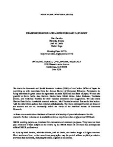
not reject the hypothesis that the pre-experimental estimates of teacher effects were unbiased. Thus, all of the specifications that conditioned on prior student test score in some manner yielded unbiased estimates of teacher effects. Fifth, in terms of being able to predict differences in student achievement at the end of the experimental year, the specifications using pre-experimental estimates based on student/peer controls and school fixed effects had the highest R2 – .226 for math and .169 in English language arts – while similar specifications without the school fixed effect were a close second. In other words, of the several specifications which we could not reject as being unbiased, the specifications with the lowest mean squared error in terms of predicting differences in student achievement were those which included student/peer controls. (Recall that the experimental design is also focused on measuring differences in student achievement within schools, so those too implicitly include school fixed effects.) To illustrate the predictive power of the pre-experimental estimates, we plotted the difference in student achievement within teacher pairs against the difference in preexperimental teacher effects for these preferred specifications in Figure 1 (math on the left, English language arts on the right), along with the estimated regression line and the prediction from a lowess regression. Teachers were ordered within the randomized pair so that the values on the x-axis are positive, representing the difference between the higher and lower value-added teacher. Thus, we expect the difference in achievement between the two classrooms to be positive, and more positive as the difference in valueadded increases between the two teachers. This pattern is quite apparent in the data, and

26

both the regression line and the lowess predictions lie near to the 45 degree line as expected. How much of the systematic variation in teacher effects are the imperfect measures capturing? Given that the experimental estimates themselves are based on a sample of students, one would not expect an R2 of 1 in Table 6 even if the value-added estimates were picking up 100 percent of the “true” variation in teacher effects. A quick back of the envelope calculation suggests that the estimates are picking up about half the variation in teacher effects. The total sum of squared differences (within each pair) in mean classroom performance in math was 17.6. Assuming that the teacher effects within each pair were uncorrelated, the total variation that we would have expected, even if we had teachers actual effects, μ1p0 and μ2p , would have been 7.48 (= 78 * 2 * .2192, where .219 is the s.d. of actual teacher effects from table 3). As a result, the maximum R2 we could have expected in a regression such as those in Table 6 would have been 7.48/17.6=.425. Thus, the variation in math teacher effects within pairs that we were able to explain with the value added estimates accounted for about 53 percent of the maximum (.226/.425). A similar calculation shows that value added estimates in English Language Arts also explained about 53 percent of the teacher level variation. Finally, the remaining columns of Table 6 report differences in student achievement one and two years after the experimental assignment to a particular teacher. After students have dispersed into other teachers’ classrooms in the year following the experiment, about half of the math impact had faded. (Each of the coefficients declines by roughly 50 percent.) In the second year after the experimental year, the coefficients on the teacher effects on math had declined further and were not statistically different

27

from zero. In other words, while the mean student assigned to a high “value-added” teacher seems to outperform similar students at the end of the year, the effects fade over the subsequent two years. As discussed in the conclusion, this has potentially important implications for calculating the cumulative impact of teacher quality on achievement.

Testing for Compensatory Teacher Assignment

If principals were to compensate a student for having been assigned a high- (or low-) value-added teacher one year with a low (or high-) value-added teacher the next year, we would be overstating the degree of fade-out in the specifications above. That is, a student randomly assigned a high-impact teacher during the experiment might have been assigned a low-impact teacher the year after. However, the (non-experimental) value-added estimates for the teacher a student was assigned in the experimental year and the teacher they were assigned the following year were essentially uncorrelated (-0.01 for both math and English language arts), suggesting this was not the mechanism. Another way to test this hypothesis is to re-estimate the relationships using student-level data and include fixed effects for teacher assignments in subsequent years (note that this strategy conditions on outcomes that occurred after random assignment, and therefore no longer relies solely on experimental identification due to random assignment). As reported in Table 7, there is little reason to believe that compensatory teacher assignments accounts for the fade-out. The first two columns report results from student-level regressions that were similar to the pair-level regression reported for first and second year scores in the previous table. The only difference from the corresponding estimates in Table 6 is that these estimates are estimated at the student level and,

28

therefore, place larger weight on classrooms with more students. As we would have expected, this reweighting resulted in estimates that were very similar to those reported in Table 6. The third column of Table 7 reports the coefficient on one’s experimental year teacher in predicting one’s subsequent performance, including fixed effects for one’s teacher in the subsequent year. Sample size falls somewhat in these regressions because we do not have reliable teacher assignments for a few students. If principals were assigning teachers in successive years to compensate (or to ensure that students have similar mean teacher quality over their stay in school), one would expect the coefficient on the experimental year teacher’s effect to rise once the teacher effects are added. The coefficient is little changed. The same is true in the second year after the experimental year. A Model for Estimating Fade-Out in the Non-Experimental Sample

In the model for estimating teacher effects in equation (1), we attached no interpretation to the coefficient on baseline student performance. The empirical value of the coefficient could reflect a range of factors, such as the quality or prior educational inputs, student sorting among classrooms based on their most recent performance, etc. However, in order to be able to compare the degree of fade-out observed following random assignment with that during the pre-experimental period, we need to introduce some additional structure. Suppose a student’s achievement were a sum of prior educational inputs, decaying at a constant annual rate, plus an effect for their current year teacher. We could then substitute the following equation for equation (1): Aijt = φijt + ε ijt , where φijt = δφijt −1 + μ jt + θ jt

29

In the above equation, φijt represents a cumulative school/teacher effect and δ represents the annual rate of persistence (or 1- annual rate of decay). As before, μ jt represents the effect of one’s current year teacher and θ jt a non-persistent classroom by year error term. By taking differences and re-arranging terms, we could rewrite the above as: Aijt = δAijt −1 + μ jt + θ jt + (ε ijt − δε ijt −1 ) OLS will yield biased estimates of δ, since Aijt −1 and ε ijt −1 will be correlated. As a result, we use a vector of indicators for teacher assignment in year t-1 as an instrument for Aijt −1 , in generating an IV estimator for δ.8 Table 8 reports the resulting estimates of δ using three different specifications, using fixed effects for the current-year teacher, including fixed effects for the current year classroom, and including controls for other student-level traits. Each of the estimates in the table suggest a large degree of fade-out of teacher effects in the non-experimental data, with between 50 and 60 percent of teacher and school impacts fading each year. Using the non-experimental estimate of δ, we constructed a test of the joint validity of our estimates of δ and of the teacher effects, μ j . To do so, we again studied differences in student achievement for randomly assigned classrooms of students, premultiplying our empirical Bayes estimate of the teacher effect by the fade-out parameter:

(

)

Y2 pt − Y1 pt = β δ tVA2 p − δ tVA1 p + ε~pt

The results for t=0, 1 and 2 are reported in Table 9. The estimates for years t=1 and 2 are quite imprecise. However, when pooling all three years, we could not reject the

8

In contemporaneous work, Jacob et al. (2008) has proposed a similar estimation method.

30

hypothesis that a one unit difference in pre-experimental impact estimates, adjusted for the degree of fade out between year 0 and year t, was associated with a comparable difference in student achievement following random assignment. In other words, nonexperimental estimates of teacher effects, combined with a non-experimental estimate of the amount of fadeout per year, are consistent with student achievement in both the year of the experiment and the two years following.

External Validity: Is Teacher-Student Sorting Different in Los Angeles?

Given the ubiquity of non-experimental impact evaluation in education, there is a desperate need to validate the implied causal effects with experimental data. In this paper, we have focused on measuring the extent of bias in non-experimental estimates of teacher effects in Los Angeles. However, there may be something idiosyncratic about the process by which students and teachers are matched in Los Angeles. For instance, given the large number of immigrant families in Los Angeles, parents may be less involved in advocating for specific teachers for their children than in other districts. Weaker parental involvement may result in less sorting on both observables and unobservables. To test whether the nature and extent of tracking of students to teachers in Los Angeles are different than in other districts, we calculated two different measures of sorting on observables in Los Angeles: the standard deviation in the mean baseline expected achievement (the prediction of end-of-year scores based on all of the student baseline characteristics) of students typically assigned to different teachers and the correlation between the estimated teacher effect and the baseline expected achievement of students. We estimated both of these statistics in a manner analogous to how we

31

estimate the variance in teacher effects in table 3, using the covariance between one year and the next to estimate the signal variance and covariance. This way, we are estimating the variance and correlation in the persistent component, in the same way that we estimate the variance of the persistent component in the teacher effect. We calculated these measures in three districts for which we were able to obtain data: New York City, Boston and Los Angeles. We further split out the experimental schools in Los Angeles to investigate whether teacher-student sorting in our experimental schools differed from Los Angeles in general. To achieve some comparability, we standardized the test scores in all three districts by grade and year and used similar sets of regressors to estimate the teacher effects. There are three striking findings reported in Table 10. First, the standard deviation in teacher effects is very similar in the three cities, ranging from .16 to .19 in math and .13 to .16 in English Language arts. Second the degree of sorting of students based on baseline expected achievement was similar in Los Angeles, NYC and Boston with a standard deviation in mean student baseline expected achievement of about .5. Third, the correlation between the teacher effect and the baseline expected achievement was similar in all three cities, but small: between .04 and .12. In other words, in all three cities, there is strong evidence of tracking of students based on baseline expected performance into different teachers’ classrooms. However, there is little correlation between students’ baseline achievement and the effectiveness of the teachers they were assigned. Nevertheless, when it comes to both types of sorting measured in Table 10, Los Angeles is not markedly different from Boston or NYC. Finally, on all of the

32

measures reported in Table 10, the schools participating in the experiment are similar to the other Los Angeles schools. The low correlation between students’ baseline achievement and the current year “teacher effect” has important implications, in light of the fade-out in teacher effects noted above. In the presence of such fade-out, a students’ teacher assignment in prior school years would play a role in current achievement gains – conditional on baseline performance, a student who had a particularly effective teacher during the prior year would under-perform relative to a student with a particularly ineffective teacher during the prior year. Indeed, Rothstein (2008) presents evidence of such a phenomenon using North Carolina data. However, to the extent that the prior teacher effect is only weakly correlated with the quality of one’s current teacher, excluding prior teacher assignments would result in little bias when estimating current teacher effects.

Conclusion

Our analysis suggests that standard teacher value-added models are able to generate unbiased and reasonably accurate predictions of the causal short-term impact of a teacher on student test scores. Teacher effects from models that controlled both for prior test scores and mean peer characteristics performed best, explaining over half of the variation in teacher impacts in the experiment. Since we only considered relatively simple specifications, this may be a lower bound in terms of the predictive power that could be achieved using a more complex specification (for example, controlling for prior teacher assignment or available test scores from earlier years). Although such additional controls may improve the precision of the estimates, we did not find that they were

33

needed to remove bias.9 While our results need to be replicated elsewhere, these findings from Los Angeles schools suggest that recent concerns about bias in teacher value added estimates may be overstated in practice. However, both our experimental and non-experimental analyses find significant fade-out of teacher effects from one year to the next, raising important concerns about whether unbiased estimates of the short-term teacher impact are misleading in terms of the long-term impacts of a teacher. Interestingly, it has become commonplace in the experimental literature to report fade-out of test score impacts, across a range of different types of educational interventions and contexts. For instance, experiments involving the random assignment of tutors in India (Banerjee et al., 2007) and recent experimental evaluations of incentive programs for teachers and students in developing countries (Glewwe, Ilias and Kremer, 2003) showed substantial rates of fade out in the first few years after treatment. In their review of the evidence emerging from the Tennessee class size experiment, Krueger and Whitmore (2001) conclude achievement gains one year after the program fell to between a quarter and a half of their original levels. In a recent re-analysis of teacher effects in the Tennessee experiment, Konstantopoulos (2007, 2008) reports a level of fade-out similar to that which we observed. McCaffrey et al. (2004), Jacob et al. (2008) and Rothstein (2008) also report considerable fade-out of estimated teacher effects in non-experimental data. However, it is not clear what should be made of such “fade out” effects. Obviously, it would be troubling if students are simply forgetting what they have learned, or if value-added measured something transitory (like teaching to the test) rather than true 9

Rothstein (2008) also found this to be the case, with the effect of one’s current teacher controlling for prior teacher or for earlier test scores being highly correlated (after adjusting for sampling variance) with the effect when those controls were dropped.

34

learning. This would imply that value added overstates long-term teacher effectiveness. However, this “fade out” evidence could also reflect changing content of the tests in later grades (students do not forget the content that they learned in prior years, it is no longer tested). Alternatively, the impact of a good teacher could spill over to other students in future years through peer effects making relative differences in test scores appear to shrink. These types of mechanisms could imply that short term value added measures are indeed accurate indicators of long-term teacher effectiveness, despite apparent fade out. Better understanding of the mechanism generating fade out is critically needed before concluding that teacher effects on student achievement are ephemeral.

35

References:

Aaronson, Daniel, Lisa Barrow and William Sander (2007) “Teachers and Student Achievement in Chicago Public High Schools” Journal of Labor Economics Vol. 24, No. 1, pp. 95-135. Andrabi, Tahir, Jishnu Das, Asim I. Khwaja, Tristan Zajonc (2008) “Do Value-Added Estimates Add Value? Accounting for Learning Dynamics” Harvard University unpublished working paper, Feb. 19. Armour, David. T. (1976). Analysis of the school preferred reading program in selected Los Angeles minority schools. R-2007-LAUSD. (Santa Monica, CA: Rand Corporation). Banerjee, A.V., S. Cole, E. Duflo and L. Linden, “Remedying Education: Evidence from Two Randomized Experiments in India,” Quarterly Journal of Economics, August 2007, Vol. 122, No. 3, Pages 1235-1264. Cantrell, S., J. Fullerton, T.J. Kane, and D.O. Staiger, “National Board Certification and Teacher Effectiveness: Evidence from a Random Assignment Experiment,” working paper, March 2007. Glewwe, P., N. Ilias, and M. Kremer, “Teacher Incentives,” NBER working paper #9671, May 2003. Gordon, Robert, Thomas J. Kane and Douglas O. Staiger, (2006) “Identifying Effective Teachers Using Performance on the Job” Hamilton Project Discussion Paper, Published by the Brookings Institution. Hanushek, Eric A. (1971). “Teacher characteristics and gains in student achievement; estimation using micro data”. American Economic Review, 61, 280-288. Jacob, Brian and Lars Lefgren (2005) “Principals as Agents: Student Performance Measurement in Education” NBER Working Paper No. 11463. Jacob, B.A., L. Lefgren, and D. Sims, “The Persistence of Teacher-Induced Learning Gains,” NBER working paper #14065, June 2008. Kane, Thomas J., Jonah Rockoff and Douglas Staiger, (Forthcoming) “What Does Certification Tell Us about Teacher Effectiveness?: Evidence from New York City” Economics of Education Review (Also NBER Working Paper No. 12155, April 2006. Konstantopoulos, S. “How Long Do Teacher Effects Persist?” IZA Discussion Paper No. 2893, June 2007.

36

Konstantopoulos, Spyros (2008) “Do Small Classes Reduce the Achievement Gap between Low and High Achievers? Evidence from Project STAR” The Elementary School Journal Vol 108, No. 4, pp. 278-291. McCaffrey, D.F. and L.S. Hamilton, “Value-Added Assessment in Practice,” RAND Technical Report, The RAND Corporation, Santa Monica, CA, 2007. McCaffrey, Daniel, J.R. Lockwood, Daniel Koretz and Laura Hamilton (2003) Evaluating Value-Added Models for Teacher Accountability, (Santa Monica, CA: Rand Corporation). McCaffrey, Daniel F., J. R. Lockwood, Daniel Koretz, Thomas A. Louis, Laura Hamilton (2004) “Models for Value-Added Modeling of Teacher Effects” Journal of Educational and Behavioral Statistics, Vol. 29, No. 1, Value-Added Assessment Special Issue., Spring, pp. 67-101. Morris ,Carl N (1983) “Parametric Empirical Bayes Inference: Theory and Applications” Journal of the American Statistical Association, 78:47-55. Murnane, R. J. & Phillips, B. R. (1981). “What do effective teachers of inner-city children have in common?” Social Science Research, 10, 83-100. Nye, Barbara, Larry Hedges and Spyros Konstantopoulos (2004) “How large are teacher effects?” Educational Evaluation and Policy Analysis Volume 26, pp. 237-257. Raudenbush, Stephen W. (2004) “What Are Value-Added Models Estimating and What Does This Imply for Statistical Practice?” Journal of Educational and Behavioral Statistics, Vol. 29, No. 1, Value-Added Assessment.Special Issue. Spring, pp. 121-129. Raudenbush, Stephen W. and A.S. Bryk (2002), Hierarchical Linear Models: Applications and Data Analysis Methods, Newbury Park, CA: Sage Publications. Rivkin, Steven, Eric Hanushek and John Kain (2005) “Teachers, Schools and Academic Achievement” Econometrica Vol. 73, No. 2, pp. 417-458. Rockoff, Jonah E. (2004) “The Impact of Individual Teachers on Student Achievement: Evidence from Panel Data” American Economic Review Vol. 92, No. 2, pp. 247252. Rothstein, J., “Teacher Quality in Educational Production: Tracking, Decay, and Student Achievement,” Princeton University Working Paper, May 2008. Rubin, Donald B., Elizabeth A. Stuart; Elaine L. Zanutto (2004) “A Potential Outcomes View of Value-Added Assessment in Education” Journal of Educational and

37

Behavioral Statistics, Vol. 29, No. 1, Value-Added Assessment Special Issue, Spring, pp. 103-116. Sanders, William L. and June C. Rivers (1996) “Cumulative and Residual Effects of Teachers on Future Student Academic Achievement” Research Progress Report University of Tennessee Value-Added Research and Assessment Center. Todd, Petra E. and Kenneth I. Wolpin (2003) “On the Specification and Estimation of the Production Function for Cognitive Achievement” Economic Journal Vol. 113, No. 485.

38

Figure 1 Within Pair Differences in Pre-experimental Value-added and End of First Year Test Score

0

.4

.8

45-degree Line

1.2 .8 .4 0 -.4 -.8 0 .4 .8 W ithin Pair Differenc e in Pre-experimental Value-added p

W ithin Pair D ifferenc e in Pre-experi mental Value-added

Observed

-1.2

-.8

-.4

0

.4

.8

1.2

Within Pair Difference in Av erage End of Firs t Year Tes t Sc ore

English Language Arts

-1.2

Within Pair Difference in Average End of F irs t Year Tes t Sc ore

Mathematics

Linear Fitted V alues

O bserv ed Lowess Fitted Values 45-degree Line 1

Observed

Linear Fitted Values

Li near F itted Values 45-degree Line Lowess Fitted Values Lowess F itt ed V al ues

Table 1: Sample Comparison - Teachers Experimental School Non-experimental Experimental Sample Sample

Non-experimental School Non-experimental Sample

Mean Teacher Effect in Math S.D. Mean Teacher Effect in ELA S.D.

-0.005 0.193 -0.007 0.150

-0.002 0.199 0.004 0.150

0.005 0.200 0.003 0.150

Black, Non-Hispanic Hispanic White, Non-Hispanic Other, Non-Hispanic Teacher Race/Ethnicity Missing

0.174 0.225 0.486 0.116 0.000

0.138 0.311 0.447 0.102 0.003

0.123 0.325 0.425 0.123 0.003

Years of Experience

15.648

10.542

10.758

140

1,785

11,352

N:

Note: Descriptive statistics based on the experimental years (2003-04 and 2004-05). The mean teacher effect in math and ELA were estimated using the full sample of schools and teachers, controlling for baseline scores, student characteristics, and peer controls.

Table 2: Sample Comparison - Students Experimental School Non-experimental Experimental Sample Sample

Non-experimental School Non-experimental Sample

Math Scores 2004 Mean S.D. 2005 Mean S.D. 2006 Mean S.D. 2007 Mean S.D.

0.027 0.931 -0.008 0.936 0.001 0.960 -0.016 0.956

-0.110 0.941 -0.113 0.940 -0.100 0.941 -0.092 0.941

0.024 1.008 0.028 1.007 0.037 1.006 0.030 1.006

ELA Scores 2004 Mean S.D. 2005 Mean S.D. 2006 Mean S.D. 2007 Mean S.D.

0.038 0.913 0.009 0.920 0.039 0.923 0.018 0.940

-0.113 0.936 -0.117 0.930 -0.096 0.928 -0.095 0.936

0.023 1.008 0.027 1.009 0.037 1.001 0.037 1.000

Black, Non-Hispanic Hispanic White, Non-Hispanic Other, Non-Hispanic

0.112 0.768 0.077 0.044

0.115 0.779 0.060 0.046

0.113 0.734 0.088 0.066

Grade 2 Grade 3 Grade 4 Grade 5

0.377 0.336 0.113 0.131

0.280 0.201 0.215 0.305

0.288 0.207 0.211 0.294

N:

3,554

43,766

273,525

Note: Descriptive statistics based on the experimental years (2003-04 and 2004-05). Students present both years are counted only once.

Table 3: Non-experimental Estimates of Teacher Effect Variance Components Standard Deviation of Each Component (in Student-level Standard Deviation Units)

Specification Used for Non-experimental Teacher Effect

Teacher Effects

Teacher by Mean Sample Year Random Size per Effect Teacher

Math Levels with... No Controls Student/Peer Controls (incl. prior scores) Student/Peer Controls (incl. prior scores) & School F.E. Student Fixed Effects

0.448 0.231 0.219 0.101

0.229 0.179 0.177 0.061

47.255 41.611 41.611 47.255

Math Gains with... No Controls Student/Peer Controls Student/Peer Controls & School F.E.

0.236 0.234 0.225

0.219 0.219 0.219

43.888 43.888 43.888

English Language Arts Levels with... No Controls Student/Peer Controls (incl. prior scores) Student/Peer Controls (incl. prior scores) & School F.E. Student Fixed Effects

0.453 0.184 0.175 0.084

0.224 0.171 0.170 0.027

47.040 41.504 41.504 47.040

English Language Arts Gains with... No Controls Student/Peer Controls Student/Peer Controls & School F.E.

0.192 0.183 0.177

0.203 0.203 0.203

43.103 43.103 43.103

Note: The above estimates are based on the total variance in estimated teacher fixed effects using observations from the pre-experimental data (years 1999-2000 through 2002-03). See the text for discussion of the estimation of the decomposition into teacher by year random effects, student-level error, and "actual" teacher effects. The sample was limited to schools with teachers in the experimental sample. Any individual students who were in the experiment were dropped from the pre-experimental estimation, to avoid any spurious relationship due to regression to the mean, etc.

Table 4. Regression of Experimental Difference in Student Baseline Characteristics on Non-Experimental Estimates of Differences in Teacher Effect

Baseline Scores

Baseline Demographics & Program Participation

Gifted Language and Ever Special Score Talented Retained Education Hispanic

Specification Used for Non-experimental Teacher Effect

Math Score

Math Levels with Student/Peer Controls

-0.109 (0.225) 44

0.027 (0.267) 44

-0.013 (0.022) 78

-0.048 (0.038) 78

-0.042 (0.033) 78

0.043 (0.340) 44

0.282 (0.381) 44

0.021 (0.031) 78

-0.049 (0.049) 78

-0.053 (0.053) 78

N: ELA Levels with Student/Peer Controls N:

English Language Status

Black

Title I

Free Lunch

Level 1 to 3

-0.043 (0.043) 78

-0.002 (0.041) 78

0.041 (0.052) 78

0.032 (0.061) 78

-0.021 (0.070) 78

-0.021 (0.097) 78

-0.018 (0.058) 78

0.106 (0.082) 78

0.082 (0.084) 78

-0.071 (0.123) 78

Note: Each baseline characteristic listed in the columns was used as a dependent variable, regressing the within-pair difference in mean baseline characteristic on different non-experimental estimates of teacher effects. The coefficients were estimated in separate bivariate regressions with no constant. Robust standard errors are reported in parentheses. Baseline math and language arts scores were missing for the pairs that were in second grade.

Table 5. Regression of Experimental Difference in Rates of Attrition and Classroom Switching on Non-Experimental Estimates of Differences in Teacher Effect Specification Used for Non-experimental Teacher Effect Math Levels with Student/Peer Controls N: ELA Levels with Student/Peer Controls N:

Missing Test Score First Year

Second Year

Third Year

Switched Teacher

-0.008 (0.048) 78

0.019 (0.057) 78

-0.021 (0.058) 78

-0.036 (0.132) 78

-0.054 (0.072) 78

-0.015 (0.081) 78

0.034 (0.098) 78

-0.153 (0.164) 78

Note: Each baseline characteristic listed in the columns was used as a dependent variable, regressing the within-pair difference in rates of missing test score or switching on different non-experimental estimates of teacher effects. The coefficients were estimated in separate bivariate regressions with no constant. Robust standard errors are reported in parentheses.

Table 6. Regression of Experimental Difference in Average Test Scores on Non-Experimental Estimates of Differences in Teacher Effect

Specification Used for Non-experimental Teacher Effect Math Levels with... No Controls Student/Peer Controls (incl. prior scores) Student/Peer Controls (incl. prior scores) & School F.E. Student Fixed Effects

Math Gains with... No Controls Student/Peer Controls Student/Peer Controls & School F.E.

English Language Arts Levels with... No Controls Student/Peer Controls (incl. prior scores) Student/Peer Controls (incl. prior scores) & School F.E. Student Fixed Effects

English Language Arts Gains with... No Controls Student/Peer Controls Student/Peer Controls & School F.E.

N:

Test Score First Year Coefficient R2

0.511*** (0.108) 0.852*** (0.177) 0.905*** (0.180) 1.859*** (0.470)

0.185

0.794*** (0.201) 0.828*** (0.207) 0.865*** (0.213)

0.162

0.418** (0.155) 0.987*** (0.277) 1.089*** (0.289) 2.144*** (0.635)

0.103

0.765** (0.242) 0.826** (0.262) 0.886** (0.274) 78

0.210 0.226 0.153

0.171 0.177

0.150 0.169 0.116

0.100 0.108 0.115

Test Score Test Score Second Year Third Year Coefficient Coefficient

0.282** (0.107) 0.359* (0.172) 0.390* (0.176) 0.822 (0.445)

0.124 (0.101) 0.034 (0.133) 0.07 (0.136) 0.304 (0.408)

0.342 (0.185) 0.356 (0.191) 0.382 (0.200)

0.007 (0.146) 0.01 (0.151) 0.025 (0.157)

0.323 (0.173) 0.477 (0.284) 0.569 (0.307) 1.306 (0.784)

0.255 (0.157) 0.476 (0.248) 0.541* (0.264) 1.291* (0.642)

0.198 (0.243) 0.276 (0.261) 0.311 (0.278)

0.258 (0.228) 0.321 (0.241) 0.346 (0.253)

78

78

Note: Each baseline characteristic listed in the columns was used as a dependent variable (math or ELA scores, corresponding to the teacher effect), regressing the within-pair difference in mean test scores on different non-experimental estimates of teacher effects. The coefficients were estimated in separate bivariate regressions with no constant. Robust standard errors are reported in parentheses.

Table 7: Student-Level Regressions of Student Test Scores On Non-Experimental Estimates of Teacher Effect Specification Used for Non-experimental Teacher Effect Math Levels with Student/Peer Controls N: ELA Levels with Student/Peer Controls N: Student-Level Controls Second Year Teacher F.E. Second x Third Year Teacher F.E.

First Year Score

Second Year Score

Third Year Score

0.830*** (0.180) 2,905

0.401* (0.177) 2,685

0.391* (0.189) 2,656

0.047 (0.142) 2,504

0.016 (0.294) 2,489

1.064*** (0.289) 2,903

0.565* (0.287) 2,691

0.681* (0.282) 2,665

0.554* (0.255) 2,503

0.606 (0.372) 2,488

No

No Yes

No

No

No

Yes

Note: The above were estimated with student-level regressions using fixed effects for each experimental teacher pair. The dependent variable was the student's math score for the first row of estimates, and the student's ELA score for the second row of estimates. Robust standard errors (in parentheses) allow for clustering at the teacher-pair level.

Table 8: IV Estimates of Teacher Effect Fade-out Coefficient A Math N: English Language Arts N: Current Teacher F.E. Current Classroom F.E. Student Controls

B

C

0.489*** (0.006) 89,277

0.478*** (0.006) 89,277

0.401*** (0.007) 89,277

0.533*** (0.007) 87,798

0.514*** (0.007) 87,798

0.413*** (0.009) 87,798

Yes No No

No Yes No

No Yes Yes

Note: The table reports coefficients on baseline score, estimated using separate 2SLS regressions with student test score as the dependent variable. Each specification included controls as indicated and grade-by-year fixed effects. Baseline test score is instrumented using a teacher dummy variable for the teacher associated with the baseline test.

Table 9. Regression of Experimental Difference in Average Test Scores on Non-Experimental Estimates of Differences in Teacher Effect Adjusted for Fade Out in Years 1 and 2

Specification Used for Non-experimental Teacher Effect

P-value for Test of Coefficients Years 0, 1, and Equivalent Across 2 Pooled Years

Year 0

Year 1

Year 2

Math Levels with Student/Peer Controls

0.852*** (0.177)

0.894* (0.429)

0.209 (0.826)

0.843*** (0.207)

0.311

Math Gains with Student/Peer Controls

0.828*** (0.207)

0.889 (0.477)

0.060 (0.941)

0.819*** (0.239)

0.289

ELA Levels with Student/Peer Controls

0.987*** (0.277)

1.155 (0.689)

2.788 (1.454)

1.054** (0.343)

0.144

ELA Gains with Student/Peer Controls

0.826** (0.262)

0.668 (0.631)

1.880 (1.413)

0.829** (0.319)

0.170

78

78

N:

78

234

Note: Each year's classroom average test score was used as the dependent variable, regressing the within-pair difference in average test score on different non-experimental estimates of teacher effects discounted in year 1 by the coefficients in column "C" of Table 8 and in year 2 by the square of those same coefficients. The coefficients were estimated in separate regressions with no constant. Robust standard errors are reported in parentheses.

Table 10: Comparing Assortive Matching in Los Angeles to Other Urban Districts Experimental Schools in All Schools in Los All Schools in New Los Angeles Angeles York City Math ELA Math ELA Math ELA

All Schools in Boston Math ELA

Standard Deviation in Teacher Effect

0.184

0.135

0.189

0.139

0.157

0.121

0.191

0.162

Standard Deviation in Baseline Expected Achievement in Teacher's Classroom

0.400

0.408

0.493

0.487

0.512

0.513

0.528

0.539

Correlation between Teacher Effect and Baseline Expected Achievement in Teacher's Classroom

0.120

0.118

0.091

0.085

0.041

0.083

0.114

0.103

Note: Estimated using non-experimental samples of 4th and 5th graders in years 2000-2003 for Los Angeles, 2000-2006 for New York City, and 2006-2007 for Boston. Teacher value-added and baseline achievement estimated including student-level controls for baseline test scores, race/ethnicity, special ed, ELL, and free lunch status; classroom peer means of the student-level characteristics; and grade-by-year F.E.