IEICE TRANS. COMMUN., VOL.E89–B, NO.3 MARCH 2006
1033
LETTER
New Formula of the Polarization Entropy Jian YANG† , Yilun CHEN† , Yingning PENG† , Nonmembers, Yoshio YAMAGUCHI†† , and Hiroyoshi YAMADA†† , Members
SUMMARY In this Letter, a new formula is proposed for calculating the polarization entropy, based on the least square method. In the proposed formula, there is no need to calculate the eigenvalues of a covariance matrix as well as to use logarithm. So the computing time on the polarization entropy is reduced. Using polarimetric SAR data, the authors validate the effectiveness of the new formula. key words: polarization, Synthetic Aperture Radar (SAR), remote sensing
1.
Introduction
In polarimetric radar remote sensing, the polarization entropy is one of important parameters for target classification, target detection and so on [1]–[6]. For calculating the polarization entropy, however, one has to obtain the eigenvalues of a covariance matrix and then use logarithm. Consequently, some computation cost is necessary when we need to obtain all the entropy values of windows of interest in a polarimetric SAR image. In general, there may be more than one million pixels in a SAR image. So it is important to propose a simple method to calculate the polarization entropy. This paper will solve this problem. 2.
The polarization entropy
The entropy is originally used to describe the chaos extent in nature. Later, it was introduced to radar polarimetry [1]–[3]. Consider the following polarimetric covariance matrix [C] = (ci j )3×3
(1)
a0 = c11 c23 c32 + c13 c22 c31 + c12 c21 c33 −c11 c22 c33 − c12 c23 c31 − c13 c21 c32 a1 = c11 c22 + c22 c33 + c33 c11 −c12 c21 − c23 c32 − c31 c13 a2 = −c11 − c22 − c33
H=−
3 X
ki log3 ki
or equivalently λ3 + a2 λ2 + a1 λ + a0 = 0
(3)
where Manuscript received June 20, 2005. Manuscript revised August 25, 2005. † Dept. of Electronic Engineering, Tsinghua University Beijing 100084 China †† Dept. of Information Engineering Niigata University, 8050, Niigata-shi, 950-2181, Japan
(7)
i=1
where ki = P3λi j=1
λj
.
For target classification or target detection in a polarimetric SAR image, we need to obtain more than one million entropy values in general. Consequently, some computation cost is necessary. So it is important to propose a simple method to calculate the polarization entropy. 3.
The new formula
Consider that let p(x) = b0 +b1 x+b2 x2 +b3 x3 +b4 x4 approximate −x log3 x. Since −x log3 x equals zeros when x = 0 or x = 1, we assume that p(0) = 0 and p(1) = 0. It leads to b0 = 0 and b4 = −b1 − b2 − b3 . So it is reasonable to let AH = b1 + b2
3 X
ki2 + b3
i=1
(2)
(5) (6)
Let λi (i = 1, 2, 3) be the three eigenvalues of the matrix [C] = (cij )3×3 . Then the polarization entropy is defined by
Its eigenvalues are obtained by [C] x = λ x
(4)
approximate H = −
3 X
ki3 − (b1 + b2 + b3 )
i=1 3 P i=1
3 X
ki4
i=1
ki log3 ki . Use the least square
method, i.e., ZZ 2 min (H − AH) dk1 dk2
(8)
Ω
where Ω is the area determined by k1 − k2 ≥ 0, k1 + 2k2 − 1 ≥ 0 and 1 − k1 − k2 ≥ 0, shown in Figure 1. Letting ZZ ∂ 2 (H − AH) dk1 dk2 = 0 (9) ∂bi Ω we obtain
IEICE TRANS. COMMUN., VOL.E89–B, NO.3 MARCH 2006
1034
Fig. 1
The area Ω for the least square method
AH = 2.3506 − 5.7613
3 X
Fig. 2
The area Ω1 for the least square method
ki2 +
i=1
6.0611
3 X
ki3
i=1
Note that ki = P3λi j=1
λj
− 2.6504
3 X
[C] ki4
(10)
i=1
obtain
is derived from the eigenvalues
of the covariance matrix [C] = (ci j )3×3 , i.e., the roots of (1). According to Vieta’s Theorem which expresses the coefficients of a polynomial in terms of its roots [7], we derive the following formula from (10) AH = 3.9408
a1 a0 a2 + 7.5818 3 − 5.3008 14 2 a2 a2 a2
a 0 , a 1 , a 2 by(4)~(6)
t1 =
a1 a t 2 = 03 a 22 a2
(11)
where a0 , a1 and a2 are given by (4)-(6). Obviously, one may directly obtain the polarization entropy from (11) without solving an eigenvalue equation. On average, the corresponding absolute error is 0.006 in theory, i.e., Z 1 | H − AH| dk1 dk2 = 0.006 (12) |Ω|
t1 < 0.0481 t 2 < 0.0006 No
obtain
AH by(11)
Yes
obtain
AH by(13)
Ω
This demonstrates a good approximation by the proposed formula (11). However, if the maximum eigenvalue of the covariance matrix [C] is approximately equal to 1, the polarization entropy is very small and the relative error by (10) is a little large although the absolute error is very small. When k1 ≥ γ = 0.95, we can prove that a0 ≤ 0.0006 a32 and a1 ≤ 0.0481 a22 . For this case, the following formula of the polarization entropy is derived, based on the least square method over a small area Ω1 as shown in Figure 2: AH = 5.2819
a1 a0 a21 + 54.8584 − 35.6980 a22 a32 a42
(13)
if aa12 ≤ 0.0481 and aa03 ≤ 0.0006. We also let γ be several 2 2 other constants for calculating the polarization entropy
Fig. 3
The procedure for calculating the polarization entropy
by using the NASA/JPL AIRSAR L-band data of San Francisco, but the corresponding calculation accuracy of the proposed approach is worse than that when γ = 0.95. So we select γ = 0.95 in this letter. When we calculate the polarization entropy by the proposed formula, it is better to get t1 = aa21 and t2 = aa03 2 2 first. After comparing t1 and t2 with 0.0481 and 0.0006, a2 respectively, we submit t1 = aa21 , t2 = aa30 and t21 = a14 2 2 2 into (11) or (13) to obtain the entropy. In this way, the computation cost is reduced. Figure 3 shows the procedure for calculating the polarization entropy.
LETTER
1035
University. References
Fig. 4
The procedure for calculating the polarization entropy
Table 1
Comparison of calculation results by two formulae
sea area park area urban area whole area
4.
Av. value of H 0.058 0.607 0.459 0.360
Av. value of AH 0.055 0.607 0.473 0.365
Av. absolute error 0.003 0.006 0.016 0.008
Calculation result and conclusion
To validate the effectiveness of the proposed formula, we used a NASA/JPL AIRSAR L-band image of San Francisco (700 by 900 pixels). As shown in Figure 4, we selected three areas consisting of a sea area, a park area and an urban area. For each pixel, the entropy of an adjacent 3 by 3 window was calculated by (7) and (11) or (13). The calculation results are given in Table 1, validating a good approximation by the proposed formula. In addition, we calculated the polarization entropy of the whole area by C programming language. Except the computation time on covariance matrices, the running time for obtaining the entropy by the proposed formula was about 9 seconds by a P4 computer (2.0GHz 256MRAM ), whereas it took about 195 seconds when the formula (7) was used, demonstrating the efficiency of the proposed formula. Acknowledgments This work was supported by the National Natural Science Foundation of China (40271077), by the National Important Fundamental Research Plan of China (2001CB309401), by the Science Foundation of National Defence of China, by the Research Fund for the Doctoral Program of Higher Education of China, by the Aerospace Technology Foundation of China, and by the Fundamental Research Foundation of Tsinghua
[1] S. R. Cloude, E. Pottier, ”A review of target decomposition theorems in radar polarimetry”, IEEE Trans. Geosci. and Remote Sensing, vol.34, no.2, pp 498-518, 1996 [2] S. R. Cloude, and E. Pottier, ”An Entropy based classification scheme for land applications of polarimetric SAR”, IEEE Trans. Geosci. Remote Sensing, vol.35, no.1, pp. 6878, 1997. [3] Y.-Q. Jin, and S. R. Cloude, ”Numerical eigenanalysis of the coherency matrix for a layer of random nonspherical scatterers”, IEEE Trans. Geosci. Remote Sensing, vol.32, no.6, 1179-1185, 1994. [4] R. Touzi, F. Charbonneau, R. K. Hawkins, et al., ”Shipsea contrast optimization when using polarimetric SARs”, IEEE IGARSS, vol.1, pp.426- 428, 2001. [5] L. Ferro-Famil, E. Pottier and J.-S. Lee, ”Unsupervised classification of multifrequency and fully polarimetric SAR images based on the H/A Alpha - Wishart classifier”, IEEE Trans. Geosci. and Remote Sensing, vol.39, no.11, pp. 23322342, 2001. [6] J. Yang, G.. W. Dong, Y. N. Peng, Y. Yamaguchi, Y. Yamada, ”Generalized optimization of polarimetric contrast enhancement”, IEEE Geosci. Remote Sensing Lett., vol.1, no.3, pp.171-174, 2004. [7] Borwein, P. and Erdlyi, T. ”Newton’s Identities.” §1.1.E.2 in Polynomials and Polynomial Inequalities, New York: Springer-Verlag, pp.5-6, 1995.