New Technologies and the Labor Market Enghin Atalay Phai Phongthiengtham Sebastian Sotelo Daniel Tannenbaum∗ March, 2018
Abstract Using newspaper job ad text from 1960 to 2000, we measure job tasks and the adoption of individual information and communication technologies (ICTs). Most new technologies are associated with an increase in nonroutine analytic tasks, and a decrease in nonroutine interactive, routine cognitive, and routine manual tasks. We embed these interactions in a quantitative model of worker sorting across occupations and technology adoption. Through the lens of the model, the arrival of ICTs broadly shifts workers away from routine tasks, which increases the college premium. A notable exception is the Microsoft Office Suite, which has the opposite set of effects. JEL Codes: J24, M51, O33
∗
Atalay and Phongthiengtham: Department of Economics, University of Wisconsin-Madison. Sotelo: Department of Economics, University of Michigan-Ann Arbor. Tannenbaum: Department of Economics, University of Nebraska-Lincoln. We thank the participants of the Carnegie-Rochester-NYU Conference for helpful comments and Erin Robertson for excellent editorial assistance. We especially thank Brad Hershbein for his thoughtful and constructive discussion of our paper. We acknowledge financial support from the Washington Center for Equitable Growth.
1
1
Introduction
Enabled by increasingly powerful computers and the proliferation of new, ever more capable software, the fraction of workers’ time spent using information and communication technologies (ICTs) has increased considerably over the last half century.1 In this project, we quantify the impact of 48 individual and recognizable ICTs on the aggregate demand for routine and nonroutine tasks, on the allocation of workers across occupations, and on earnings inequality. We start by constructing a data set tracking the adoption rates of 48 ICTs across occupations and years. We assemble this data set through a text analysis of 4.2 million job vacancy ads appearing between 1960 and 2000 in the Boston Globe, New York Times, and Wall Street Journal.2 We extract information about jobs’ ICT use and task content, as measured by their appearance in the text of job postings. We study a wide set of technologies, ranging from office software (including Lotus 123, Word Perfect, Microsoft Word, Excel, and PowerPoint), enterprise programming languages (Electronic Data Processing and Sybase), general-purpose programming languages (COBOL, FORTRAN, and Java), to hardware (UNIVAC, IBM 360, and IBM 370), among others. With this data set, we document rich interactions between individual ICTs and the task content of individual occupations. One of the strengths of the data is that we observe ICT adoption separately by technology type, and indeed we find substantial heterogeneity in the impact of individual ICTs. We show that, for the most part, job ads that mention a new technology tend to also mention nonroutine analytic tasks more frequently, while mentioning other tasks less frequently.3 An important exception is office software, which, compared to other technologies, is relatively less likely to appear alongside words associated with nonroutine analytic tasks. Since our data set includes a wide range of occupations and technologies, we can speak directly to the macroeconomic implications of changes in the availability of ICTs while maintaining a detailed analysis of individual occupations. Informed by our micro estimates on the relationship between the tasks that workers perform and the technologies they use on 1
Nordhaus (2007) estimates that, between 1960 and 1999, the total cost of a standardized set of computations fell by between 30 and 75 percent annually, a rapid rate of change that far outpaced earlier periods. 2
We introduce part of this data set in an earlier paper, namely the measurement of job tasks and the mapping between job titles and SOCs (Atalay, Phongthiengtham, Sotelo, and Tannenbaum, 2017). In Atalay, Phongthiengtham, Sotelo, and Tannenbaum (2017), we use the text of job vacancy ads to explore trends in the task content of occupations over the second half of the 20th century, showing that withinoccupation changes in the tasks workers perform are at least as large as the changes that happen between occupations. We extract information about job-specific technology adoption to build on this earlier data set. 3
Building on a mapping between survey question titles and task categories introduced by Spitz-Oener (2006), we have identified words that represent nonroutine (analytic, interactive, and manual) and routine (cognitive and manual) tasks.
2
the job, we build a quantitative model of occupational sorting and technology adoption. In the model, workers sort into occupations based on their comparative advantage. They also choose which ICT to adopt, if any, based on the price of each piece of technology and the technology’s complementarity with the tasks involved in their occupation. Within the model, the availability of a new technology — which we model as a decline in the technology’s price — alters the types of tasks workers perform in their occupation. To explore the implications of new technologies on the labor market, we consider three sets of counterfactual exercises. These exercises investigate the effects of three groups of technologies: (i) Unix, (ii) the Microsoft Office Suite (Microsoft Excel, Microsoft PowerPoint, and Microsoft Word), and (iii) all 48 of the technologies in our sample. In each of the counterfactual exercises, we quantify the impact of the new technologies on occupations’ overall task content, workers’ sorting across occupations, and economy-wide income inequality. One of our main findings is that new technologies result in an increase in occupations’ nonroutine analytic task content, relative to other tasks. As we have documented elsewhere (Atalay, Phongthiengtham, Sotelo, and Tannenbaum, 2017) and confirm again here, workers with observable characteristics indicating high skill levels (i.e., highly educated workers) have a comparative advantage in producing nonroutine analytic tasks. Because new technologies increase the demand for nonroutine analytic tasks, the introduction of ICTs has (for the most part) led to an increase in income inequality. Overall, in a counterfactual economy in which our ICT technologies were never introduced, earnings would have been 15 log points lower for the average worker, and the college-high school skill premium would have been 4.0 log points lower.4 Unlike most other technologies in our data, Microsoft Office technologies are only weakly correlated with nonroutine analytic tasks, and are positively correlated with nonroutine interactive tasks. As a result, we find that the introduction of Microsoft Office software has decreased the skill premium, the gender gap, and income inequality, although the magnitude of these effects is small. Individual technologies whose use is concentrated in a few high-earning occupations, such as Unix, tend to modestly increase inequality. This paper relates to a rich literature exploring the implications of technological change for skill prices and the wage distribution (Katz and Murphy, 1992; Juhn, Murphy, and Pierce, 1993; Berman, Bound, and Machin, 1998; Krusell, Ohanian, Rios-Rull, and Violante, 2000). More recent work has argued that information technology complements high-skilled workers performing abstract tasks and substitutes for middle-skilled workers performing routine tasks (Autor, Levy, and Murnane, 2003; Goos and Manning, 2007; Autor, Katz, and Kearney, 2005; Acemoglu and Autor, 2011). Researchers have also studied the implications of changes in the demand for tasks on the male-female wage gap and the female share of employment 4
Between 1960 and 2000, the college-high school skill premium increased by 23 log points.
3
in high-wage occupations (Black and Spitz-Oener, 2010; Cortes, Jaimovich, and Siu, 2018). Our paper contributes to this literature by studying how new technologies complement (or substitute for) the types of tasks that workers of different skill groups perform. We find that ICTs tend to substitute for routine tasks (especially routine manual tasks) which are disproportionately performed by low skill workers. ICTs also allow high skill workers to focus on the activities in which they are most productive, which in our model is the essence of the complementarity between tasks and technologies. A key contribution of this paper is that we measure both technological adoption and the task content of occupations directly, over a period of immense technological change. Our paper relates to a second literature that directly measures the adoption of specific technologies and its effect on wages and the demand for skills. These include studies of the effect of computer adoption (Krueger, 1993; Entorf and Kramarz, 1998; Autor, Katz, and Krueger, 1998; Haisken-DeNew and Schmidt, 1999) or the introduction of broadband internet (Brynjolfsson and Hitt, 2003; Akerman, Gaarder, and Mogstad, 2015) on worker productivity and wages.5 Also exploiting text descriptions of occupations, Michaels, Rauch, and Redding (2016) provide evidence that, since 1880, new technologies that enhance human interaction have reshaped the spatial distribution of economic activity. Focusing on a more recent technological revolution, Burstein, Morales, and Vogel (2015) document how the diffusion of computing technologies has contributed to the rise of inequality in the U.S. Our paper builds on this literature by introducing a rich data set measuring the adoption of ICTs at the job vacancy level. The rest of the paper is organized as follows. Section 2 of the paper introduces our new data set. Section 3 provides direct evidence on the interaction between individual ICT adoption and task contents. Section 4 takes our micro estimates and uses a quantitative model to study the aggregate impact of ICTs, while Section 5 assesses three extensions of the model. Section 6 concludes.
2
A New Data Set Measuring ICT Adoption
The construction of this new data set builds on our previous work with newspaper help wanted ads (Atalay, Phongthiengtham, Sotelo, and Tannenbaum, 2017). In that paper, we show how to transform the text of help wanted ads into time-varying measures of the task content of occupations. In this paper, we turn to previously unexamined ad content: 5
Additional investigations of technology-driven reorganizations within specific firms or industries include Levy and Murnane (1996)’s study of a U.S. bank and Bartel, Ichniowski, and Shaw (2007)’s study of the steel valve industry.
4
mentions of ICTs. Our main data set is built from the universe of job vacancies published in three major metropolitan newspapers — the Boston Globe, New York Times, and Wall Street Journal — which we purchased from ProQuest. We use the text contained in each vacancy to measure the tasks that will be performed on the job, as well as to examine the computer and information technologies that will be used on the job. Our sample period spans 1960 to 2000. The original newspapers were digitized by ProQuest using an Optical Character Recognition (OCR) technology. We briefly describe the steps we take to transform this digitized text into a structured database. To begin, the raw text does not distinguish between job ads and other types of advertisements. Hence, in the first step, we apply a machine learning algorithm to determine which pages of advertisements are job ads. The top panel of Figure 1 presents a portion of a page that, according to our algorithm, contains job ads. This snippet of text refers to three job ads: first for a Software Engineer position, then a Senior Systems Engineer position, and finally for a second Software Engineer position. Within this page of ads, we then determine the boundaries of each individual advertisement (for instance, where the first Software Engineer ad ends and the Senior Systems Engineer ad begins) and the job title. In the second step we extract, from each advertisement, words that refer to tasks the new hire is expected to perform and technologies that will be used in the job. So that we may link our text-based data to occupation-level variables in the decennial census, including wages, education, and demographics, our procedure also finds the SOC code corresponding to each job title (for example, 151132 for the “Software Engineers” job title.)6 We extract job tasks from the text using a mapping between words and task categories based on Spitz-Oener (2006). The five tasks are nonroutine analytic, nonroutine interactive, nonroutine manual, routine cognitive, and routine analytic.7 Because we do not want our analysis to be sensitive to trends in word usage or meaning, we adopt a machine-learning 6
For additional details on the steps mentioned here, see Atalay, Phongthiengtham, Sotelo, and Tannenbaum (2017). In that paper we also address issues regarding the representativeness of newspaper ads, and the validity of task measures extracted from the text. Our data set, including information on occupations’ task and technology mentions is available at http://ssc.wisc.edu/˜eatalay/occupation data . There, we also provide the full list of words and phrases we associate with each task and technology. 7
We use the mapping of words to tasks as described in Atalay, Phongthiengtham, Sotelo, and Tannenbaum (2017). For convenience, we list the taxonomy again here: 1) nonroutine analytic: analyze, analyzing, design, designing, devising rule, evaluate, evaluating, interpreting rule, plan, planning, research, researching, sketch, sketching; 2) nonroutine interactive: advertise, advertising, advise, advising, buying, coordinate, coordinating, entertain, entertaining, lobby, lobbying, managing, negotiate, negotiating, organize, organizing, presentation, presentations, presenting, purchase, sell, selling, teaching; 3) nonroutine manual: accommodate, accommodating, accommodation, renovate, renovating, repair, repairing, restore, restoring, serving; 4) routine cognitive: bookkeeping, calculate, calculating, correcting, corrections, measurement, measuring; 5) routine manual: control, controlling, equip, equipment, equipping, operate, operating.
5
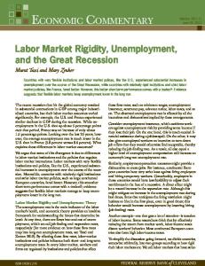
Figure 1: Text from the New York Times, January 12, 1997, Display Ad #87 SOFiWARE ENGINEERS - Modal Software Develop air-to-surface modal software, including design, code, unit test, integration and test, and documentation. Requires 5+ years software engineering experience with a BSEE/CS or Computer Engineering. Software development for real-time, multi-tasking/multi-processor, embedded systems experience a must. 3+ years C programming experience in a Unix environment and familiarity with modern software design methodologies essential. Knowledge of radar design principles a plus. Joint STARS The premiere ground surveillance system far the U.S. and allied forces. The DoD has authorized the full production of Joint STARS. In addition, significant activity on Joint STARS upgrades is underway. SENIOR SYSTEMS ENGINEERS Design and develop advanced, high-resolution radar imaging systems, including ultra-high resolution SAR and Moving Target Imaging Systems in real-time or near real-time environments. Represent the engineering organization ta senior technical management, potential partners and customers in industry and government; plan/coordinate R&D program activities; lead a team of hardware/soare/systems engineers; develop and test complex signal processing modes and algorithms in a workstation environment; support development with analyses, reports, documentation and technical guidance. Requires an MS or PhD in Engineering, Physics or Mathematics with experience in specification, Imaging anss and testing of Advanced Coherent Radar High-Resolution Must have strong math, physics and signal processing skills, C/C++ and ,AN programming expertise, plus familiarity with workstations and analytical tools such as The following require knowledge oF emulators, debuggers, and logic ana/. Knowledge of Ada, Unix, VxWorks, DigitalAlpha Processor and assembly language desirable. Radar systems experience plus. SOFTWARE ENGINEERS Define requirements and develop software far RCU or Intel microprocessor-based RSEs. Help define software requirements far LRU ECPs and the Contractor Logistics software program, including design, code, integration and test, and documentation. BSCS/EE preferred with 3-5 years real-time software development experience using Ada and/or FORTRAN programming languages. U IS- * SOFiWARE
engineers|- modal software develop air-to-surface modal software , including design , code , unit test , integration and test , and documentation . requires 5+ years software engineering experience with a b see cs or computer engineering . software development for real-time , multitasking multiprocessor , embedded systems experience a must . 3+ years c programming experience in a UNIX environment and familiarity with modern software design methodologies essential . knowledge of radar design principles a plus . joint stars the premiere ground surveillance system far the u . s . and allied forces . the DOD has authorized the full production of joint stars . in addition , significant activity on joint stars upgrades is underway . senior systems engineer| design and develop advanced , high-resolution radar imaging systems , including ultra-high resolution sear and moving target imaging systems in real-time or near realtime environments . represent the engineering organization ta senior technical management , potential partners and customers in industry and government ; plan coordinate r ; d program activities ; lead a team of hardware soared systems engineers ; develop and test complex signal processing modes and algorithms in a workstation environment ; support development with analysis , reports , documentation and technical guidance . requires an ms or PhD in engineering , physics or mathematics with experience in specification , imaging ans and testing of advanced coherent radar high-resolution must have strong math , physics and signal processing skills , c c and , an programming expertise , plus familiarity with workstations and analytical tools such as the following require knowledge of emulators , debuggers , and logic Ana . knowledge of Ada , UNIX , vxworks , digital alpha processor and assembly language desirable . radar systems experience plus. software engineers|define requirements and develop software far r cu or Intel microprocessorbased rs es . help define software requirements far lr u e cps and the contractor logistics software program , including design , code , integration and test , and documentation . bscs ee preferred with 3-5 years real-time software development experience using Ada and or FORTRAN programming languages . u is- software
Notes: The top panel presents text from three vacancy postings in a page of display ads in the New York Times. The bottom panel presents the results from our text processing algorithm. Highlighted text, within a rectangle, represents a mention of a nonroutine analytic task. Highlighted text, within an oval, represents a mention of a nonroutine interactive task. Text within an open rectangle represents a technology mention. Within these three ads, there are zero mentions of nonroutine manual, routine cognitive, or routine manual tasks.
6
algorithm called the continuous bag of words to define a set of synonyms for each of our task-related words. The idea is that two words that share surrounding words in the text are likely to be synonyms. For example, one of the words corresponding to the nonroutine analytic task is researching. The continuous bag of words method uses the text itself to find synonyms of researching; these synonyms include interpreting, investigating, reviewing, etc. In our analysis, we include the union of these synonyms as words mapping to the nonroutine analytic task, which limits the sensitivity of our analysis to variations in diction over time. In addition to tasks, we extract 48 different pieces of technology based on word appearances in the text. The bottom panel of Figure 1 presents the output of our text processing algorithm. This algorithm has been able to correctly identify the boundaries between the three job ads, as well as the positions of each of the three job titles. However, since the initial text contained, “Sofiware,” a misspelled version of “Software,” we have incorrectly identified the first job ad as referring to an engineering position. Our algorithm identifies nine mentions of nonroutine analytic tasks: “Design” and “plan” were words in Spitz-Oener (2006)’s definitions of nonroutine task related words. In addition, our continuous bag of words model identifies “develop,” “define,” and “engineering” as referring to nonroutine analytic tasks. We also identify one mention of a nonroutine interactive task — based on the word “coordinate” — and three mentions of software: two mentions of Unix and one of FORTRAN. While our data set contains some measurement error in identifying each job ad’s title and task and technology content, there is still considerable information in the text. Table 1 lists the technologies in our sample together with information on their timing of adoption, as measured by the number of mentions in job ads, and the year the technology was introduced.8 The columns titled “First Year” and “Last Year” list the first and last years within the 1960 to 2000 period in which the frequency of technology mentions is at least onethird of the mentions in the year when the technology is mentioned most frequently. Using this one-third cutoff, the lag between technology introduction and technology adoption (i.e. the difference between the “Introduction” and the “First Year” column) is 8 years on average. The next column lists the overall frequency of mentions of each piece of technology, across the 4.2 million job ads in our data set. The top left panel of Figure 2 plots the trends in technology mentions in our data set. Over the sample period, there is a broad increase in the frequency with which employers mention technologies, from 0.01 mentions per ad in the beginning of the sample to 0.19 8
Some of the introduction dates are ambiguous. We assign the introduction date for CAD to 1968, the date at which UNISURF (one of the original CAD/CAM systems) was introduced. Regarding point of sales technologies, Charles Kettering invented the electric motor cash register in 1906. Computerized point of sales systems were introduced in the early 1970s.
7
8
Last 1998 1983 1985 1998 >2000 1998 1999 1998 1999 1986 1987 1999 >2000 1975 1982 1987 1993 >2000 1998 1998 1997 1998 >2000 >2000
Frequency (%) 0.05% 0.28% 0.03% 0.28% 0.01% 0.81% 0.01% 0.06% 0.68% 0.88% 0.27% 0.02% 0.03% 0.17% 0.13% 0.02% 0.04% 0.07% 0.16% 0.17% 0.11% 0.03% 0.04% 0.04%
Year Frequency Technology Introduced First Last (%) o MS Word 1983 1993 >2000 0.15% h MVS 1974 1979 1998 0.14% Novell 1983q 1994 1998 0.06% r Oracle 1977 1995 1999 0.08% PASCAL 1970s 1982 1991 0.05% t u Point of Sale 1906 /1970s 1963 1998 0.03% v PowerBuilder 1990 1995 1997 0.01% Quark 1987w 1992 1999 0.07% Sabre 1960x 1982 1999 0.08% SQL 1974y 1993 1999 0.07% z Sybase 1984 1995 1997 0.04% aa TCP 1974 1994 1999 0.03% TSO 1974h 1977 1997 0.06% d UNIVAC 1951 1960 1984 0.06% Unix 1969d 1992 1999 0.19% d VAX 1977 1982 1998 0.10% ab Visual Basic 1991 1995 1998 0.03% VMS 1977d 1985 1996 0.06% h VSAM Early 1970s 1982 1997 0.05% ac Vydec Early 1970s 1977 1985 0.05% WordPerfect 1980o 1988 1998 0.13% ad Xerox 630 1982 1984 1988 0.01% Xerox 800 1974ad 1977 1985 0.01% ad Xerox 860 1979 1982 1987 0.03%
Kettering (1906); u: Brobeck, Givins, Meads, and Thomas (1976); v: Goodall (1992); w: Srinivasan, Lilien, and Rangaswamy (2004); x: Kirkman, Rosen, Gibson, Tesluk, and McPherson (2002); y: Chamberlin and Boyce (1974); z: Epstein (2013); aa : Cerf and Kahn (1974); ab: Bronson and Rosenthal (2005); ac: Haigh (2006); ad: Xerox (1987).
Notes: This table lists the 48 technologies in our sample. The “First Year” and “Last Year” columns report the first year and last year at which the frequency of technology mentions was at least one-third of the frequency of the year with the maximum mention frequency (number of technology mentions per job ad). The >2000 symbol indicates that the technology was still in broad use at the end of the sample period. We define some of the less standard acronyms here: BAL (IBM Basic Assembly Language); JCL (Job Control Language); MVS (Multiple Virtual Storage); TSO (TCP Segment Offloading); and VMS (OpenVMS). Sources: a : Falkoff and Iverson (1978); b : Pugh, Johnson, and Palmer (1991); c: Bezier (1974); d : Ceruzzi (2003); e : Ross (1978); f : Stroustrup (1996); g: Haderle and Saracco (2013); h: Auslander, Larkin, and Scherr (1981); i : Mann and Williams (1960); j : Stark and Satonin (1991); k : Berners-Lee and Connolly (1993); l: May (1981); m: Baer (2003); n : Clark, Porgan, and Reed (1978); o: Evans, Nichols, and Reddy (1999); p: Rangaswamy and Lilien (1997); q: Major, Minshall, and Powell (1994); r : Preger (2012); s : Wirth (1971); t:
Year Technology Introduced First APL 1964a 1965 b BAL 61964 1968 CAD 1968c 1981 d 1974 CICS 1969 CNC Late 1950se 1979 COBOL 1959d 1968 f C++ 1985 1993 DB2 1983g 1989 h DOS 1964 1969 EDP 61960i 1963 d FORTRAN 1957 1965 j FoxPro 1989 1992 HTML 1993k 1996 b IBM 360 1964 1965 IBM 370 1970b 1972 l IBM 5520 1979 1983 m IBM RPG 1959 1968 Java 1995d 1996 h JCL 61964 1970 n LAN Early 1970s 1990 Lotus 123 1983o 1987 p Lotus Notes 1989 1994 MS Excel 1985o 1993 o MS PowerPoint 1987 1995
Table 1: Technologies
mentions by 2000. While there is a broad increase in technology adoption rates throughout the sample, certain technologies have faded from use over time. The top right panel of Figure 2 documents adoption rates for each of the 48 technologies in our sample, with eight of these highlighted. Certain technologies which were prevalent in the 1960s and 1970s — including Electronic Data Processing (EDP) and COBOL — have declined in usage. Other technologies — Word Perfect and Lotus 123 — quickly increased and then decreased in newspaper mentions. In the next four panels of Figure 2, we examine the heterogeneity across occupations in their adoption rates. Here, we plot the frequency of job ads which mention each technology, across 4-digit SOC groups, of four different technologies: FORTRAN, Unix, Word Perfect, and Microsoft Word.9 In each plot, a vertical line indicates the year of release of the technology to the public. These plots suggest several new facts. First, technological adoption is uneven across occupations, occurring at different times and to different degrees. For instance FORTRAN is quickly adopted by Computer Programmers, while the adoption by Engineers lags behind and is more limited. Second, for technologies that perform the same function, such as Word Perfect and Microsoft Word, the figures suggest dramatic substitution between technologies. Third, we see that office software is adopted widely across diverse occupations, whereas other types of software, such as FORTRAN and Unix, are adopted more narrowly. Finally, between the time of release to the public and the peak of adoption, adoption rates increase first quickly and then slowly. This pattern is consistent with the S-shape documented in the diffusion of many technologies (Griliches, 1957; Gort and Klepper, 1982). Here, we do not offer a theory of the pattern of adoption of new technologies for each occupation, but we do exploit the time variation in adoption rates to gauge their impact on the macroeconomy. While our data set is new in its measurement of the adoption of a large number ICTs across time and occupations, there are existing data sets — O*NET and the October CPS — that measure ICT usage across occupations. O*NET contains information on multiple ICTs over a relatively short horizon, while the October CPS tracks computer usage rates 9
A foundational assumption in our work is that the words within job titles in the body of each job ad have fixed semantic meaning. Individual words (including the words within job titles) may change their semantic meaning. For instance, in 1900, the word “wanting” usually represented “lacking” or “insufficient.” In 1990, the primary meaning of “wanting” was closer to that of “wishing;” see Table 5 of Hamilton, Leskovec, and Jurafsky (2016). Another example, one which requires careful attention: In the beginning of the sample, “server” almost always represented someone in a food service occupation. Near the end of the sample, “server” appeared in job titles both for food service occupations and for computer / systems engineering occupations. For the most part, though, modifiers within job titles help distinguish between the two cases: “server - diner” and “sql server” exemplify job titles within the two occupations. Throughout the paper, we assume that occupation titles describe bundles of tasks that are stable enough to warrant a comparison of, e.g., computer programmers in 1980 to computer programmers in 2000. Without a stable relation between job titles and occupations, there is no hope of studying trends in employment, task intensities, and ICT use across occupations.
9
Figure 2: Mentions of Technologies By Technology
.2
.02
Total
Unix
Frequency .01 .005
EDP
COBOL Word Perfect Dos
Lotus 123
FORTRAN
0
Frequency .1 0
.05
.15
.015
MS Word
1960
1970
1980 Year
1990
2000
1960
1970
1990
2000
1990
2000
0
0
.02
Frequency .05 .1
Frequency .04 .06
.15
Unix
.08
FORTRAN
1980 Year
1960
1970
1980 Year
1320, Financial 1720, Engineers 4390, Office Support
1990
2000
1960
1511, Computer 1721, Engineers Aggregate
1970
1980 Year
1110, Managers 1511, Computer 4130, Sales Rep.
Microsoft Word
0
0
.01
.02
Frequency .02 .03
Frequency .04 .06
.04
.08
.05
Word Perfect
1320, Financial 1720, Engineers Aggregate
1960
1970
1980 Year
1110, Managers 4341, Clerks 4390, Office Support
1990
2000
1960
1511, Computer 4360, Secretaries Aggregate
1970
1980 Year
1110, Managers 4130, Sales Rep. 4390, Office Support
1990
2000
1511, Computer 4360, Secretaries Aggregate
Notes: These plots give the smoothed frequency with which job ads mention our set of technologies. The top left panel depicts the sum frequency — the number of technology mentions per job ad — of all 48 technologies. The top right panel depicts the frequencies of each of the 48 technologies separately, eight of which are highlighted in thick dark lines and 40 of which are depicted by thin, light gray lines. Each of the bottom four panels depicts the frequencies of technology mentions for five of the top (those with the most mentions) Standard Occupation Classification (SOC) occupations, along with the economy-wide average frequency of technology mentions. The vertical lines depict the date the technology was introduced. FORTRAN was introduced in 1957, shortly before the beginning of our sample.
10
across a number of years. In Appendix A, we document that our technology measures align with those in these two existing data sets.
3
Task and Technology Complementarity
This section documents how new technologies interact with occupational task content. We investigate the relationship between mentions of the technologies that employees use on the job and the tasks that these employees are expected to perform. This estimated relationship is a critical input into the equilibrium model in the following section. As new technologies are introduced and developed, the implicit price of technology adoption falls. As the price falls, in certain jobs employers will find it profitable to have their employees adopt the new technology. Based on the applicability of the new technology, jobs will differ in the extent to which adoption occurs, even if the price of adopting the technology is the same across occupations. Exploiting this temporal and occupational variation in the extent to which workers adopt technologies, we estimate the following equation:
taskhajt = βhk · techajkt + fh (wordsajt ) + ιjh + ιth + �ahjkt
(1)
In Equation 1, h refers to one of five potential task categories; techajkt gives the number of mentions of a particular technology k in individual job ad a, published in year t for an occupation j; ιjh and ιth refer to occupation and year fixed effects, respectively; and fh (wordsajt ) is a quartic polynomial controlling for the number of words in the ad, since the word count varies across ads. We run the regressions characterized by Equation 1 separately for each technology k and task h. The occupation fixed effects and year fixed effects respectively control for occupation-specific differences in the frequency of task mentions and economy-wide trends in the tasks that workers perform unrelated to technology adoption.10 Figure 3 presents the estimates of βhk for each task-technology pair. Within each panel, technologies are grouped according to their type, with database management systems first, 10 Since our job vacancy data originate from two metropolitan areas – New York and Boston – there is a potential external validity concern that the consequences of ICT adoption for occupational change may not generalize beyond these regions. We explore the extent to which the task content of occupations in Boston and New York differs substantially from the rest of the U.S. over a more recent period (2012-2017) in Appendix D.3 of Atalay, Phongthiengtham, Sotelo, and Tannenbaum (2017) and find relatively minor differences. With the same data, we perform a similar exercise in Appendix B of this paper, comparing the task-technology relationships in Boston and New York to those in the country more generally. We find that the relationship between technologies and routine manual tasks is stronger in the New York and Boston metro areas than in the rest of the U.S., while the relationship between technologies and the other four task measures is broadly similar.
11
followed by office software, networking software and hardware, other hardware, and general purpose software. According to the left panel, the relationship between nonroutine analytic task mentions and technology mentions is increasing for database management systems, networking software and hardware, and general purpose software. Among the 48 technologies in our sample, the median effect of an additional technology-related mention is an additional 0.061 nonroutine analytic task mentions per job ad. On the other hand, technology mentions and task mentions are broadly inversely related for the three of the other task categories: An additional mention of a technology is associated (again, according to the median of the 48 coefficient estimates) with 0.125 fewer mentions of nonroutine interactive tasks, 0.017 fewer mentions of routine cognitive tasks, and 0.011 fewer mentions of routine manual tasks.11 But there are important exceptions to these interactions: Quark XPress, Point of Sale, Microsoft Excel, and PowerPoint are the four technologies associated with an increasing frequency of nonroutine interactive task-related words. For most office technologies, nonroutine analytic task mentions are negatively related to technology mentions. Finally, for the fifth task category — nonroutine manual tasks — the task-technology relationships are increasing for all four of the networking technologies (LAN, Novell NetWare, TCP, and TSO) and all six of the hardware technologies (BAL, IBM 360, IBM 370, IBM RPG, JCL, and UNIVAC), but are generally decreasing for the other technologies.12 In interpreting the regression coefficient βhk , a key challenge is that technology adoption may be correlated with unobserved attributes of the job (Athey and Stern, 1998). For instance, within a particular 4-digit SOC (e.g., SOC 1721–Engineers) certain jobs (e.g., Mechanical Engineers relative to Industrial Engineers) potentially could be both more likely to adopt a new technology and more intensive in nonroutine analytic tasks. In other words, instead of concluding that ICT adoption and nonroutine analytic tasks are complements, one may conclude that jobs that are high in nonroutine analytic tasks tend to adopt the 11
The frequencies with which employers mention tasks — and with which our text-processing algorithm detects task-related words — differ across the five task categories. Stating our coefficients in a comparable scale, the median effect of an individual technology mention is associated with a 0.09 standard deviation increase in nonroutine analytic task mentions, a 0.02 standard deviation increase in nonroutine manual tasks, and a decline in nonroutine interactive, routine cognitive, and routine manual task mentions of 0.18, 0.07, and 0.07 standard deviations. 12
The relationships that we estimate between point of sale technologies and nonroutine interactive tasks and between computer numerical control production technologies and routine manual tasks are exceptionally strong. These estimated relationships represent, in part, an unfortunate consequence of the way in which our text processing algorithm identifies tasks and technologies. For these two technologies the words that refer to tasks are to some extent the same words that refer to technologies: “sale” is one word that refers to nonroutine interactive tasks; “machining” is a word that both refers to routine manual tasks and also regularly appears next to CNC in our job ad text. However, since these two technologies represent such a small share of overall technology mentions in our newspaper text, these two spuriously estimated task-technology relationships will not alter the aggregate impact of ICTs that we discuss in the following section.
12
13
−.4
0
.4
.8
−.3 0 .3 .6 .9
Nonroutine Interactive
−.08
0
.08 .16
Nonroutine Manual
−.08 −.04
0
.04
Routine Cognitive
−.08 .08 .24
.4
Routine Manual
Notes: Each panel presents the 48 coefficient estimates and corresponding 2-standard errors confidence intervals, one for each technology, of βhk from Equation 1. An “•” indicates that the coefficient estimate significantly differs from zero, while an “×” indicates that the coefficient estimate does not. Horizontal, dashed lines separate technologies into the following groups: general software and other technologies, office software, networking software/hardware, other hardware, and database management systems.
VSAM Visual Basic SQL Sabre Quark Point of Sale Pascal Java HTML FORTRAN C++ COBOL CNC CAD APL Xerox 860 Xerox 800 Xerox 630 Word Perfect Vydec MS Word MS PowerPoint MS Excel Lotus Notes Lotus 123 IBM 5520 TSO TCP Novell LAN UNIVAC IBM RPG JCL IBM 370 IBM 360 BAL VMS VAX Unix Sybase PowerBuilder Oracle MVS Foxpro EDP DOS DB2 CICS
Nonroutine Analytic
Figure 3: Relationship between Task and Technology Mentions
technology. This distinction is important for the interpretation of the empirical results, and we explore it in Appendix C. There, we re-estimate the regressions specified by Equation 1 with increasingly detailed job-level fixed effects, showing that the relationship between ICT adoption and task content does not change with these more detailed controls.13 Within this appendix, we also estimate Equation 1 using occupation-year fixed effects. This specification identifies βhk from comparisons of adopting jobs to non-adopting jobs within the same occupation-year cell. Here, too, the estimates of βhk are close to those presented in Figure 3.14 Finally, in Appendix C, we also demonstrate that the task-technology relationships that we document within this section are, for the most part, highly correlated across ICT-task pairs over time. In sum, our job ads data set allows us to investigate the degree of complementarity between tasks and technologies for the adopting occupations. In our data, new technologies tend to be mentioned jointly with analytic tasks, not with nonroutine interactive, nonroutine manual, routine cognitive, or routine manual tasks. There are important exceptions, however, such as the complementarity between the widely adopted Microsoft Office suite and interactive tasks.
4
The Macroeconomic Implications of ICTs
In this section, we develop a general equilibrium model, based on the model of Autor, Levy, and Murnane (2003), Michaels, Rauch, and Redding (2016), Burstein, Morales, and Vogel (2015), and most directly Atalay, Phongthiengtham, Sotelo, and Tannenbaum (2017). In our framework, new technologies directly alter the task content of occupations and, through changes in the value of occupations’ output, indirectly reduce the demand for workers who were originally producing tasks now substituted by the new technologies. We use our model to study how new technologies alter the tasks that workers perform, and as a result, reshape their occupational choices and the wages they earn. We first describe the model (Section 4.1), explain how we estimate workers’ skills in producing tasks (Section 4.2), delineate our procedure for computing counterfactual changes in equilibrium allocations and prices in response to changes in the price of ICT capital (Section 4.3), provide details of our calibration 13
If job titles with the highest nonroutine analytic task content were more likely to adopt ICTs, controlling for job title fixed effects would diminish our main estimates, as they would be partially driven by the composition of job titles across occupations. As Appendix C shows, this does not appear to happen. 14
The specification with occupation-year fixed effects lessens the danger of spuriously attributing the impact of new technologies on occupations’ task content to unobserved variables with coincident timing with these new technologies. Nevertheless, we prefer the specification with occupation fixed effects and year fixed effects separately. The occupation-year fixed effects remove variation which we believe to be the primary channel through which occupational change is occurring: the declining price of technologies over time.
14
(Section 4.4), and finally present the results from our counterfactual exercises (Section 4.5).
4.1
An Equilibrium Model of Occupation and Technology Choice
Workers belong to one of many groups g = 1, . . . , G, and sort across occupations j = 1, . . . , J. There are k = 1, . . . , K ICT technologies that workers can use to perform their occupations, and we reserve k = 0 for no ICT adoption. Workers’ observable characteristics, captured by their group g, shape their ability to perform tasks. In addition, workers have an unobservable comparative advantage across occupation-ICT pairs. Workers supply one unit of labor inelastically to their jobs.15 Preferences The representative consumer has constant elasticity of substitution preferences across outputs σof each of the J occupations, given by the following utility function: �P σ−1 � σ−1 1/σ σ . In this function, Yj equals the sum of the production of individual a Y U= j j j workers who work in occupation j, σ equals the elasticity of substitution, while aj controls the importance of each occupation in the economy. Production The focus of our analysis is on the technology used to produce output in each occupation. We model an occupation as a combination of tasks and ICTs. Labor is used to produce a bundle of tasks h = 1, . . . , H that workers need to perform. Occupation-ICT combinations are different in the intensity with which they require tasks. Workers jointly choose their occupation and whether to adopt one of the ICTs. Conditional on their ICT-occupation choice, workers choose how to allocate their time among the H tasks. We adopt, in particular, the following formulation for occupation output of a worker from group g, if working in occupation j and using technology k:
V˜gjk (�) = �α¯ k ·
�α H � Y qhgjk (�) hjk h=1
αhjk
! � �1−α¯ k κgjk · , 1−α ¯k
(2)
where � is the worker’s idiosyncratic efficiency term, which varies across occupations and ICTs; qhgjk equals the units of task h produced by the worker; and κgjk equals the units P of ICT k used in production. We impose that α ¯ k ≡ h αhjk equals 1 if k = 0 (where no technology is adopted), and α ¯ k < 1 for technologies k ∈ 1, ...K. This formulation allows for flexible cost shares αhjk , reflecting that at the occupation level some tasks are complementary 15 Our benchmark model does not capture the decision to leave the labor market. An extension in Section 5 relaxes this assumption of inelastic labor supply.
15
with ICT k, while others are substitutable. We assume that � is drawn i.i.d. from a Fr´echet � distribution, such that Pr [� < x] = exp −x−θ . Workers decide how to allocate their unit endowment of time to perform the H tasks that the occupation requires. The worker’s skill to perform each task is determined by the group g to which she belongs, according to qhgjk = Shg · lhgjk , where lhgjk is the time allocated to task h by the worker. ICT k = 1, . . . , K is produced with a constant returns to scale technology that employs only the final good as input, with productivity 1/˜ ck . Equilibrium Payments per efficiency unit of labor for group g workers in occupation j using ICT k is αhjk H 1 1−α ¯k Y − α α ¯k α ¯ ¯k Sgh k , (3) wgjk = pj (ck ) h=1
where ck is the price of ICT k in terms of the final good, and pj is the price of occupation j output.16 These payments reflect that workers allocate their time to each task h according to their comparative advantage, that ICTs are used as to maximize profits in an occupation, and that workers appropriate all of the residual value of their job, net of payments to ICTs.17 The fraction of workers in group g that sorts into occupation j and technology k is then λgjk = PJ
j 0 =1
θ wgjk PK
k0 =0
θ wgj 0 k0
.
(4)
Note that our distributional assumptions imply that the average total payment to workers in group g, which is the same as the average total payments to workers in that group who select into occupation j using ICT k, is equal to ¯ g = Γ (1 − 1/θ) · W
J X K X
!1/θ θ wgjk
,
(5)
j=1 k=0
where Γ(·) is the Gamma function. Given the price of ICTs {ck }, an equilibrium is given by prices of occupational output 16
Appendix D contains the proofs to all the analytic results we obtain from the model.
17
A way to rationalize this result, as in Burstein, Morales, and Vogel (2015), is to assume that each occupation’s output is produced by single-worker firms that enter freely into the market, ensuring zero profits are earned.
16
{pj } and ICT uses {κgjk } such that: (i) occupational-output markets clear, � p �1−σ j
aj | P{z
E }
=
G X K X
G X K X
¯ g λgjk Lg + W
g=1 k=0
total spending on occupation j output
|
ck κgjk λgjk Lg
∀j,
(6)
g=1 k=1
{z
wage bill in j
}
{z
|
}
payments to all ICTs in occupation j
and (ii) ICT markets clear,18 ck κgjk λgjk Lg =
¯ g λgjk Lg W α ¯ | {zk }
×
(1 − α ¯ ) | {z k}
fraction of factor payments going to k
∀g, j, k,
(7)
total factor payments in g,j
In Equation 6, total expenditure E is given by the sum of payments to all factors of production: ! J X K G X X ¯ g Lg + ck κgjk ; W E= g=1
j=1 k=1
the employment shares λgjk are consistent with sorting, as in Equation 4; efficiency wages are consistent with the worker’s optimal time allocation and with free entry, as in Equation 3; and our price index relates to occupational prices according to
P =
J X
1 ! 1−σ
aj · p1−σ j
.
j=1
This system of equations contains J + G · J · K · 3 + 2 equations and the same number of unknowns: {pj }, {κgjk , wgjk , λgjk }, P , and E (together with a normalization).19
4.2
Estimating Groups’ Skills
A key input into the calibration of our model and our counterfactual exercises are measures of comparative advantage of worker groups across occupations and for using ICTs. We parameterize the skill of worker group g in producing task h, Sgh , as in our earlier paper: 18
This market clearing condition is equivalent to a condition in terms of ICT use per worker ck κgjk =
(1 − α ¯k ) ¯ Wg α ¯k
∀g, j, k.
¯ g for a particular group g as the numeraire. To aid in mapping the model to data, going forward we set W The choice of numeraire does not alter our results. 19
17
log Sgh = ah,gender · Dgender,g + ah,edu · Dedu,g + ah,exp · Dexp,g .
(8)
In this equation, Dgender,g , Dedu,g , and Dexp,g are dummies for gender, education, and experience, which define demographic groups, g. In our parameterization, we have two genders, five education groups, and four experience groups. As a result, there are 40 = [1 + 4 + 3] · 5 ah parameters that we need to estimate. Our model delivers three aggregate moments that we take to the data using a method of moments estimator. Let Θ denote the vector of parameters we estimate. Let x˜ denote the value of variable x observed in the data and x (Θ) denote the model-implied dependence of variable x on the set of parameters. Our moments are, first, the fraction of workers of group g who work in occupation j: ˜ gj = λ
K X
"
θ wgjk (Θ)
PJ k=0
where λgj ≡
PK
k=0
θ j=1 wgjk0 (Θ)
# ∀g, j,
(9)
λgjk ; second, the fraction of workers in occupation j that adopt ICT k: π ˜jk
G X ˜ gj λgjk (Θ) L = PG ˜ g 0 =1 Lg 0 j g=1
∀j, k,
(10)
and, third, the average earnings per group: ˜¯ = Γ (1 − 1/θ) · W g
J X K X
!1/θ θ wgjk (Θ)
∀g.
(11)
j=1 k=0
This system contains G · J + K · J + G moments each decade, which we use to estimate 40 + 3 × (J + K) moments: 40 ah parameters, and, as fixed effects, J occupational prices, and K ICT prices. We estimate the ah parameters using only data from 2000. To limit the number of parameters we need to estimate, we use the values of θ = σ = 1.78 from Burstein, Morales, and Vogel (2015).20 To compute the fraction of group g workers who sort into occupation j (the left hand-side of Equation 9) and the average earnings of group g workers (Equation 11), we draw on the public use sample of the decennial censuses (Ruggles, Genadek, Goeken, Grover, and Sobek, 20
We do not estimate the model on all five decades’ worth of data because it is computationally infeasible. Estimating the model using data for the year 1980 yields a smaller effect for the impact of the Microsoft Office Suite on the male-female earnings differential; and it somewhat dampens the effect of overall ICT adoption on the college premium.
18
Table 2: Estimates of Skills
Gender Female Education < HS High School College Post-Graduate Experience 0-9 Years 10-19 Years 30+ Years
Nonroutine Analytic
Nonroutine Interactive
Nonroutine Routine Manual Cognitive
Routine Manual
-0.520
-0.241
-1.434
2.168
-5.964
-2.351 -1.210 1.878 2.466
0.015 -0.051 0.515 0.698
1.534 1.098 -2.444 0.588
-1.413 -0.376 -0.589 -1.915
3.189 2.231 -9.018 -20.127
-0.941 -0.190 -0.135
-0.232 -0.102 0.135
-0.451 0.076 0.080
-0.229 0.005 0.300
-1.469 -0.410 -0.380
Notes: The table presents the estimates of ah,gender , ah,edu , and ah,exp for the five tasks h in our main classification of tasks. The omitted demographic groups are males, workers with some college education, and workers with 20-29 years of potential experience.
2015).21 We use our new data set to compute the share of workers who adopt various ICT technologies (the left-hand side of Equation 10). We set this adoption rate equal to the fraction of ads corresponding to SOC code j which mention ICT technology k. These data moments allow us to estimate the patterns of comparative advantage of worker groups across tasks, which Table 2 contains. An additional outcome of our estimation are the ICT prices, ck , that rationalize the patterns of technology adoption we observe in the data.
4.3
Computing Counterfactual Equilibria
In this section, we use our estimated model to compute the effect of changes to exogenous variables, {ck }, and {Lg }, exploiting the “exact hat algebra” approach popularized by Dekle, Eaton, and Kortum (2008) and used in a similar context to ours by Burstein, Morales, and Vogel (2015). The advantage of this approach is that it does not require us to fully parameterize the model and instead incorporates information about the parameters contained in employment shares and technology adoption rates observed directly in the data. Throughout, for any variable x, we use x0 to refer to the counterfactual value of that 21
We restrict our sample to workers who were are between the age of 16 and 65, who worked at least 40 weeks in the preceding year, who work for wages, and who have non-imputed gender, age, occupation, and education data.
19
variable in response to changes in either labor supply or ICT prices, and xˆ to refer to its relative change, x0 /x. We start by rewriting all of our equations in terms of changes. We obtain the following system of equilibrium conditions that depends on the observed shares of payments to labor and ICT and on exogenous shocks, which act as forcing variables: (i) occupational-output markets
G X K G X K � �1−σ X X c ˆ gjk L ˆ gjk L ˆ j=Ξ ¯ gλ ˆ g χgjk + (1 − Ξ) ˆg , pˆj /Pˆ EΨ W ξgjk cˆk κ ˆ gjk λ g=1 k=0
(12)
g=1 k=1
where Ψj is the share of payments to occupation j in total expenditure, Ξ is the share of labor in aggregate payments, χgjk is the share of group g, occupation j using ICT k in total labor payments, and ξgjk is the share of ICT k used by group g in occupation j in total payments to ICT; (ii) ICT market clearing c ¯g W ; (13) κ ˆ gjk = cˆk (iii) changes in aggregate income Eˆ = Ξ
G X
c ¯ gL ˆ g ζg + (1 − Ξ) W
g=1
G X J X K X
ˆ gjk L ˆg , ξgjk cˆk κ ˆ gjk λ
(14)
g=1 j=1 k=1
where ζg is group g’s share of total payments to labor (i.e., ζg ≡ (iv) changes in employment shares θ wˆgjk ; PK θ ˆgj 0 k 0 λgj 0 k 0 j 0 =1 k0 =0 w
ˆ gjk = P λ J
PJ
j=1
PK
k=0
χgjk );
(15)
(v) changes in wages per efficiency unit of labor 1
−
wˆgjk = (ˆ pj ) α¯ k (ˆ ck )
20
1−α ¯k α ¯k
; and
(16)
(vi) changes in average wages per group22 J X K X
c ¯g= W
!1/θ θ λgjk wˆgjk
.
(17)
j=1 k=0
We use this system to study the effect of the availability of ICTs — driven in our model by changes in the price of individual ICT pieces, cˆk — on task content, wages, and inequality. Since we are also interested in changes in aggregate task content for task h produced in occupation j, we also compute the changes in the aggregate content of task h,23 αjhk ˆ gjk L ˆg · Lg λgjk λ k=0 α ¯ . PG PK k αjhk · Lg λgjk g=1 k=0 α ¯k
PG PK Tbhj =
4.4
g=1
(18)
Calibration
In this section, we explain how to calibrate the shares required for computing our counterfactuals. The primitive data for our calibration are (i) the frequency of task mentions in each occupation, (ii) our task-technology regression coefficients from Section 3, (iii) average ¯ g , (iv) employment shares by group and occupation, λgj = PK λgjk , wages per group W k=0 and (v) the fraction of adopters in occupation j, πjk . First, our calibrated αhjk emerge from the coefficient estimates from our Section 3 regressions. To compute αhj0 — the parameter which governs the importance of task h in occupation j when no ICT technology is being used — we take the predicted value for each occupation-task pair (plugging in the occupation fixed effect, the average of the year fixed effects, and the average ad length) when no technologies are mentioned. Since the sum of the task shares equals 1, we normalize these predicted values to sum to 1. To calibrate 22
The change for the price index is given by Pˆ =
J X
1 1−σ
Ψj pˆ1−σ j
,
j=1
while the change in the price of ICTs is given by cˆk = Pˆ cˆ˜k .
23
We define the aggregate content of task h as Thj =
G X K X
(αhjk /¯ αk ) Lg λgjk .
g=1 k=0
21
P αhjk / H h0 =1 αh0 jk for k 6= 0, we take the predicted number of task h mentions when the k technology is mentioned once. In addition, in Appendix D.6 we explain how to construct each of the shares we list below. We start by constructing aggregates, such as the payments to ICT pieces across groups and occupations, as well as total expenditures in the economy. We then calibrate shares related to occupations, groups, and ICT use. We calibrate the share of labor in total payments, Ξ, as: PG ¯ g=1 Wg Lg Ξ= . E To match this moment, we use information from the Bureau of Economic Analysis.24 Next, we compute the share of group g, occupation j, using ICT k in total labor payments χgjk =
¯ g Lg λgj πgjk W . ΞE
Finally, we compute the share of ICT k used by group g in occupation j in total payments to ICT ¯ g πgjk Lg λgj (1 − α ¯k ) W . ξgjk = α ¯k (1 − Ξ) E Importantly, we do not observe variation across groups in adoption rates of ICT k, so we use the estimates of group skills, S, together with our estimates of task contents, α, to impute πgjk . Appendix D.6 explains this imputation in detail.
4.5
Results
We now explore a set of counterfactual scenarios, aimed at understanding how ICTs have transformed the U.S. labor market. More specifically, we analyze the impact of increasing the price of different sets of ICTs on inequality and aggregate task content, taking the economy in the year 2000 as a baseline. Our choice of taking the end of the sample as the baseline reflects the fact that, in that year, the ICTs we study were already available and widely adopted, which allows us to exploit the method described in Section 4.3 and thus rely on 24
We compute payments to labor using the data series on wage and salary disbursements in private industries. To compute payments to ICT capital, we begin by taking the stock of ICT capital — Information Processing Equipment and Software. From these capital stocks, we compute the value of capital services by multiplying each of the stocks as the sum of the real interest rate and depreciation rate. We set the real interest rate at 0.04, the depreciation rate on Information Processing Equipment at 0.18, and the depreciation rate on Software at 0.40. The average ratio over the 1960 to 2000 sample of payments to ICT capital to payments to labor equals 0.053. While we use the sample average when calibrating α ¯ , note that the ratio of payments to ICT capital to payments to labor increases from 0.020 in 1960 to 0.088 in 2000. Our model will be able to match, at least qualitatively, the increased share of payments to ICT capital through increased ICT adoption rates (which occur in the model as a result of declines in the various ck ).
22
observed adoption shares.25 In all of our counterfactuals, we simulate a situation where ICTs are less available by increasing their price (i.e., setting cˆk > 1).26 We study three sets of shocks. First, exploiting the granularity of our ICT data, we study the impact of Unix, which was disproportionately adopted in computer programming and engineering occupations. Second, we study the impact of the Microsoft Office suite (consisting of Excel, Word, and PowerPoint), a set of office technologies widely adopted across occupations. Finally, we study the impact of all 48 of the ICTs in our data set. We choose these counterfactuals to study the effects of ICTs that affect particular groups more than others, and also to compare micro and macro shocks.27 A common theme in our applications is a tension between two forces that shape the effect of ICTs on inequality. On the one hand, adoption of ICTs differs across groups of workers, who we estimate to have different skills for performing tasks. Consider, for example, a worker who has relatively high productivity in nonroutine tasks. The introduction of an ICT which is complementary to nonroutine tasks benefits the worker, since it shifts the allocation of her time to tasks in which she has a comparative advantage. On the other hand, the arrival of an ICT acts as a supply shock to the occupations that adopt the technology most intensively, decreasing the price of this occupation’s output, and thus lowering the wage of the workers who specialize disproportionately in this occupation.28 4.5.1
The Impact of Unix
In this counterfactual, we increase the price of Unix, cUnix , as to decrease the adoption rates to essentially zero. Again, the spirit of the \\exercise is to get close to what the economy would look like if this ICT were not available. Although this is a large shock, the aggregate effect is somewhat muted, as it is concentrated on a small fraction of the population. We first plot in Figure 4 the counterfactual changes in occupations’ task content which 25
The opposite exercise, namely, starting the economy in the year 1960, is difficult since most technologies had not yet been introduced, and thus their impact through the lens of the model would be negligible. Studying the removal of specific technologies that were widely used in 2000 — as we do — is analogous to the exercise in the international trade literature of comparing the current, observable situation with a counterfactual autarky scenario. 26
Note that while in our model we allow for many margins of adjustment in general equilibrium, we keep other choices fixed. For instance, human capital accumulation decisions — which would manifest as changes in the relative size of Lg — are fixed. 27
As we have argued above, Unix is mostly adopted by programmers and engineers, and tends to complement analytic tasks (as do the large majority of ICTs), while adoption of the Microsoft Office Suite has been widespread and tends to complement interactive skills. 28 Appendix D shows that, when occupations are substitutable in consumption, there will be larger equilibrium movements of workers across occupations in response to shocks, which limits the effect on relative prices, and thus decreases the strength of the second force.
23
would have prevailed in an environment without Unix. Had Unix not been present, across all occupations the counterfactual nonroutine analytic task content would have been lower by 0.6 percent and the corresponding routine cognitive task content would have been 0.6 percent higher. Moreover, the occupations with the largest counterfactual task changes are those which adopted Unix most intensely. Turning to the implications for the earnings distribution, the bottom right panel of right panel of Figure 4 shows that making Unix unavailable tends to reduce inequality, which we interpret as saying that the arrival of Unix increased inequality. Workers with less than high school education are least affected; their earnings are 0.3 percent lower in a counterfactual environment without Unix. On the other hand, workers with a post-graduate degree lose about 1.2 percent of their baseline real earnings. 4.5.2
The Impact of the Microsoft Office Suite
In this counterfactual, we increase the price of three technologies — Excel, Word, and PowerPoint — so as to decrease their adoption rates to zero. The impact of increasing their price is larger and opposite to that of Unix. To begin, these ICTs are used by many occupations and groups, and thus they are more widespread than Unix (or other specialty ICTs). Furthermore, unlike in the previous Unix exercise, a counterfactual elimination of Microsoft Office software would lead to an increase in the economy-wide nonroutine analytic task content by 0.8 percent, and a decline in nonroutine interactive task content by 0.9 percent. The bottom right panel of Figure 5 shows that reducing the availability of the Microsoft Office Suite decreases average earnings and increases inequality. The earnings decrease is least severe for workers with moderate levels of education: Earnings of workers without a high school degree would decline by 2.3 percent, while the earnings of high school graduates, workers with some college education, college graduates, and post-graduates would decline by 2.0, 1.8, 1.8, and 1.8 percent, respectively. Unlike Unix, there is a noticeable difference between female and male workers. The earnings of female workers decrease by about 0.2 percentage points more in a counterfactual world without Microsoft Excel, PowerPoint, and Word (i.e., close to a 13 percent larger drop than for males). The intuition for this finding is that, according to our Section 4.2 estimation, male workers have a comparative advantage over women in producing nonroutine analytic tasks. Since the Microsoft Office technologies are substitutes with these tasks, these technologies have attenuated the gender wage gap.
24
Figure 4: The Impact of Unix on Occupations’ Tasks and Groups’ Earnings Nonroutine Interactive Counterfactual Change in Task Content (Percent) −3 −2 −1 0 1 2
Counterfactual Change in Task Content (Percent) −4 −2 0 2
Nonroutine Analytic 2540 5320 3960 4740 1910 3730 1920 4750 27401710 3950 5130 1930 2910 2110 1311 3120 51702710 1320 1191 2911 3390 1940 1310 2720 2520 5190 3530 1190 2510 1110 2730 4130 4341 2920 3330 3520 4340 4330 5370 4120 5141 39304920 4190 4350 4360 4390 5151 3720 3990 4721 4720 5360 23105330 5110 4990 4930 2530 5140 4530 2120
1720 1721 1730
43205191
5120
1511
5160
0
5 10 Adoption Rate in 2000 (Percent)
15
2540 2310 5320 2510 1910 2910 39602520 1920 4920 3930 1320 1190 1710 2740 1930 2120 2530 2730 5130 1110 4740 1191 1311 5191 1720 2110 2720 5170 5110 4130 4750 5360 2710 2920 4530 4320 4190 1940 2911 1310 3990 3330 3950 5151 3120 3390 4990 4390 4350 4721 5330 4341 5141 1730 4930 5190 4720 4340 5140 3730 4330 4360 3520 3530 4120 5370 3720
0
0
5160
5120
5 10 Adoption Rate in 2000 (Percent)
M,
M,
1511
2510 1710 49202530 1910 1190 5320 1920 51911730 2520 2910 2540 2720 1320 2730 1110 3330 1311 1940 39602740 39304530 4190 4130 2110 1191 5110 5130 29205360 4721 3990 4990 2911 4740 5151 5170 4930 1310 5141 5330 2710 4750 51404320 3120 3390 4390 3950 4350 4720 4341 4340 5190 4330 4360 3520 3530 4120 3730 3720 5370
15
Counterfactual Earnings
1721 2120
1511
5 10 Adoption Rate in 2000 (Percent)
Counterfactual Earnings Growth (Percent) −1.5 −1 −.5 0
Counterfactual Change in Task Content (Percent) 0 1 2 3
1930
5160
5120
Routine Cognitive 1720
2310
1721
F, C, 0
F, C, 3+ F, C, 2 1 F, >C, 0 M, C, 0 F, >C, 3+ F,F,>C, >C,2 1
M, C, 3+ M, C, 1M, C, 2
M, >C, 0
M, >C, 3+ M, >C, M, >C, 1 2
20
40
15
60 80 Baseline Earnings (Thousands)
100
Correlation=−0.84
Notes: In the first three panels, the vertical axis presents the percent change in the task content of occupations in a counterfactual environment without Unix. The horizontal axis in each panel plots the frequency of mentions of Unix per ad, as observed in our newspaper data. The label of each point within the scatter plot is the occupation’s 4-digit SOC code. In the bottom right panel, each point gives the growth in earnings for one of the 40 g groups. The first character — “M” or “F” — describes the gender; the second set of characters — “C” — describes the educational attainment; and the third set of characters describes the number of years — “0” for 0-9, “1” for 10-19, “2” for 20-29, “3+” for ≥30 — of potential experience for the demographic group. The correlation is weighted by the number of people in each demographic group.
25
120
Figure 5: The Impact of the Microsoft Office Suite on Occupations’ Tasks and Groups’ Earnings Nonroutine Interactive 4360
4341
4390
3720 23104340 4530 4330 3960 5110 5160 5191 3990 5360 3530 4320 5151 1191 537041304350 2510 1110 3520 4740 4720 1310 3120 2740 2120 2730 4120 5320 3330 3390 2920 41902720 3950 4990 1311 5140 5170 2540 2910 19301320 2520 5190 11901710 5330 2530 4930 2911 2110 4721 5120 3730 5141 1920 27101910 49201730 1511 1720 1721 4750
5130 3930
1940
0
5 10 Adoption Rate in 2000 (Percent)
Counterfactual Change in Task Content (Percent) −8 −6 −4 −2 0 2
Counterfactual Change in Task Content (Percent) −2 0 2 4 6
Nonroutine Analytic
15
4750
4740 3960 3950 3730 4120 1710 5141 4130 21105320 4330 2911 4190 1920 3120 1310 5330 4721 2720 2520 3520 1190 2740 1191 1311 4920 1930 3390 5190 2920 3530 2530 4350 1110 3990 2910 4930 4720 4990 4341 5370 1910 3330 5140 1720 2730 4340 1320 5151 1721 2510 2120 2540 3720 1730 2310 5170 5110 27105360 1940 4530
5160 1511 5120
3930
0
5 10 Adoption Rate in 2000 (Percent)
5120
1511
4360
5130 4390
4320
Counterfactual Earnings Growth (Percent) −2.6 −2.4 −2.2 −2 −1.8 −1.6
Counterfactual Change in Task Content (Percent) −6 −4 −2 0 2
4130 2120 37203330 3520 5370 2720 1191 1110 1930 4120 3990 2740 4341 1310 5191 1311 3950 4340 3120 4190 4930 2911 4330 2110 1710 2510 3530 4740 1910 5110 3730 5141 2520 1190 4990 3390 2920 4720 5190 5320 4350 2730 2910 5330 5140 1940 4721 1920 2710 13202310 2530 4920 1730 2540 1721 1720 5160 5170 5360 5151
M, SC, 2 M, SC, 1 M, SC, 3+ F, SC, 2 F, SC, M, SC, 0 M,1HS,M,1 HS, 2 M, F, C, C, 02 3+ F, SC, 3+M, HS, F, C, 1 M, 2
M, >C, 2 M, >C, 1 M, >C, 3+
M, >C, 0 F, >C, 2 F, >C, 1 F, >C, 3+
F, >C, 0
F, HS, 0
20 5 10 Adoption Rate in 2000 (Percent)
F, C, 3+
M, C, 2 M, C, 1 M, C, 3+
F,
3930
0
15
Counterfactual Earnings
4530
3960
5130
4320
Routine Cognitive 4750
4360
4390
5191
15
Correlation=0.69
Notes: See the notes for Figure 4.
26
40
60 80 Baseline Earnings (Thousands)
100
120
4.5.3
The Impact of All Observed ICTs
In this counterfactual, we increase the price of all ICTs so as to reduce adoption rates to essentially zero. Such a large shock has important macroeconomic implications, the most important of which is to reduce earnings across the board. In the counterfactual equilibrium, the ratio of nonroutine analytic to nonroutine interactive aggregate task content is approximately 8 log points lower, while the ratio of nonroutine analytic to routine manual task content is also approximately 8 log points lower. The bottom right panel of Figure 6 shows that earnings drop by 15 percent on average in a counterfactual without ICTs. However, the reduction is unevenly distributed across workers of different demographic groups. The removal of ICTs is associated with a 4.0 percentage point decline in the earnings of college graduates relative to those of high school graduates. This counterfactual reduction in the college premium is 5.2 percentage points for males and 2.7 percentage points for females. In this way, the introduction of ICTs accounts for approximately 17 percent of the 23 log point increase in the college to high school premium observed from 1960 to 2000.29 This 17 percent figure is substantially smaller than in Burstein, Morales, and Vogel (2015). There, the authors report that computerization accounts for 60 percent of the increase in the skill premium that occurred from 1984 to 2003. There are two key differences between their setup and ours. First, while we study the effect of a particular set of ICTs, Burstein, Morales, and Vogel (2015) consider the effect of computer use as a whole. Second, while in Burstein, Morales, and Vogel (2015) worker groups’ comparative advantage in using computers is based on idiosyncratic shocks, our model also contains a comparative advantage component based on how ICTs change occupational tasks. But regardless of these differences, in applying the hat algebra approach, we both condition on observed shares of workers across occupations and technologies. Therefore, our different modeling approaches only yield different results because of the larger share of all computing in payments, compared to that of ICTs , as well as because of the way we use the present model to impute the baseline observed shares of workers. Also responsible for the relatively low figure in this section’s counterfactual exercise is measurement error in ads’ reporting of technologies, which will tend to attenuate the coefficient estimates presented in Section 3. Attenuated coefficient estimates in our ad-level regressions lead to calibrated αhjk coefficients which vary less across k, within h, j pairs. In turn, this leads to a smaller role that lower capital prices can play in shaping occupations’ 29
To compute this 23 log point figure, we draw on our sample of full time workers in the public use sample of the decennial census. We compute the college-high school premium by regressing log earnings against education, potential experience, and gender dummies and then comparing the coefficient estimates on the college and high school category dummies.
27
Figure 6: The Impact of All 48 ICTs on Occupations’ Tasks and Groups’ Earnings Nonroutine Interactive Counterfactual Change in Task Content (Percent) −20 −10 0 10 20 30
Counterfactual Change in Task Content (Percent) −60 −40 −20 0 20
Nonroutine Analytic 4360 3960 3720 1910 1920 4750 1930 1710 4341 4530 5130 2540 1720 1721 2510 4340 1311 3930 2120 2910 4390 5170 4330 1940 5320 2110 1110 2310 4130 2720 1320 4740 3 530 2740 3990 1191 1190 2710 1310 2911 2520 3520 5370 2730 5191 4930 3120 4920 5330 5110 4350 4190 4120 2920 5190 3390 5141 3950 1730 4720 49902530 3330 4721 5360 5140 4320 5151 3730 5160
5120 1511
0
20
40 60 Adoption Rate in 2000 (Percent)
80
100
1720
1511
0
20
40 60 Adoption Rate in 2000 (Percent)
Counterfactual Earnings Growth (Percent) −22 −20 −18 −16 −14 −12
Counterfactual Change in Task Content (Percent) −10 0 10 20 30 40
0
5160
5120
1511
4360
20
80
100
M, HS, 0 M, HS, 3+ F, F,
1930
4340 4341 3330
5120
1920 4920 13205140 5191 1930 2910 2510 1910 2530 2310 2120 3960 5320 1710 53605151 2520 2730 4320 2710 3330 2540 1190 4721 3720 1311 4930 5190 1110 4750 3730 2720 2740 1940 4990 2920 4720 21101191 5110 4390 4530 5170 4340 1310 3120 4740 4190 5330 4330 3390 3530 4350 5141 2911 4130 3950 5370 3990 5130 3520 4120 4341 3930 4360
Counterfactual Earnings
1720 2710 1721
1730
5160
1730
Routine Cognitive
2730 2530 2510 2910 2720 1710 2310 5151 2120 4920 2520 1910 1920 1110 1190 2740 1320 25401940 1311 5140 3730 4721 3960 4990 1191 4190 5110 47502110 4130 2920 4720 5360 1310 5320 4930 3390 5170 2911 4320 4740 4350 39505190 3720 5370 3120 3990 4530 3930 5191 41205330 4390 3530 5141 5130 3520 4330
1721
F, C, 0 F, C, 3+ F, C, 2 F, C, 1
80
M, >C, 2 M, >C, 0
40
100
Correlation=−0.78
Notes: See the notes for Figure 4.
28
M, C, 2 M, C, 1 M, >C, 3+
20 40 60 Adoption Rate in 2000 (Percent)
M, C, 3+
M, C, 0 F, >C, 3+ F, >C, 0 F, >C, 2 F, >C, 1
60 80 Baseline Earnings (Thousands)
M, >C, 1
100
120
task content and workers’ earnings.
5
Extensions
We now consider three extensions of our model. First, we relax the rather severe imposition that counterfactual ICT price changes are so large as to completely eliminate technology adoption in our counterfactual equilibrium, by extracting changes by decade in ICT prices from observed adoption rates. Next, we break down the total effect we have measured in our Section 4 exercises into a component that comes from technology changes and a component that comes from worker sorting. We do so by considering counterfactual scenarios in which workers are fixed in their occupations. In a final extension, we augment our model to have a non-employment margin.
5.1
Finite Price Changes
In Section 4, we assessed the impact of technologies on the labor market by examining a counterfactual equilibrium in which the 48 technologies in our data set were unavailable. This counterfactual is a useful approximation of the long-run impact of these technologies: The frequencies at which employers mention our 48 ICTs is an order of magnitude smaller at the beginning of our sample than at the end. In this section, we aim to explore the impact of ICTs at shorter horizons, with more moderate shifts in ICT prices. In Section 4.2, we have already estimated the changes in ICT prices that best explain demographic groups’ wages, occupational choices, and average ICT adoption rates across each decade. The top left panel of Figure 7 presents the shifts in ICT prices from 1970 to 2000. For the median ICT, prices declined between 1970 and 2000 by approximately 6 log points per year. Among the ICTs we have highlighted in our counterfactual exercises, the price of Unix declined by 8 log points per year, with the largest decrease occurring in the 1980s. The price of Microsoft Excel, PowerPoint, and Word decreased by 16 log points, 27 log points, and 12 log points annually during the 1990s. In sum, our data on technology usage rates indicate a relatively sharp decline in the price of ICTs. In the remaining panels of Figure 7, we consider counterfactual equilibria we would obtain if different combinations of ICT prices were changed from their year 2000 values. In the top right panel, we consider the effect of increasing Microsoft Office prices from their 2000 levels to their 1990 levels. For these prices, the effect on groups’ earnings is similar to the changes we report in Figure 5. In other words, a large portion of the impact of the Microsoft Office suite on the distribution of earnings is due to shifts which occurred in the 1990s. In the bottom
29
1
2
ICT Price (2000=1) 5 10 20
40
ICT Prices
1970
1980
1990
2000
Year Median Technology MS Word
MS Excel Unix
Counterfactual Earnings Growth (Percent) −2.4 −2.2 −2 −1.8 −1.6 −1.4
Figure 7: The Impact of All 48 ICTs on Groups’ Earnings: Finite Price Changes Counterfactual Earnings: MS Suite 1990−2000 M, SC, 2 M, C, 2 M, SC, 1 M, SC, 3+ M, C, 1 M, C, 3+ F, SC, 2M, HS, 2 F, SC, M, SC, 0 M,1HS, 1 M, HS, 3+ F, SC, 3+ F, C, C, 02 M, F, C, 1 F, HS, M, M, HS, 01 2C,M,2 >C, 0 F,M, HS, C, 1 F, >C, 3+
60 80 Baseline Earnings (Thousands)
100
120
Counterfactual Earnings: Unix 1990−2000 Counterfactual Earnings Growth (Percent) −.8 −.6 −.4 −.2 0
Counterfactual Earnings Growth (Percent) −1.5 −1 −.5 0
40
Correlation=0.59
M,
F, C, 3+ F, C, 2 1 F, >C, 0 M, C, 0 F, >C, 3+ F,F,>C, >C,2 1
M, C, 3+ M, C, 1M, C, 2
M, >C, 0
M, >C, 3+ M, >C, M, >C, 1 2
40
F, >C, 0
20
MS PowerPoint
M,
20
F, C, 0
F,
Counterfactual Earnings: Unix 1970−2000
F, C, 0
M, >C, 2 M, >C, 1 M, >C, 3+
60 80 Baseline Earnings (Thousands)
100
120
Correlation=−0.84
F, C, 0
F, C, 3+ F, C, 2 1 F, >C, 0 F, >C, 3+ F,F,>C, >C,2 1
M, C, 3+
M, C, 0
M, C, 1M, C, 2
M, >C, 0
M, >C, 3+ M, >C, M, >C, 1 2
20
40
60 80 Baseline Earnings (Thousands)
100
Correlation=−0.85
Notes: The top left panel presents the change in ICT prices between 1970 and 2000, estimated in Section 4.2. The top right panel computes groups’ earnings in the counterfactual equilibrium, in which Microsoft Office prices are set to the values associated with the year 1990. As of 1980, the Microsoft Office Suite had not yet been introduced. While our estimation recovers ICT prices for these technologies for 1970 and 1980, we prefer to focus on the periods for which these technologies were actually present. All other ICT prices are fixed to their 2000 levels. The bottom left panel and bottom right panel present earnings corresponding to counterfactual equilibria associated with 1970 and 1990 Unix prices, respectively. All other ICT prices are fixed to their 2000 levels.
30
120
Figure 8: The Impact of All 48 ICTs on Tasks and Groups’ Earnings and Occupations’: Baseline and Fixed-Shares Counterfactual Routine Cognitive
F,F,C, C,3+ 0
F, >C, 3+ F, >C, 0 F, >C, 2M, C, 2 M, C, 0 F, >C, 1 M, C, 1 M, >C, 3+
F, C, 2 F, C, 1 M, C, 3+
Counterfactual Change in Task Value (Percentage, Fixed Labor Shares) −20 −10 0 10
M,M, HS, 3+0 HS, HS,1 2 M,M, HS, M, SC, F,SC, SC, 0
M, >C, 2
−30
−30
Counterfactual Earnings Growth (Percent, Fixed Labor Shares) −25 −20 −15
−10
Counterfactual Earnings
M, M,>C, >C,10
−22
−20 −18 −16 −14 Counterfactual Earnings Growth (Percent, Baseline)
−12
5140 4930 5370 5151 5120 5160 5191 47504990 5130 4721 5330 3720 3730 4720 3530 4320 3520 3950 5170 4360434143305141 4530 3990 5190 4350 5360 4740 3930 4120 4390 1730 3960 2920 5110 3120 3390 2530 33304340 4190 1940 2740 4920 1310 1191 2911 1190 2720 4130 1110 2730 1320 2110 1511 5320 1311 2520 2540 2120 1710 2510 2310 1910 1930 1920 2910
−20
2710 17211720
−10 0 10 Counterfactual Change in Value (Percentage, Baseline)
Notes: The left panel depicts the relationship between counterfactual changes in our 40 groups’ earnings, according to the benchmark equilibrium in which workers are allowed to sort across ICT-occupation groups (x-axis), versus the equilibrium in which workers are fixed to their ICToccupation (y-axis). The right panel depicts the changes in the value of occupations’ routine cognitive tasks in the two counterfactual equilibria. In both panels, we also plot the 45-degree line.
two panels, we depict the counterfactual earnings which would result from an increase in the price of Unix to their 1970 levels (left panel) or their 1990 levels (right panel). From these panels, we conclude that similar to Microsoft Office, much of the Unix’s impact on the labor market occurred due to 1990s price declines.
5.2
Short-run Adjustment
We now compute an equilibrium, which we also interpret as a short-run one, in which we limit workers ability to sort across occupations and technology uses in response to shocks. (We revert to the Section 4 assumption that ICT price changes are so large as to remove technology entirely.) In particular, we fix employment shares, λgjk , at their levels in 2000. Our goal is to break down the changes in inequality and task content that we measure in Section 4 into a component coming from re-sorting of workers across occupations and technology uses, and a component coming from changes in worker productivity (associated with the unavailability of ICTs).30 For the sake of brevity, we focus again on our third counterfactual, in which we remove 30
Appendix E spells out this new notion of equilibrium and the associated hat-algebra equations. An intermediate counterfactual in which workers retain their occupations but are free to adjust across ICTs is conceptually possible, but is difficult to implement properly: Optimal re-sorting, conditional on optimal sorting at the baseline, removes most of the tractability of our framework.
31
20
all ICTs. The left panel of Figure 8 compares the changes in group average earnings in our baseline to those we obtain with fixed labor shares. When workers cannot re-sort, wages adjust more strongly to clear markets. Two results stand out. First, the resulting changes in inequality are larger than in the baseline since high income workers, who are more hurt by the absence of ICTs, cannot redeploy their skills in different occupations. For example, the standard deviation of the changes in earnings is approximately 26 percent smaller in the baseline, relative to this fixed labor counterfactual. Second, since the economy as a whole is less able to adjust to these changes, real wages fall more on average. Next, we compare changes in task content. The first thing to note is that, given our specification of technology (Equation 2), changes in task quantities can only happen when workers move at the extensive margin — i.e., when they re-sort across occupations and ICTs. The reason is that, conditional on an occupation and ICT choice, the time allocation and task output, qhgjk , is independent of ICT prices. Therefore, for the purpose of this exercise, we compare changes in the value of task content. As an example, the right panel of Figure 8 compares changes in the total value accrued to routine cognitive tasks in the baseline to those in the fixed-labor counterfactual. Two results stand out. First, most of the variation in changes in task value come from workers sorting across occupations, as the dispersion in changes is quite small relative to the full-adjustment baseline. Second, there is essentially no correlation between these changes, across occupations, suggesting that these intensive margin changes do not point in the same direction as the extensive margin ones.
5.3
Non-employment
Finally, we extend our model to allow workers to vary their total labor supply in response to market conditions. The motivation for this extension is the difference in trends in groups’ labor force participation. In particular, labor force participation has declined for men, especially for low-skilled men, throughout our sample period. In our extension, we associate non-employment with a group-specific nonmarket benefit; within groups, workers are heterogeneous in their ability to take advantage of this benefit. The purpose of this exercise is to assess whether ICTs, by reducing the demand for certain tasks, have contributed to movements out of employment of groups that have a comparative advantage in producing those tasks.31 We start by replicating our third counterfactual, in which we make all ICTs unavailable, 31
Appendix F spells out how we extend our model. It also explains how most of our hat algebra expressions remain unchanged, since information on the fraction of non-employed in each group, which is directly observable, is a sufficient statistic for the benefits of non-employment. For simplicity, we assume that this heterogeneity is governed by the same parameter θ.
32
and examine how our inequality results change. These results are governed by two opposing forces. First, as we have shown before, low earning individuals tend to lose less from the disappearance of ICTs: These demographic groups adopt ICTs less. Their labor market prospects are less sensitive to the presence of ICTs in the workplace. As a result, low earning individuals’ labor market participation should be relatively unaffected by the removal of ICTs. Second, in this new extension, workers select into participating in the labor market. If a group has a relatively low baseline equilibrium labor force participation rate, the same drop in market wages will induce an exceptionally large drop in this group’s participation rate. In Appendix F, we show that the second effect tends to dominate in our model. As a result, removing all ICTs leads to large drops in employment in low income groups, perhaps unintuitively. To isolate the effects of the first force, we examine a counterfactual in which we set a constant rate of non-employment across all groups. This counterfactual shows that the lowest earning workers leave employment about 2.5 percentage points less (relative to their original employment shares) than the highest income workers.
6
Conclusion
This paper contributes to the literature on the labor market effects of the information and communication technology revolution of the second half of the 20th century, a transformative period of technological change. In particular, we study the effect of ICT adoption on the task content of occupations, the sorting of workers across occupations, and earnings inequality. Our first contribution is to measure technological adoption at the job ad level. We extract these data from the job descriptions of 4.2 million ads appearing between 1960 and 2000 in the Boston Globe, New York Times, and Wall Street Journal. This new and publicly available data set is, as far as we are aware, the most comprehensive available that includes time-varying information on tasks and technologies at the occupation level. With this rich source of data, we first show that, for the most part, technology adoption is associated with an increase in nonroutine analytic tasks and — in conjunction with highly educated workers’ comparative advantage in these types of tasks — an increase in earnings inequality. However, there are important exceptions: Office software tends to substitute for nonroutine analytic tasks, and leads to an attenuation of the male-female earnings gap. We view our characterization of these types of differences in the impact of ICTs as a first step towards understanding how new technologies may impact the labor market of the future.
33
References Acemoglu, D., and D. Autor (2011): “Skills, Tasks and Technologies: Implications for Employment and Earnings,” Handbook of Labor Economics, 4, 1043–1171. Akerman, A., I. Gaarder, and M. Mogstad (2015): “The Skill Complementarity of Broadband Internet,” Quarterly Journal of Economics, 130(4), 1781–1824. Atalay, E., P. Phongthiengtham, S. Sotelo, and D. Tannenbaum (2017): “The Evolving U.S. Occupational Structure,” Discussion paper. Athey, S., and S. Stern (1998): “An Empirical Framework for Testing Theories about Complementarity in Organizational Design,” NBER Working Paper No. 6600. Auslander, M. A., D. C. Larkin, and A. L. Scherr (1981): “The Evolution of the MVS Operating System,” IBM Journal of Research and Development, 25(5), 471 – 482. Autor, D. H., L. Katz, and M. Kearney (2005): “Rising Wage Inequality: The Role of Composition and Prices,” Discussion paper. Autor, D. H., L. Katz, and A. B. Krueger (1998): “Computing Inequality: Have Computers Changed the Labor Market?,” Quarterly Journal of Economics, 113(4), 1169– 1213. Autor, D. H., F. Levy, and R. J. Murnane (2003): “The Skill Content of Recent Technological Change: An Empirical Exploration,” Quarterly Journal of Economics, 118(4), 1279–1333. Baer, G. D. (2003): “IBM 1400 Series,” in Encyclopedia of Computer Science, pp. 826–828. John Wiley and Sons Ltd., Chichester, UK. Bartel, A., C. Ichniowski, and K. Shaw (2007): “How Does Information Technology Affect Productivity? Plant-Level Comparisons of Product Innovation, Process Improvement, and Worker Skills,” Quarterly Journal of Economics, 122(4), 1721–1758. Berman, E., J. Bound, and S. Machin (1998): “Implications of Skill-Biased Technological Change: International Evidence,” Quarterly Journal of Economics, 113(4), 1245–1280. Berners-Lee, T., and D. Connolly (1993): “Hypertext Markup Language: A Representation of Textual Information and Metainformation for Retrieval and Interchange,” Discussion paper.
34
Bezier, P. (1974): “Mathematical and Practical Possibilities of UNISURF,” in Computer Aided Geometric Design, ed. by R. E. Barnhill, and R. F. Riesenfeld. Academic Press. Black, S. E., and A. Spitz-Oener (2010): “Explaining Women’s Success: Technological Change and the Skill Content of Women’s Work,” Review of Economics and Statistics, 92(1), 187–194. Brobeck, W., J. Givins, P. Meads, and R. Thomas (1976): “Point-of-sale system and apparatus,” US Patent 3,946,220. Bronson, G., and D. Rosenthal (2005): Introduction to Programming using Visual Basic .NET. Jones and Bartlett Publishers. Brynjolfsson, E., and L. M. Hitt (2003): “Computing Productivity: Firm-Level Evidence,” Review of Economics and Statistics, 85(4), 793–808. Burstein, A., E. Morales, and J. Vogel (2015): “Accounting for Changes in BetweenGroup Inequality,” Working Paper 20855, National Bureau of Economic Research. Cerf, V. G., and R. E. Kahn (1974): “A Protocol for Packet Network Intercommunication,” IEEE Transactions on Communications, 22(5), 637 – 648. Ceruzzi, P. E. (2003): A History of Modern Computing. MIT Press. Chamberlin, D. D., and R. F. Boyce (1974): “SEQUEL: A Structured English Query Language,” in Proceedings of the 1974 ACM SIGFIDET (Now SIGMOD) Workshop on Data Description, Access and Control, SIGFIDET ’74, pp. 249–264, New York, NY, USA. ACM. Clark, D. D., K. T. Porgan, and D. P. Reed (1978): “An Introduciton to Local Area Networks,” Proceedings of the IEEE, 66(11), 1457–1517. Cortes, G. M., N. Jaimovich, and H. E. Siu (2018): “The ’End of Men’ and Rise of Women in the High-Skilled Labor Market,” Working Paper 24274, National Bureau of Economic Research. Dekle, R., J. Eaton, and S. Kortum (2008): “Global Rebalancing with Gravity: Measuring the Burden of Adjustment,” IMF Staff Papers, 55(3), 511–540. Entorf, H., and F. Kramarz (1998): “The Impact Of New Technologies On Wages: Lessons From Matching Panels On Employees And On Their Firms,” Economics of Innovation and New Technology, 5(2-4), 165–198. 35
Epstein, B. (2013): “History of Sybase,” IEEE Annals of the History of Computing, 35(2), 31–41. Evans, D. S., A. L. Nichols, and B. J. Reddy (1999): “The Rise and Fall of Leaders in Personal Computer Software,” Discussion paper. Falkoff, A. D., and K. E. Iverson (1978): “The Evolution of APL,” SIGAPL APL Quote Quad, 9(1), 30–44. Goodall, S. D. (1992): “Online Help: A Part of Documentation,” in Proceedings of the 10th Annual International Conference on Systems Documentation, SIGDOC ’92, pp. 169–174, New York, NY, USA. ACM. Goos, M., and A. Manning (2007): “Lousy and Lovely Jobs: The Rising Polarization of Work in Britain,” Review of Economics and Statistics, 89(1), 118–133. Gort, M., and S. Klepper (1982): “Time Paths in the Diffusion of Product Innovations,” Economic Journal, 92(367), 630–653. Griliches, Z. (1957): “Hybrid Corn: An Exploration in the Economics of Technological Change,” Econometrica, 25(4), 501–522. Haderle, D. J., and C. M. Saracco (2013): “The History and Growth of IBM’s DB2,” IEEE Annals of the History of Computing, 35(2), 54–66. Haigh, T. (2006): “Remembering the Office of the Future: The Origins of Word Processing and Office Automation,” IEEE Annals of the History of Computing, 28(4), 6–31. Haisken-DeNew, J., and C. Schmidt (1999): “Money for Nothing and Your Chips for Free? The Anatomy of the PC Wage Differential,” IZA Discussion Paper No. 86. Hamilton, W. L., J. Leskovec, and D. Jurafsky (2016): “Diachronic Word Embeddings Reveal Statistical Laws of Semantic Change,” in Association for Computational Linguistics. Juhn, C., K. M. Murphy, and B. Pierce (1993): “Wage Inequality and the Rise in Returns to Skill,” Journal of Political Economy, 101(3), 410–442. Katz, L. F., and K. M. Murphy (1992): “Changes in Relative Wages, 1963-1987: Supply and Demand Factors,” Quarterly Journal of Economics, 107(1), 35–78. Kettering, C. F. (1906): “Cash Register,” US Patent 1,005,555. 36
Kirkman, B. L., B. Rosen, C. B. Gibson, P. E. Tesluk, and S. O. McPherson (2002): “Five Challenges to Virtual Team Success: Lessons from Sabre, Inc.,” The Academy of Management Executive (1993-2005), 16(3), 67–79. Krueger, A. B. (1993): “How Computers Have Changed the Wage Structure: Evidence From Microdata, 1984-1989,” Quarterly Journal of Economics, 108(1), 33–61. Krusell, P., L. E. Ohanian, J.-V. Rios-Rull, and G. L. Violante (2000): “CapitalSkill Complementarity and Inequality: A Macroeconomic Analysis,” Econometrica, 68(5), 1029–1053. Levy, F., and R. J. Murnane (1996): “With What Skills Are Computers a Complement?,” American Economic Review, 86(2), 258–262. Major, D., G. Minshall, and K. Powell (1994): “An Overview of the NetWare Operating System,” in Proceedings of the USENIX Winter 1994 Technical Conference on USENIX Winter 1994 Technical Conference, WTEC’94, pp. 27–27, Berkeley, CA, USA. USENIX Association. Mann, F. C., and L. K. Williams (1960): “Observations on the Dynamics of a Change to Electronic Data-Processing Equipment,” Administrative Science Quarterly, 5(2), 217–256. May, F. T. (1981): “IBM Word Processing Developments,” IBM Journal of Research and Development, 25(5), 741–754. Michaels, G., F. Rauch, and S. J. Redding (2016): “Tasks and Technology in the United States 1880-2000,” Discussion paper, National Bureau of Economic Research. Nordhaus, W. D. (2007): “Two Centuries of Productivity Growth in Computing,” Journal of Economic History, 67(1), 128–159. Preger, R. (2012): “The Oracle Story, Part 1: 1977-1986,” IEEE Annals of the History of Computing, 34(4), 51–57. Pugh, E., L. R. Johnson, and J. H. Palmer (1991): IBM’s 360 and Early 370 Systems. MIT Press. Rangaswamy, A., and G. L. Lilien (1997): “Software Tools for New Product Development,” Journal of Marketing Research, 34(1), 177–184.
37
Ross, D. T. (1978): “Origins of the APT Language for Automatically Programmed Tools,” in History of Programming Languages I, ed. by R. L. Wexelblat, pp. 279–338. Association for Computing Machinery,. Ruggles, S., K. Genadek, R. Goeken, J. Grover, and M. Sobek (2015): “Integrated Public Use Microdata Series: Version 6.0,” Minneapolis, MN: Historical Census Projects, University of Minnesota. Spitz-Oener, A. (2006): “Technical Change, Job Tasks, and Rising Educational Demands: Looking Outside the Wage Structure,” Journal of Labor Economics, 24(2), 235–270. Srinivasan, R., G. L. Lilien, and A. Rangaswamy (2004): “First in, First out? The Effects of Network Externalities on Pioneer Survival,” Journal of Marketing, 68(1), 41–58. Stark, R., and S. Satonin (1991): FoxPro: The Master Reference. McGraw-Hill Companies. Stroustrup, B. (1996): “A History of C++: 1979-1991,” in History of Programming Languages-II, ed. by J. Thomas J. Bergin, and J. Richard G. Gibson, pp. 699–769. Association for Computing Machinery. Wirth, N. (1971): “The Programming Language Pascal,” Acta Informatica, 1(1), 35–63. Xerox (1987): “Xerox 1987 Fact Book,” Discussion paper.
38
A
Comparison of Technology Adoption in Our Data Set to Adoption in Existing Data Sources
In this appendix, we compare our technology measures with those in existing data sets. Data from O*NET permit the measurement of technology adoption for multiple types of ICTs, but the data do not allow us to measure long-run patterns of technology adoption. On the other hand, the October CPS permits the measurement of technology adoption over a portion of our sample period, but not across technologies. As a first comparison, from O*NET’s Tools and Technologies (Version 22.1) file, we compute the average number of mentions of eighteen ICTs (per 8-digit SOC) in each 4-digit SOC code.32 In Figure 9, we compare the average mentions per ad in our newspaper data set (as of 2000, at the end of the sample period) to the number of mentions in the O*NET Tools and Technology data set. According to the left panel of this figure, there are 0.02 mentions per ad of C++ for computer programmers (SOC=1511) in our data set and 0.71 mentions per 8-digit SOC code according to O*NET. Weighted by the number of vacancy postings in our newspaper data, the correlation between the two data sets’ measures of C++ adoption is 0.84; the unweighted correlation is 0.40. In the right panel, we display the same comparison for a second ICT, Microsoft Excel. Here, the analogous weighted and unweighted correlations are 0.50 and 0.25. Overall, averaging across the 20 ICTs for which we can compare occupations’ technology adoption rates, the median weighted and unweighted correlations are 0.65 and 0.38. In sum, technology adoption rates measured in our new data set broadly correlate with the rates measured in O*NET. O*NET, however, only permits measuring ICT adoption over a short horizon. As a second check, we compare computer usage across occupations in the October CPS and the sum of the 48 technology mentions in our newspaper data. Here, we apply three editions of the October CPS — 1989, 1993, and 1997.33 In the left panel of Figure 10 we plot the fraction of occupations’ full time workers who directly use computers at work, according to the CPS, to the sum of the technology mentions in our newspaper data. The correlation 32
These are the 18 (among the 48 in our original data set) which are measured in O*NET. They are C++, CAD, CNC, Foxpro, HTML, Java, LAN, Lotus Notes, Microsoft Excel, Microsoft PowerPoint, Microsoft Word, Novell NetWare, Oracle, Point of Sale, Quark, SQL, Sybase, Unix, VisualBasic, and WordPerfect. 33 For these years, the October CPS measures computer adoption rates by use (e.g., using computers for analysis, using computers for bookkeeping; using computers for calendar/scheduling, using computers for communications, using computers for databases; etc.). While computer use at work (according to the question, “Do you directly use computers at work?”) is broadly increasing from 1989 to 1993 to 1997, the average of computer adoption rates by use are decreasing from 1993 to 1997. Moreover, many of the individual questions regarding computer adoption rates by use are missing for substantially more survey respondents than for the question about overall computer use at work. For this reason, we restrict our comparison to only the overall measure of computer use.
39
Figure 9: Relationship between Technology Mentions in Newspaper Data and O*NET Microsoft Excel 4120
1
.8
C++ 1511
O*NET Average .4 .6
.8
1720
O*NET Average .6
1920
.2
1311
1730
0
2540
2510 1311 1720 4920 11101511 1191 1190 1310 1320 1920 4340 3120 4130 2110 4390 4330 2520 1910 5191 4341 1730 1721 2530 1940 5190 5160 5170 1930 4190 4350 2120 2310 39502730 43205151 5330 4990 2740 3390 2920 2710 4740 2911 5140 3330 3990 5320 4930 3520 3930 4720 4750 5120 5141 3720 4721 5370 5130 2910
1320 4390 1190 2720 1910 4190 1930 41302710 1310 2510 1110
2720
4530
.2
3730
2740 3990 3330 2540 1940 2120 3730 4120 3390 3960 3720 3120 3950 3530 3520 2920 2910 2310 2520 2911 2110 27305110 5191 5320 4530 4750 4990 4320 4330 5141 4721 4740 5130 5370 4930 5330 5170 4360 54340 4341 190 4350 4720 4920 5360 5151 3930 1191 1710
0
4360
5110
.4
1721
1710 3960
.005
2530 5160
5140
.01 Newspaper Frequency
3530
5120
.015
.02
Correlation= 0.84
5360
0
.005
.01 .015 Newspaper Frequency
.02
Correlation= 0.50
Notes: Each panel plots the relationship of ICT adoption according to O*NET (on the y-axis) and our newspaper data (on the x-axis). For each 4-digit SOC, the O*NET average is constructed by taking the number of mentions of the ICT across all 8-digit SOCs in our data and dividing by the number of 8-digit SOCs within the 4-digit SOC. We calculate the newspaper frequency by first computing the locally weighted number of ICT mentions per ad across years, within occupations, throughout the sample period and then taking the predicted value for the year 2000. The weighted correlations for the two plotted panels are 0.84 and 0.50, respectively. Among the other ICTs, the same correlations range from -0.02, 0.10, and 0.38 (for Point of Sale technologies, Lotus Notes, and Novell) to 0.93, 0.96, and 0.96 (for Unix, Java and SQL).
(across years and occupations), again weighting by the number of job ads in our newspaper data, is 0.40. According to this figure, nearly all of the CPS survey respondents report using computers on the job. In the newspaper data, the number of ICT mentions per ad increases from 0.09 in 1989 to 0.15 in 1993, and then to 0.23 in 1997. Exploiting the time variation in the October CPS and in our newspaper data, we next de-mean (within occupations) the technology measures in the two data sets. In the right panel we plot the result of this exercise: Again, focusing on the computer programmer SOC (1511), the leftmost point in the right panel indicates that in 1989 our newspaper frequency of ICT adoption was below the average within the t ∈ {1989, 1993, 1997} sample period. The positive correlation indicates that variation in computer usage is correlated across time within occupations. To summarize, our new data set containing measurement of the adoption of 48 ICTs within occupations over time concurs with existing data sets’ measurements of ICT adoption across occupations and ICTs (according to O*NET) and across occupations and time (according to the October CPS).
40
.025
0
.2
.4 .6 Newspaper Frequency
.2
1511,93 1511,97
1511,89
1191,97
CPS Average (Relative to SOC Average) −.1 0 .1
1320,97 1320,93 1720,97 4360,97 2730,97 4360,93 4390,97 4340,97 4330,97 1320,89 4390,93 4330,93 4130,97 1310,97 1311,89 2310,97 1720,89 1311,97 1310,93 1730,97 4341,97 2730,93 4130,93 4390,89 1110,97 1191,97 4360,89 4341,93 2310,93 1110,93 4330,89 1310,89 2730,89 2911,97 4130,89 2710,97 4340,89 2910,97 2110,97 2510,89 2520,97 1730,89 2920,97 4341,89 2911,93 2910,93 4190,97 2710,93 2110,93 1110,89 4350,97 2310,89 4190,93 2911,89 3330,89 2920,89 1190,97 2910,89 1191,89 1930,89 2520,89 4350,89 2110,89 5110,89 2720,97 4190,89 2710,89 2720,93 3120,89 2720,89 4120,97 4120,93 1190,89 4990,89 5190,89 4120,89 3990,97 5191,89 3530,89 3520,97 3520,93 3990,89 3930,89 3520,89 3720,89
1511,89
1730,89
2710,89
−.2
0
.2
CPS Average .4 .6
.8
1
Figure 10: Relationship between Technology Mentions in Newspaper Data and October CPS
.8
1
−.2
Correlation= 0.40
2710,97 2310,97 2520,97 2110,97 1730,97 2910,97 2911,97 1190,97 1110,97 4190,97 2730,97 4341,97 4340,97 2920,97 4130,972720,97 4350,97 4360,97 1310,97 1720,97 4330,97 4120,97 1110,93 4330,933990,97 2310,93 2710,93 4360,93 1320,97 2110,93 4130,93 2910,93 1310,93 4341,93 1320,93 4190,93 3520,974390,97 4390,93 1311,89 2911,93 4120,93 2730,93 1511,93 3520,93 1511,97 1311,97 2720,93 3720,89 3520,89 3930,89 3530,89 4390,89 3120,89 3990,89 4120,89 1320,89 2720,89 1720,89 5191,89 5190,89 1310,89 4360,89 4330,89 2920,89 5110,89 2510,89 3330,89 4130,89 4350,89 4990,89 2730,89 4340,89 2911,89 1930,89 4341,89 4190,892520,89 1190,89 2910,89 1110,89 2110,89 2310,89 1191,89
−.1 0 .1 Newspaper Frequency (Relative to SOC Average)
Correlation= .
Notes: Each point represents a combination of a 4-digit SOC and year. In the left panel, we plot the raw ICT measures. In the right panel, we plot the measures relative to their SOC averages. The stated correlations refer to correlations weighted by the number of newspaper ads in the corresponding SOC-year combination.
B
Representativeness of Boston and New York Job Ads
A key limitation of our newspaper data is that they draw on text from New York City and Boston metro areas. We assess the potential scope of this limitation by comparing online vacancy postings from the New York City and Boston metro areas to vacancy postings from the rest of the United States. The underlying assumption behind this exercise is that the non-representativeness of these two metro areas in the early 2010s is informative of the non-representativeness of our sample of newspaper text during the earlier 1960 to 2000 period. We find some mixed evidence for the representativeness of New York City and Boston: The relationship between tasks and technologies is similar for New York City and Boston compared to the rest of the U.S. for nonroutine analytic, nonroutine interactive, and nonroutine manual tasks; somewhat stronger in New York City and Boston for routine manual tasks; and somewhat weaker in New York City and Boston for nonroutine analytic tasks. Within this section, we draw on a 5 percent sample of the ads which were collected by Economic Modeling Specialists International (EMSI) between January 2012 and March 2017. We restrict attention to the 5.4 million ads (out of the 7.6 million from the 5 percent sample) for which we could map the posting’s job title to an SOC code. For each of these ads, we count the number of task-related words, as well as the words related to technologies from 41
.2
our 1960 to 2000 sample.34 We examine whether the relationships between tasks and technologies are substantially different for the Boston and New York City metro areas. We estimate regressions described by Equation 19 below: � taskhajt = β1h · 1a∈{Boston, New York} + technologyajt · β2h + β3h · 1a∈{Boston, New York} (19) +ιjh + ιth + ιsh + �ahjt .
Here, h refers to one of five task categories; taskhajt gives the number of mentions of task h (relative to the number of words in the ad) in a, published in year t, for an occupation j; technologyajt equals the mentions of one of the 14 technologies from footnote 34 (again relative to the number of words in the ad); and ιjh , ιth , and ιsh respectively refer to occupation (4-digit SOC) fixed effects, year fixed effects, and fixed effects for the job message board from which EMSI procured the data. The coefficient of interest is β3h , characterizing the difference in the slope of the task-technology relationship within the Boston and New York metro areas, relative to the rest of the U.S. Table 3 gives our regression coefficients. Consistent with a similar set of regressions we perform in Atalay, Phongthiengtham, Sotelo, and Tannenbaum (2017) — in which we are interested in differential task content in Boston and New York City job ads relative to those in the rest of the U.S. — our β1h estimates suggest that Boston and New York City job ads contain a higher frequency of nonroutine analytic, nonroutine interactive, and routine manual task words, and fewer nonroutine manual and routine cognitive words. New to this paper, the estimates of β3h are statistically insignificant from zero for two of the five task measures, slightly negative for nonroutine analytic tasks, slightly positive for nonroutine manual tasks, and substantially negative for routine manual tasks. These coefficient estimates suggest that our benchmark estimates (estimated using newspaper data from New York City and Boston) may be overstating the strength of the negative relationship between technologies and routine manual tasks. In turn, such an over-estimation may be causing our Section 4.5 counterfactual exercises to overstate the increase in inequality due to the introduction of ICTs. 34
We search for mentions of 14 technologies: CAD, C++, HTML, JAVA, LAN, Microsoft Excel, Microsoft Power Point, Microsoft Word, SQL, Sybase, TCP, Unix, Visual Basic, and VSAM. The remaining 34 technologies in our benchmark set of calculations are essentially never mentioned in the 2010s in our online job ads.
42
Table 3: Estimates from Equation 19 Nonroutine Coefficient Analytic 0.159 β1h (0.011)
β2h β3h
Nonroutine Interactive 0.202 (0.011)
Nonroutine Routine Manual Cognitive -0.083 -0.016 (0.004)
Routine Manual 0.072
(0.004)
(0.003)
0.186
-0.029
-0.035
0.001
-0.005)
(0.001)
(0.001)
(0.001)
(0.000)
(0.000
-0.009
-0.001
0.004
0.000
-0.011
(0.004) (0.004) (0.002) (0.001) (0.001) Notes: Each column contains coefficient estimates and standard errors, estimated from Equation 19, for a given h.
C
Robustness Checks Related to Section 3
In Section 3, we interpret our βhk coefficients as evidence of complementarity between tasks and technologies. The main concern for this interpretation is the endogeneity of technology adoption at the ad-level. In addition, our Section 3 regressions impose time-invariance in the relationship between task and technology mentions. But it is conceivable that, as technologies mature, the complementarity or substitutability of technologies and worker-performed tasks may evolve. In this section, we explore these two issues. In this appendix, we consider three additional exercises related to our Section 3 investigation of the relationship between ads’ task and technology mentions. We start by reassessing these relationships, first by controlling for increasingly detailed occupation fixed effects and second by controlling for year-by-occupation fixed effects. Finally, we assess whether the relationships between tasks and technologies vary over time. In a first exercise, we adopt specifications which include occupation-level fixed effects more detailed than those in our benchmark regressions: first, at the 6-digit SOC level (Figure 11), second at the job title level (Figure 12), and third at the 4-digit SOC by year level (Figure 11). The coefficient estimates given in these two figures are similar to those given in Figure 3. Whereas the median estimate (across the 48 technologies) of the relationship between technology mentions and nonroutine analytic task mentions is 0.061 when using 4-digit SOC fixed effects, the analogous coefficient is 0.061 when using 6-digit SOC fixed effects, 0.072 when using fixed effects for each job title, and 0.075 when using fixed 4-digit SOC× year effects. (See Table 4 for comparisons for the other four task measures). That the estimates are not diminished by adding job title fixed effects suggests that the estimates are not driven by endogenous adoption: If, for example, job titles with the highest nonroutine analytic task content were more likely to adopt ICTs, then controlling for job title fixed effects would diminish our main estimates, as they would be partially driven by the composition of job 43
44
−.4
0
.4
.8
−.3 0 .3 .6 .9
Nonroutine Interactive
−.08
0
.08 .16
Nonroutine Manual
−.08 −.04
0
.04
Routine Cognitive
−.08 .08 .24
Routine Manual
.4
Notes: See the notes for Figure 3. Compared to this figure, here we apply fixed effects at the 6-digit SOC code level, as opposed to the 4-digit level. Horizontal, dashed lines separate technologies into the following groups: general software, office software and other technologies, networking software/hardware, other hardware, and database management systems.
VSAM Visual Basic SQL Sabre Quark Point of Sale Pascal Java HTML FORTRAN C++ COBOL CNC CAD APL Xerox 860 Xerox 800 Xerox 630 Word Perfect Vydec MS Word MS PowerPoint MS Excel Lotus Notes Lotus 123 IBM 5520 TSO TCP Novell LAN UNIVAC IBM RPG JCL IBM 370 IBM 360 BAL VMS VAX Unix Sybase PowerBuilder Oracle MVS Foxpro EDP DOS DB2 CICS
Nonroutine Analytic
Figure 11: Relationship between Task and Technology Mentions
45
−.4
0
.4
.8
−.3 0
.3 .6 .9
Nonroutine Interactive
−.08
0
.08 .16
Nonroutine Manual
−.08 −.04
0
.04
Routine Cognitive
−.08 .08 .24
Routine Manual
.4
Notes: See the notes for Figure 3. Compared to this figure, here we apply fixed effects at the job title level, as opposed to the 4-digit SOC code level. Horizontal, dashed lines separate technologies into the following groups: general software and other technologies, office software, networking software/hardware, other hardware, and database management systems.
VSAM Visual Basic SQL Sabre Quark Point of Sale Pascal Java HTML FORTRAN C++ COBOL CNC CAD APL Xerox 860 Xerox 800 Xerox 630 Word Perfect Vydec MS Word MS PowerPoint MS Excel Lotus Notes Lotus 123 IBM 5520 TSO TCP Novell LAN UNIVAC IBM RPG JCL IBM 370 IBM 360 BAL VMS VAX Unix Sybase PowerBuilder Oracle MVS Foxpro EDP DOS DB2 CICS
Nonroutine Analytic
Figure 12: Relationship between Task and Technology Mentions
46
−.4
0
.4
.8
−.3 0 .3 .6 .9
Nonroutine Interactive
−.08
0
.08 .16
Nonroutine Manual
−.08 −.04
0
.04
Routine Cognitive
−.08 .08 .24 .4
Routine Manual
Notes: See the notes for Figure 3. Compared to this figure, here we apply fixed effects at the 4-digit SOC×year level, as opposed to the 4-digit level. Horizontal, dashed lines separate technologies into the following groups: general software and other technologies, office software, networking software/hardware, other hardware, and database management systems.
VSAM Visual Basic SQL Sabre Quark Point of Sale Pascal Java HTML FORTRAN C++ COBOL CNC CAD APL Xerox 860 Xerox 800 Xerox 630 Word Perfect Vydec MS Word MS PowerPoint MS Excel Lotus Notes Lotus 123 IBM 5520 TSO TCP Novell LAN UNIVAC IBM RPG JCL IBM 370 IBM 360 BAL VMS VAX Unix Sybase PowerBuilder Oracle MVS Foxpro EDP DOS DB2 CICS
Nonroutine Analytic
Figure 13: Relationship between Task and Technology Mentions
Table 4: Technologies and Tasks: Sensitivity Analysis
Nonroutine Analytic Nonroutine Interactive Nonroutine Manual Routine Cognitive Routine Manual Time Period Fixed Effects
(1) (2) (3) 0.061 0.061 0.072 -0.125 -0.104 -0.083 0.004 0.002 0.004 -0.017 -0.016 -0.011 -0.011 -0.013 -0.010 1960-2000 1960-2000 1960-2000 4-Digit 6-Digit Job Title SOC SOC
(4) 0.075 -0.127 0.006 -0.016 -0.011 1960-2000 4-Digit SOC ×Year
(5) 0.061 -0.119 0.005 -0.018 -0.014 Early 4-Digit SOC
Notes: This table summarizes the coefficient estimates given in Figures 3, 11, 12, and 13. Each cell gives the median coefficient estimate across the 48 technologies. “Early” refers to the portion of the sample, within each technology, on or before the year at which half of the mentions of the ICT have occurred. “Late” refers to the remainder of the sample period.
titles across occupations. That the estimates are not diminished by including 4-digit SOC× year effects indicate that our benchmark estimates are not spuriously reflecting unobserved factors coincident with the introduction of new technologies. In a final exercise, we explore differences across time in the relationships between tasks and technologies. For each technology, we begin by splitting the sample into two halves, depending on the timing of mentions of the technology within our newspaper text. For example, half of the mentions of Lotus Notes occurred in ads on or before 1989; the other half occurred in ads after 1989. For FORTRAN, this median date is 1978. Given this, we estimate the relationships between task and technology mentions for Lotus Notes for 1960-89 and 1990-2000, separately, and for 1960-1978 and 1979-2000, separately, for FORTRAN, and so on. Figure 14 presents the result of this exercise. Two patterns emerge from these plots. First, when looking across technologies, the relationships between tasks and technologies are largely stable: Technologies that have a relatively strong association with a given task in the beginning of the sample also tend to have a relatively strong association with the same task during the latter half of the sample. Second, the association between technologies and nonroutine analytic and interactive tasks (averaging across technologies) is larger during the latter portion of the sample, while the relationship between technologies and routine tasks is weaker during the second half of the sample.
47
(6) 0.071 -0.222 -0.003 -0.011 -0.001 Late 4-Digit SOC
Figure 14: Relationship between Task and Technology Mentions Nonroutine Analytic
Nonroutine Interactive
pos fortran pascal tso sql sybase html oracle mvs vsam cplusplus java quark vms jclapllotusnotes visualbasic unix vax tcp cobol db2 edp powerbuilder cics lan ibm370foxpro mspowerpointmsexcel ibm360 rpg cncnovell dos univaclotus123 sabre msword bal wordperfect xerox860 xerox630 vydec xerox800 ibm5520
−.4
Coefficient: Last Period 0 .4
cad
mspowerpoint quark cnc cad apl msword msexcel edp lan foxpro dos univac lotus123html cobol fortran ibm360 wordperfect sybase lotusnotes java bal jcl unix vms ibm370oracle vax sql pascal cplusplus mvs novell vsam visualbasic xerox800 tso rpg cics db2 vydec xerox860 sabre xerox630 ibm5520 tcp powerbuilder
−.4
−.4
Coefficient: Last Period 0 .4
.8
.8
pos
0
.4 Coefficient: First Period
.8
−.4
First Period Coefficient: 0.06, Last Period Coefficient: 0.07, Correlation: 0.83
0
.4 Coefficient: First Period
.8
First Period Coefficient: −0.12, Last Period Coefficient: −0.22, Correlation: 0.86
Routine Cognitive lotus123
.05
.1
Nonroutine Manual
tcp
ibm370tso
foxpro cics posunix bal univac visualbasic jcldos vax cobol apl vms oracle java sql fortran xerox800 edp sabre lotus123 db2 wordperfect cplusplus msword mspowerpoint quark pascal xerox630 html xerox860 lotusnotes sybase ibm5520 vydec cad msexcel powerbuilder
mvs vsam
msexcel
Coefficient: Last Period 0
Coefficient: Last Period −.05 0 .05
edp novell
lan
cnc
ibm360
rpg
cplusplus
vsam tso wordperfect msword jcl foxpro db2 bal oracle cics mvs mspowerpoint tcp dos lan cad vax vms cobol fortran rpg ibm360 pascal sabre univac apl sql visualbasic quark ibm370 unix cnc novell java html sybase poslotusnotes powerbuilder
−.1
−.05
xerox860
−.05
0
.05 Coefficient: First Period
.1
First Period Coefficient: 0.005, Last Period Coefficient: −0.003, Correlation: 0.64
vydec ibm5520 xerox630
−.05
xerox800
0 Coefficient: First Period
.05
First Period Coefficient: −0.018, Last Period Coefficient: −0.011, Correlation: 0.74
Routine Manual ibm5520
Coefficient: Last Period 0 .04
cad xerox800 xerox860 vydec
univac pascal fortran ibm360 xerox630
−.04
visualbasic sql javawordperfect sybase unix lotus123 vax foxpro ibm370 quark jcl vms oracle dos db2 mvs lotusnotes mspowerpoint lan rpg novell msword msexcel html sabre pos edp cplusplus powerbuilder vsam tcp cics apl cobol tso bal
−.04
0 Coefficient: First Period
.04
First Period Coefficient: −0.010, Last Period Coefficient: −0.001, Correlation: 0.93
Notes: Each panel plots the relationship between coefficient estimates, the βhk , in the “Early” (xaxis) and the “Late” (y-axis) parts of the sample. The caption of 4 explain “Early” and “Late.” The caption within each panel gives the median βhk in the two halves of the sample, as well as the correlation across the two portions of the sample.
48
D D.1
Baseline Model Derivations Payments to Workers
We adopt the following formulation for occupation output of a worker from group g, if working in occupation j and using κ units of technology k: �α H � Y qhgjk (�) hjk
V˜gjk (�) = �α¯ k
!
αhjk
h=1
� ×
κgjk 1−α ¯ jk
�1−α¯ k ,
where � is the worker’s idiosyncratic efficiency term, which varies across occupations and ICTs. We solve the problem in stages. First, the firm takes pj as given and chooses the amount of capital optimally. That is, κgjk solves the following first order condition pj (1 − α ¯ k ) V˜gjk (�) = ck κgjk . Plugging this back in the expression above, we obtain the optimized value function Vgjk (�) that only depends on the worker’s time allocations: α ¯k
Vgjk (�) = �
�α � �1−α¯ k H � Y qhgjk (�) hjk pj Vgjk (�) αhjk
h=1
ck
⇒ " Vgjk (�) = �α¯ k
�α � �1−α¯ jk H � Y qhgjk (�) hjk pj
# α¯1
k
αhjk ck � αhjk � � 1−α¯α¯ k H � Y k qhgjk (�) α¯ k pj =� . αhjk ck h=1 h=1
Taking the function Vgjk as given, the worker chooses his time allocation so as to maximize his payoff: max α ¯ k pj Vgjk (�) lhgjk
subject to his unit time endowment H X
lhgjk = 1.
h=1
49
This means that, in equilibrium, the worker allocates her time according to αhjk . α ¯k
lhgjk =
Using the optimal time allocation in the program above, we get that the worker’s payment per efficiency unit of labor, conditional on working in occupation j, is
wgjk = α ¯ k pj
� H � Y Sgh α ¯k
h=1 1 α ¯k
−
= pj (ck )
αhjk α ¯k
1−α ¯k α ¯k
H Y
�
pj ck
� 1−α¯α¯ k k
αhjk α ¯k
Sgh .
h=1
Note that earnings are wgjk �.
D.2
Labor Supply
Using the assumption that idiosyncratic shocks are drawn from a Fr´echet distribution, i.i.d across occupations and ICTs, the fraction of workers in group g that work in occupation j using ICT k is θ wgjk . λgjk = PK PJ θ j 0 =1 wgj 0 k0 k0 =0 We aggregate this labor supply at different levels, in order to match what we observe in the data. The fraction of g workers who work in occupation j is given by the aggregation of such workers across all ICT uses: λgj =
K X
λgjk =
k=0
D.3
K X
PK k=0
k0 =0
θ wgjk PJ
j 0 =1
θ wgj 0 k0
.
ICT Market Clearing
The ICT use of a worker from group g, in occupation j using ICT k is κgjk . We want to calculate aggregate ICT k use, Ωgjk , over the mass of workers who select into j, from g. Since all workers in g, j use the same amount of ICT k, we can just multiply κgjk by the
50
amount of workers, κgjk λgjk Lg . With that, ICT markets clearing states ck Ωgjk ≡ ck κgjk λgjk Lg ¯ g λgjk Lg W = (1 − α ¯k ) α ¯k ⇔ ck κgjk = (1 − α ¯k )
¯g W . α ¯k
where the second line follows from the fact that α ¯ k is the fraction of total payments to factors that goes to workers.
D.4
Analytical Results for the Simple Model in Section 4.5
We simplify the environment to: (i) two occupations, with aj = 1; (ii) two ICTs with α ¯1 = α ¯2 = α ¯ ; and (iii) two types of workers (with Lg = L for each group). We assume that ¯g = W ¯ , ∀g. parameters are such that at the baseline, W Market clearing dictates that
aj
� p �1−σ j
P
G
E=
2
1 XX ¯ Wg λgjk Lg , α ¯ g=1 k=1
which implies relative prices relate to relative supplies according to �
pj pj 0
�1−σ
PG = PG
PG ¯ ¯ g Lg P2 λgjk W k=1 g=1 Wg Lg λgj = PG . P 2 ¯ g0 Lg0 ¯ g0 Lg0 λg0 j 0 λg0 j 0 k0 W W 0 0
g=1
g 0 =1
k =1
g =1
Optimal sorting across occupations and ICTs states �
1/α ¯ (α−1)/ ¯ α ¯ p j ck
λgjk = Γ (1 − 1/θ) ·
QH
h=1
¯ gθ W
(αhjk /α¯ )
�θ
Sgh
.
¯g = W ¯ and Lg = L, we obtain Substituting optimal sorting into market clearing, and using W
�
pj pj 0
�1−σ
� �θ (αhjk /α¯ ) 1/α ¯ (α−1)/ ¯ α ¯ QH g=1 k=1 pj ck h=1 Sgh = � �θ , PG P2 (αh0 j0 k0 /α¯ ) 1/α ¯ (α−1)/ ¯ α ¯ QH g 0 =1 k0 =1 pj 0 ck0 h0 =1 Sg 0 h0 PG P2
51
which finally yields equilibrium relative prices given by:
�
PG P2
g=1 k=1 pj = P P2 � pj 0 G g 0 =1
k0 =1
(α−1)/ ¯ α ¯ ck
(α−1)/ ¯ α ¯ ck 0
� (αhjk /α) ¯ θ S h=1 gh
QH
(αh0 j 0 k0 h0 =1 Sg 0 h0
QH
α ¯ α(1−σ)−θ ¯
.
� θ /α) ¯
The exponent is negative for θ > α ¯ (which we have assumed throughout), meaning that a relative increase in output reduces relative prices unambiguously. Furthermore, this elasticity will be larger the more complementary are the occupations, attaining its maximum at σ = 0. Thus, when occupations are substitutable in consumption, there will be larger equilibrium movements of workers across occupations.
D.5
Derivations of Hat Algebra
1. Occupational-output markets clear �
pˆj /Pˆ
�1−σ
ˆ j (pj /P )1−σ E = Ea
G X
c ¯ gW ¯g W
g=1
1 X
ˆ gjk L ˆ g Lg + λgjk λ
G X K X
ˆ jk ck Ωgjk cˆk Ω
g=1 k=1
k=0
G X K G X K X X c ˆ gjk L ˆ gjk L ˆ j= 1 ¯ gλ ˆgW ¯ g λgjk Lg + 1 ˆ g ck Ωgjk (ˆ pj /P )1−σ EΨ W cˆk κ ˆ jk λ E g=1 k=0 E g=1 k=1
(ˆ pj /P )
1−σ
ˆ j=Ξ EΨ
G X K X
c ˆ gjk L ¯ gλ ˆ g χgjk + (1 − Ξ) W
G X K X
ˆ gjk L ˆg. ξgjk cˆk κ ˆ gjk λ
g=1 k=1
g=1 k=0
where Ψj is the share of occupation j in total expenditure, Ξ is the share of labor in aggregate payments; χgjk is the share of group g, occupation j using ICT k in total labor payments; and ξgjk is the share of ICT k used by group g in occupation j in total payments to ICT. The first line uses the definition xˆ ≡ x0 /x, where x0 is the counterfactual value of variable x. The second line forms expenditure shares, and the third line collects shares. 2. ICT markets clear ck κgjk = (1 − α ¯k )
¯g W α ¯k
c ¯ g. cˆk κ ˆ gjk = W which implies κ ˆ gjk = κ ˆ gk = 52
c ¯g W . cˆk
Recall, too, that our definition of ck implies cˆk = Pˆ cˆ˜k . 3. Income E=
G X
¯ g Lg + W
g=1
E Eˆ =
ck Ωgjk
j=1 k=1
G X
c ¯ gL ˆgW ¯ g Lg + W
J X K X
g=1
Eˆ = Ξ
!
J X K X
! cˆk κ ˆ gjk ck Ωgjk
j=1 k=1
G X
c ¯ gL ˆ g ζg + (1 − Ξ) W
G X J X K X
g=1
ˆ gjk L ˆ g ξgjk . cˆk κ ˆ gjk λ
g=1 j=1 k=1
where ζg is the share of group g in total payments to labor (i.e., ζg ≡ That is, changes in income reflect changes in all factor payments. 4. Employment shares θ θ wˆgjk wgjk ⇒ PK θ θ w ˆ w ˆ 0 0 0 0 0 0 k =0 gj k gj k j =1
ˆ gjk λgjk = P λ J
θ wˆgjk
ˆ gjk = P λ J
j 0 =1
PK
k0 =0
θ wˆgj 0 k 0 λgj 0 k 0
.
5. Wages per efficiency unit of labor 1 α ¯k
−
wgjk = pj (ck )
1−α ¯k α ¯k
H Y
αhjk α ¯k
Sgh , and
h=1 1
wˆgjk = (ˆ pj ) α¯ k (ˆ ck )
−
1−α ¯k α ¯k
6. Price index Pˆ =
J X j=1
53
.
1 ! 1−ρ
Ψj pˆj1−ρ
.
PJ
j=1
PK
k=0
χgjk ).
7. Changes in aggregate task content Thj ≡
G X K X αhjk g=1 k=0
α ¯k
· Lg λgjk , and
αhjk ˆ gjk L ˆg · Lg λgjk λ k=0 α ¯ . PG PK k αhjk · Lg λgjk g=1 k=0 α ¯k
PG PK g=1
Tbhj =
D.6
Calibration of Shares According to the Model
¯ g , (ii) employment The primitive data for our calibration are: (i) average wages per group W P shares by group and occupation, λgj = k λgjk , (iii) the fraction of adopters in occupation j, πjk , and (iv) the estimated cost shares αhjk . We observe (i) and (ii) from the decennial census for various decades; we observe (iii) in our newspaper data, measured as the number of ads for occupation j that mention ICT k relative to the total number of ads for occupation j (both in a given year); finally, we estimate (iv) αhjk using the newspaper data, as explained in Sections 3 and 4.4. ICT use by group of worker We start by producing figures for adoption rates that depend on the worker group. Since we do not observe these directly in the data, we rely on the model to fill in the gaps. Consider the fraction of group g, occupation j workers who adopt capital k �1/θ � �1− α1 Y � H αhjk k ckt λgjkt −α (Sgh ) αk hj0 . = λgj0t pjt h=1 And consider the ratio of this fraction for two different demographic groups, g and g 0 , which will depend exclusively on groups characteristics and task shares: � �
λgjkt λgj0t
λg0 jkt λg0 j0t
� �
�1/θ �1/θ =
λgjkt λgj0t
λg0 jkt λg0 j0t
� � =
� H � Y Sgh h=1
αhjk αk
Sg 0 h
�θ H � Y Sgh h=1
−αhj0
Sg 0 h
αhjk αk
−θαhj0
.
Because λgjkt = Pr (j, k|g, t) = Pr (j|g, t) � · Pr�(k|j, g, t) = λgjt · πgjkt , we can take logs and π re-arrange to write an expression for log πgjkt , the (log) ratio of ICT k adoption within oc•jkt cupation j for group g workers relative to the average ICT k adoption rate within occupation j across all workers:
54
� � � � H � X πgjkt πg0 jkt αhjk log − log = θ − αhj0 [log Sgh − log Sg0 h ] πgj0t πg0 j0t αk h=1 # � � � � �" H � G X X πgjkt π•jkt Lg0 λg0 jt αhjk log Sg0 h log − log = θ − αhj0 log Sgh − PG πgj0t π•j0t α 00 λg 00 jt L k 00 g 0 g =1 h=1 g =1 # � � � � �" � H G X αhjk X π•jkt Lg0 λg0 jt πgjkt = log +θ − αhj0 log Sgh − log log Sg0 h PG πgj0t π•j0t αk g 00 =1 Lg 00 λg 00 jt h=1 g 0 =1 " H � ## �" G X αhjk X π•jkt Lg0 λg0 jt πgjkt = · exp θ − αhj0 log Sgh − log Sg0 h . PG πgj0t π•j0t α 00 λg 00 jt L k 00 g 0 g =1 h=1 g =1 �
The terms on the right hand side are directly observable or estimated. The αhjk αk
Lg0 λg0 jt PG
g 00 =1
Lg00 λg00 jt
come from the decennial census, the from our micro regressions, and the log Sgh come from our model estimation. We use these expressions to impute πgjk , on the basis of πjk , which we actually observe. Expenditure in ICT k Next we use the data to build total expenditure in ICT k, using the market clearing equation: ck Ωgjk = (1 − α ¯k )
¯ g λgjk Lg W . α ¯k
Manipulating the right-hand side, we get ¯g W × λgjk Lg α ¯k ! K X ¯g W λgjk = (1 − α ¯k ) × PK λgjk Lg α ¯k 0 λ 0 gjk | k =0 {z } k=0
ck Ωgjk = (1 − α ¯k )
=πgjk
= (1 − α ¯k )
¯g W πgjk Lg λgj , α ¯k
where we remove λgjk and instead we use πgjk , which we now observe. Aggregate expenditure We now compute aggregate expenditure in the economy, in a manner consistent with our framework. Our definition states that expenditure comes from
55
the income of worker and ICTs: ( ) G J X K X X ¯ g Lg + E= W ck Ωgjk g=1
=
G X
j=1 k=1
¯ g Lg + W
g=1
=
G X
J X K X G X
ck Ωgjk
j=1 k=1 g=1
¯ g Lg + W
g=1
G J X K X (1 − α ¯k ) X
α ¯k
j=1 k=1
¯ g Lgj , πgjk W
g=1
where the last expression is observable. The share of labor in total payments, which we denote Ξ, is: P ¯ g Wg Lg Ξ= , E which implies the value of 1 − Ξ. Group g’s share in labor payments Next we need to compute χgjk , the share of group g, occupation j, using k in total labor payments χgjk
PK ¯ g Lg λgjk λgjl 1 ¯ W = Wg Lg λgjk × PKl=1 = PG ¯ ΞE g=1 Wg Lg k0 =1 λgjk0 ! K X 1 ¯ = Wg Lg λgjl πgjk ΞE l=1 =
1 ¯ Wg Lg λgj πgjk . ΞE
Finally, we compute the share of ICT k used by group g in occupation j in total payments to ICT ξgjk = =
ck Ωgjk (1 − Ξ) E (1 − α ¯k )
¯ g λgjk Lg W α ¯k
(1 − Ξ) E ¯
=
g (1 − α ¯k ) W π L λ α ¯ k gjk g gj
(1 − Ξ) E
.
Occupational shares Now we compute shares related to the importance of each occupation. 56
Recall that the total payment to occupation j firms that employ group g workers is K X
¯ g λgjk Lg + W
k=0
K X
ck κgjk λgjk Lg .
k=1
The average payment per firm (since the number of workers equals the number of firms) is PK ¯g W ¯ g λgjk Lg PK ck κgjk λgjk Lg (1 − α ¯ ) πgjk Lg λgj k W k=1 α ¯ k=1 k k=0 ¯g + + = W P P P K K K k=0 λgjk Lg k=0 λgjk Lg k=0 λgjk Lg K X (1 − α ¯k ) ¯ ¯ = Wg + Wg πgjk . α ¯k k=1
PK
Total payments to occupation j (both workers and ICT) is given by the following expression, where we use Λgj to denote the number of workers from group g who work in occupation j ψj =
G X
Λgj × average payment to occ j, group g
g=1
=
G X
( Λgj
¯g + W ¯g W
g=1
=
G X
α ¯k
k=1
( ¯g Λgj W
g=1
( =
K X (1 − α ¯k )
1+
1+
K X (1 − α ¯k ) k=1
K X k=1
(1 − α ¯k ) πgjk α ¯k
α ¯k )
) πgjk )
πgjk G X
¯g Λgj W
.
g=1
|
{z
}
=total payments to all workers in j
The share we are looking for is Ψj = ψj /
J X
ψj 0 .
j 0 =1
E
Model Extension I: Fixed Occupational-ICT Shares
The idea is to start from the data as an equilibrium of the model with fully flexible labor supply, and then compute changes in reaction to shocks if labor shares, λgjk , are fixed at their original equilibrium values. We start with the equations that describe the new equilibrium.
57
E.1
Equilibrium
1. Occupational output markets clear aj
� p �1−ρ j
P
E=
G X K X
¯ gjk Lg + ¯ gjk λ W
g=1 k=0
G X K X
¯ gjk Lg , ck κgjk λ
g=1 k=1
¯ gjk is the average wage of workers who were sorted in cell g, j, k in the where now W baseline equilibrium, under the new prices. 2. ICT markets clear κgjk =
¯ gjk 1−α ¯k W . α ¯k ck
3. Income definition E=
J X G X K X
¯ gjk Lg + ¯ gjk λ W
G X K X
¯ gjk Lg . ck κgjk λ
g=1 k=1
j=1 g=1 k=0
4. Efficiency wages 1 α ¯
−
wgjk = pj k ck
1−α ¯k α ¯k
H Y
αhjk α ¯
Sgh k .
h=1
5. Average wages ¯ gjk = W
�
Z
�
wgjk �gjk dG �gjk |�gjk w˜gjk = max {�gj 0 k0 w˜gjk } 0 0 j ,k
⇒ ¯ gjk = wgjk · W ¯ g (w˜gjk ) , W w˜gjk where tildes denote the baseline equilibrium, and where ¯ g (w˜gjk ) = Γ (1 − 1/θ) · W
J X K X j=1 k=0
6. Price index P =
J X j=1
58
1 ! 1−ρ
aj pj1−ρ
.
!1/θ θ w˜gjk
.
� ¯ gjk In this system, the endogenous variables are {pj }Jj=1 , {κgjk }g,j,k , E,{wgjk }g,j,k , W , g,j,k P . Note that as opposed to only G average wages (as in the fully flexible model), we instead have G·J ·K average wages, reflecting that, given that quantities cannot adjust, wages must.
E.2
Derivations of hat algebra
1. Occupational-output markets clear �
pˆj /Pˆ
�1−σ
ˆ j=Ξ EΨ
K X G X
c ¯ gjk χgjk L ˆ g + (1 − Ξ) W
k=0 g=1
K X G X
ˆg. cˆk κ ˆ gjk ξgjk L
k=1 g=1
2. ICT markets clear c ¯ gjk /ˆ κ ˆ gjk = W ck , with cˆk = Pˆ cˆ˜k . 3. Income Eˆ = Ξ
G X J K X X
c ¯ gjk χgjk L ˆ g + (1 − Ξ) W
G X J K X X
c ¯ gjk ξgjk L ˆg. W
k=1 g=1 j=1
k=0 g=1 j=1
4. Efficiency wages 1 α ¯
−
wˆgjk = pˆj k cˆk
1−α ¯k α ¯k
.
5. Average wages c ¯ gjk = w W bgjk . 6. Normalization Pˆ =
J X
1 ! 1−ρ
Ψj pˆj1−ρ
.
j=1
Here, the endogenous variables are the changes of the endogenous variables defined above. In addition, we exploit the following formulas for changes in task content quantity and value: PK PG αhjk ˆ gjk L ˆg · Lg λgjk λ k=0 g=1 α ¯k Tbhj = . PK PG αhjk · L λ g gjk k=0 g=1 α ¯k
59
αhjk c ˆ gjk L ¯ gλ ˆgW ¯ g λgjk Lg ·W g=1 α ¯k . PK PG αhjk ¯ · W λ L g gjk g k=0 g=1 α ¯k
PK PG d V T hj =
E.3
k=0
Results
In Section 5.2, we present the main results of the exercise wherein ICT-occupation shares are held fixed in response to a decline in ICT prices. There, we explored shifts in groups’ earnings and in occupations’ task content, contrasting our benchmark analysis with the equilibrium in which demographic groups are fixed in their ICT-occupation choice. Building on this analysis, we present an additional comparison in Figure 15. We contrast changes in occupations’ task value (incorporating both changes in the quantity of tasks performed by workers and the price associated with these tasks) in our extension (with fixed allocations across ICT-occupation pairs) and in our benchmark specification. The main takeaway from this figure is that changes in the value of tasks performed within each occupation is substantially less dispersed (across occupations) when workers do not reallocate.
F F.1
Model Extension II: Non-employment Margin Model
We allow now for a non-market occupation. We still denote market occupations by j = 1, . . . , J, and, when convenient, we denote non-employment by occupation 0. We assume that non-employment generates a non-market benefit bg , which we do not observe directly, and which rationalizes the fraction of people of each group in non-employment. To retain as much as possible from our original framework, we assume that the reward to non-employment is also proportional to efficiency units and is expressed in units of the numeraire, but does not depend directly on ICT availability. Hence, the worker unobserved efficiency vector has now dimension J · K + 1, where we denote the new element by �g0 . Most results will carry, after appropriately redefining our variables. As before, let Wg (�) denote a random variable which is the total compensation (or earnings) that a person from group g, with draws � obtains from market occupations: Wg (�) = max {wgjk �gjk } . j,k
�P P �1/θ K J θ We know Wg is a Fr´echet random variable with mean E [Wg (�)] = Γ (1 − 1/θ)· w , k=0 j=1 gjk and shape parameter θ.
60
Figure 15: Counterfactual Changes in Occupations’ Task Content Nonroutine Interactive
5160
Counterfactual Change in Task Value (Percentage, Fixed Labor Shares) −30 −20 −10 0
5120 1511
5141 4750 5370 5140 4930 5130 37204360 5330 4721 3520 4990 5191 3530 3950 4720 5170 4330 4320 5360 3990 4530 4740 5190 4350 4341 4120 3930 3390 3730 5151 5110 4390 3960 4340 2920 1730 3120 2530 1940 3330 4920 4190 2740 2710 1310 2911 1190 1191 2720 4130 1110 2730 1320 2110 5320 1311 2520 2540 1721 1720 1710 2120 2510 1910 1930 2310 2910 1920
1511
−60
−40 −20 Counterfactual Change in Value (Percentage, Baseline)
0
−40
5120
3720 5191
5141 4930 5370 5130 5160 5151 5330 4721 45140 990 3530 3520 4720 4320 37304750 3950 5170 4360 4530 3990 44341 330 5190 4350 4740 5360 3930 3390 4120 5110 4390 4340 2920 1730 3120 3330 2530 49203960 1940 4190 2740 2710 1310 2911 1190 1191 27202730 4130 1110 2110 1320 2520 5320 1311 2540 1721 1720 17102510 2120 1910 2310 1 930 1920 2910
.4
−30
1511
.4
−30 −20 −10 Counterfactual Change in Value (Percentage, Baseline)
0
Routine Cognitive Counterfactual Change in Task Value (Percentage, Fixed Labor Shares) −20 −10 0 10
Nonroutine Manual Counterfactual Change in Task Value (Percentage, Fixed Labor Shares) .5 .6 .7 .8 .9
5140 5141 4750 5370 4930 5160 5191 5130 51515120 4721 3720 4990 4320 4720 35330 530 3520 3950 5170 3730 4360 4530 3990 4330 5190 4350 4740 5360 3930 4341 3390 4120 5110 4390 4340 1730 3960 2920 2530 3120 4920 3330 1940 4190 2740 2710 1310 2911 1190 1191 2720 4130 1110 2730 1320 2110 5320 13112520 2540 1721 1720 2120 1710 2510 1910 2310 1930 2910 1920
−40
−60
Counterfactual Change in Task Value (Percentage, Fixed Labor Shares) −40 −20
0
Nonroutine Analytic
.5 .6 .7 .8 Counterfactual Change in Value (Percentage, Baseline)
5140 4930 5370 5151 5120 5160 5191 47504990 5130 4721 5330 3720 3730 4720 3530 4320 3520 3950 5170 4360434143305141 4530 3990 5190 4350 5360 4740 3930 4120 4390 1730 3960 2920 5110 3120 3390 2530 33304340 4190 1940 2740 4920 1310 1191 2911 1190 2720 4130 13201110 2730 2110 1511 5320 1311 2520 2540 2120 1710 2510 2310 1910 1930 1920 2910
.9
−20
2710 17211720
−10 0 10 Counterfactual Change in Value (Percentage, Baseline)
20
Counterfactual Change in Task Value (Percentage, Fixed Labor Shares) 0 100 200
300
Routine Manual
1511
−100
5140 5141 5191 5120 4930 4750 5151 5160 5370 4721 4320 5130 5330 3720 4990 4720 3530 3730 3520 3950 5170 4360 4530 5360 3990 5190 4330 4350 4740 3930 4341 3390 5110 4120 4390 4340 3960 2920 1730 3120 2530 3330 4920 1940 4190 2740 2710 1310 2911 1190 1191 2720 4130 1110 5320 2730 1320 2110 1311 2520 2540 1721 1720 2120 1710 2510 2310 1910 1930 1920 2910
−100
0 100 200 Counterfactual Change in Value (Percentage, Baseline)
300
Notes: For each of the five task measures, the panels plot the relationship between changes in task value in the benchmark specification (x-axis) against changes in task value when workers do not reallocate across ICT-occupation pairs (y-axis).
61
Employment and non-employment shares To capture the non-employment margin, start by defining Zg (�) ≡ max {Wg (�) , bg �g0 }. Since Wg and bg �g0 are Fr´echet random variables, so is Zg (�). It follows that the fraction of people in group g in non-employment is given by: ηg0 ≡ PK
k0 =0
bθg PJ
j 0 =1
θ θ wgj 0 k 0 + bg
.
Letting all people in group g – i.e., both employed and not, be Ng , the mass of workers from group g, which we denote by Lg as before, is now Lg = (1 − ηg ) Ng . In turn, the fraction of all people (not only workers) in group g that sort into market cell j, k is ηgjk ≡ PJ
j 0 =1
= PJ
j 0 =1
θ wgjk
PK
k0 =0
θ wgjk PK
k0 =0
θ θ wgj 0 k 0 + bg
, PJ
θ wgj 0 k0
× PJ
j 0 =1
j 0 =1
PK
k0 =0
PK
k0 =0
θ wgj 0 k0
θ θ wgj 0 k 0 + bg
= λgjk × (1 − ηg0 ) . Note for future reference that we can also write ηgjk = λgjk (1 − ηg0 ), where λgjk is, as before, the fraction of g employed workers that sort into cell j, k and ηg0 is the fraction of non-employed in group g. Market compensation We now obtain an expression for observed market earnings. Our ¯ g corresponds to the average market compensation, conditional on individuals bedata on W ing on the market. By properties of the Fr´echet distributions, we know that E [Wg |Wg > �b bg ] = E [Zg ], so we conclude that ¯ g = Γ (1 − 1/θ) · W
K J X X j=1 k=0
62
!1/θ θ wgjk + bθg
.
F.2
Estimation
We take the stance that we can estimate our parameters using the same moments as before ˜ gj = λ
K X k=1
π ˜jk =
"
# θ (Θ) wgjk P , θ k0 wgjk0 (Θ)
X λgjk (Θ) L ˜ gj , and P ˜ 0j L 0 g g g J X K X
˜¯ = Γ (1 − 1/θ) · W g
!1/θ θ wgjk
bθg
(Θ) +
.
j=1 k=0
This would amount to choosing parameters bg for each decade as to perfectly fit the data on the non-employment margin, summarized by a new set of G moments η˜g0 = PK
bθg
k0 =0
PJ
j 0 =1
θ θ wgj 0 k 0 (Θ) + bg
.
By doing so, we retain our original Sˆgh estimates. For the purposes of counterfactual calculations, all the information on bg is contained in the perfectly observable non-employment shares ηg0 , as we show below.
F.3
Simulation
With this formulation, we can retain most of our previous hat algebra equations: G X K G X K � �1−σ X X c ˆ ˆ gjk , ˆ ˆ ¯ ˆ pˆj /P EΨj = Ξ W g λgjk Lg χgjk + (1 − Ξ) ξgjk cˆk κ ˆ gjk λ g=1 k=0
g=1 k=1
c ¯ g /ˆ κ ˆ gjk = W ck , cˆk = Pˆ cˆ˜k , Eˆ = Ξ
G X
c ¯ gL ˆ g ζg + (1 − Ξ) W
G X J X K X
ˆ gjk , ξgjk cˆk κ ˆ gjk λ
g=1 j=1 k=1
g=1
ˆ gjk = P λ J
j 0 =1
θ wˆgjk
PK
k0 =0 1
θ wˆgj 0 k 0 λgj 0 k 0 −
wˆgjk = (ˆ pj ) α¯ k (ˆ ck )
63
1−α ¯k α ¯k
.
, and
But we need to modify our equation for observed wages: c ¯g= W
J X K X
!1/θ θ ηgjk wˆgjk + ηg0ˆbθg
,
j=1 k=0
=
(1 − ηg0 )
J X K X
!1/θ θ λgjk wˆgjk + ηg0ˆbθg
.
j=1 k=0
Since we assume bg is expressed in units of the numeraire, we must add ˆbθ = Pˆ . g And we must also explicitly account for the non-employment margin ˆ g = (1\ ˆg , L − ηg0 )N where35 (1\ − ηg0 ) =
J X K X
ηˆgjk λgjk ,
j=1 k=0
and ηˆgjk = PJ
θ wˆgjk
j 0 =1
35
PK
k0 =0
θ ˆθ wˆgj 0 k 0 ηgjk + ηg0 bg
To see why, note that 0 1 − ηg0 (1\ − ηg0 ) = 1 − ηg0 PJ PK
=
j=1
k=0
0 ηgjk
1 − ηg0
.
Since 0 ηgjk = ηˆgjk ηgjk ,
we conclude that (1\ − ηg0 ) =
J X K X j=1 k=0
=
J X K X j=1 k=0
64
ηˆgjk
ηgjk 1 − ηg0
ηˆgjk λgjk .
.
Figure 16: The Impact of All 48 ICTs on Occupations’ Tasks and Groups’ Earnings (Active Non-employment Margin)
M, SC, 1 M, SC, 2
Counterfactual Employment M, HS, 0 M, HS, 3+ F, F,
Counterfactual Change in Employment (Percentage Points) −4 −3.5 −3 −2.5
M, C, 1 M, C, 2
M, >C, 1 M, >C, 2
M, HS, M,1 HS, M, 2 C, 0 M, >C, 0 M, HS, 0 M, SC, 0F,F, C, 20 SC,
F, >C, 2 M, SC, 3+
−8
F, SC, 1 M, HS, F, C,3+2 F, SC, F, 0 HS, 2 F, C, 0 M,
F, >C, 1
M, C, 3+
M, >C, 3+
F, >C, 3+
20
40
60 80 Baseline Earnings (Thousands)
F, C, 0 F, C, 3+ F, C, 2 F, C, 1 M, C, 3+ M, C, 0
F, >C, 3+ F, >C, 0 F, >C, 2 F, >C, 1
100
120
M, C, 2 M, C, 1 M, >C, 3+ M, >C, 2
−4.5
Counterfactual Change in Employment (Percentage Points) −6 −4
−2
Counterfactual Employment
M, >C, 0
20
40
60 80 Baseline Earnings (Thousands)
M, >C, 1
100
Notes: Each panel plots the relationship between groups baseline equilibrium earnings (x-axis) and the counterfactual percentage point change in employment rates (y-axis). The left panel incorporates observed employment rates. In the right panel, the baseline equilibrium employment for all 40 g groups is set to the same level.
F.4
Results
In this section, we compare our baseline results of removing all ICTs to those we obtain if we add an additional extensive margin. The left panel of Figure 16 shows, as we assert in the main body of the paper, that low income people transition more frequently into nonemployment in response to the shock. In fact the model generates quite sizable proportional transitions for the lowest income groups. However, as we have explained before, the model builds in a very strong force for this to happen, based on selection. To assess the strength of wages falling less for low income workers, the right panel of Figure 16 plots the results of the same simulation, this time assuming (counterfactually) that the employment share in each group is the same and equal to 0.1. The simulation shows that, because low-earnings workers’ wages fall less, they move less frequently into non-employment, thus confirming that the arrival of ICTs imposes a strong force pushing these workers into non-employment.
65
120