IEEE TRANSACTIONS ON MULTIMEDIA, VOL. 15, NO. 1, JANUARY 2013
27
Non-Parametric Super-Resolution Using a Bi-Sensor Camera Faisal Salem and Andrew E. Yagle
Abstract—Multiframe super-resolution is the problem of reconstructing a single high-resolution (HR) image from several low-resolution (LR) versions of it. We assume that the original HR image undergoes different linear transforms, where each transform can be approximated as a set of linear shift-invariant transforms over different subregions of the HR image. The linearly transformed versions of the HR image are then downsampled, resulting in different LR images. Under the assumption of linearity, these LR images can form a basis that spans the set of the polyphase components (PPCs) of the HR image. We propose sampling rate diversity, where a secondary LR image, acquired by a secondary sensor of different (lower) sampling rate, is used as a reference to make known portions (subpolyphase components) of the PPCs of the reconstructed HR image. This setup allows for non-parametric reconstruction of the PPCs, where no knowledge of the underlying transforms is required, by solving for the expansion coefficients of the PPCs, in terms of the LR basis. Index Terms—Low-resolution basis, polyphase components, sampling rate diversity, super-resolution.
I. INTRODUCTION
R
ESOLUTION of digital images is determined by two main factors: blurring, due to optical limits and various other processes (e.g., due to the effect of the atmosphere and motion blur), results in soft images, while low-sensor density of the imaging device causes aliasing (resulting in blocky images with jagged edges). Multiframe super-resolution (SR) methods are typically concerned with overcoming the loss of resolution due to aliasing (although such techniques do take the blur into consideration). A digital image, captured by a low-resolution sensor, might seem of acceptable resolution overall, but the small image features would be too blocky to be resolvable. Obviously, resolvable fine details are very important in many applications such as surveillance, thermal imaging, remote sensing, astronomical imaging and pattern
Manuscript received October 04, 2011; revised March 28, 2012 and May 22, 2012; accepted June 20, 2012. Date of publication October 16, 2012; date of current version December 12, 2012. This work was supported in part by King Abdulaziz City for Science and Technology. This work was completed when F. Salem was a Ph.D. student at the University of Michigan. The associate editor coordinating the review of this manuscript and approving it for publication was Dr. Zhihai (Henry) He. F. Salem is with King Abdulaziz City for Science and Technology, Riyadh 11442, Saudi Arabia (e-mail:
[email protected]). A. E. Yagle is with the Department of Electrical Engineering and Computer Science, University of Michigan, Ann Arbor, MI 48109 USA (e-mail:
[email protected]). Supplemental material, including Matlab code and data files, is available at http://www.sites.google.com/site/baretemples/uploads/research/npsr2012. Color versions of one or more of the figures in this paper are available online at http://ieeexplore.ieee.org. Digital Object Identifier 10.1109/TMM.2012.2225037
recognition. For good quality high resolution images, the sensor must be either large or highly sensitive (performing well under low light conditions) to accommodate more pixels, but either option significantly increases the sensor’s price. A third, much cheaper, option is to use super-resolution techniques [1]. More importantly, and besides cost considerations, there are optimal physical limits on sensor manufacturing, beyond which, super-resolution is the only option for higher resolution. For instance, particularly large spacing between the sensor’s pixels is required in thermal imaging systems [1], [2]. Multiframe super-resolution (SR) is a computational technique that enhances the resolution of digital images by fusing a set of slightly different LR images of the same scene. The most popular and widely used super-resolution methods are motionbased. These methods assume that each low-resolution (LR) image is different from other LR images due to relative scene motion [1]. For many motion-based SR methods, the estimation of motion information (registration) is needed as a preliminary step [1], [3]–[7]. Typically, these methods assume available motion information or implement one of the available registration techniques [8], [9], whereas some SR methods jointly estimate the high-resolution (HR) image and motion information for better performance [10]–[12]. The computational efficiency of motion-based SR techniques as well as their ability to cope with model errors are highly dependent on the type of relative scene motion. Except for simple motion patterns, motion estimation can be very difficult, computationally expensive and inaccurate, especially when the recorded images have very low resolution [12]–[15]. This can essentially limit the applicability of classical SR methods to situations where the LR images are different from each other due to simple patterns of relative scene motion [14], [15]. Moreover, even in the case of simple motion, image registration is usually inaccurate when the LR images are differently blurred [16], [17]. In some surveillance applications, for example, and despite the best mechanical stabilization equipment, vibrations are inevitable [16]. The general setup for the motion-based multiframe super-resolution problem is as follows [1], [7]. Assuming that the original scene remains constant during the acquisition of LR images, then each measured LR image is the result of different relative scene motion, blurring, and usually with a common downsampling factor that is the same in the horizontal and vertical directions, and additive white Gaussian noise corruption. In matrix formulation, this translates to (1) where the th
is the lexicographical column-vector representation of LR image, , is the lexicographical repre-
1520-9210/$31.00 © 2012 IEEE
28
IEEE TRANSACTIONS ON MULTIMEDIA, VOL. 15, NO. 1, JANUARY 2013
sentation of the HR image, , is the th motion matrix, is the matrix representation of the th blur (atmospheric blur, motion blur, camera blur, etc.), represents the decimation operation, and is the noise vector. Therefore, conventional SR techniques are essentially concerned with solving the problem (2) where is the system matrix that represents the decimation, motion information and blur and is the (vertical) concatenation of the lexicographically ordered (noisy) LR images. These methods are different from each other mainly in terms of how to solve this huge size, ill-posed inverse problem and they are very dependent [12]–[15] on the accuracy of the registration process. Different motion-based SR methods use different approaches to the solution of the same inverse problem and they are, in general, computationally expensive. Refer to [1] and [3] for a review of classical SR methods. Even the more recent SR literature still adopts the same inverse problem setup. For example, recent papers on SR propose more sophisticated regularization methods [5], [6], [18]–[21], better registration [5], [10]–[13], and joint camera blur removal and SR [22], [23]. Unlike the motion-based SR techniques, the (less active) subfield of multiframe motionless SR does not require relative motion to estimate the HR image. This class of multiframe SR methods seeks HR image reconstruction using different blurs, zoom or photometric cues [24]–[27]. In contrast to motion-based SR, which treats the blurring process as a nuisance, in motionless SR, the blur-based diversity of the LR images is taken advantage of to produce an HR image. Blur-based motionless SR techniques usually assume that the blurs are known, but there are some attempts (for example [27]) at blindly reconstructing the HR image (without a priori knowledge of the blurring kernels). Assuming the camera is equipped with a secondary sensor with different (lower) resolution, we propose a method that provides a unified approach to blur-based and motion-based SR, while avoiding the typical inverse problem setup, circumventing the main challenges associated with it, by posing the SR problem as a change of basis problem. Ideas related to modifying the hardware of the imaging device, to assist with solving different types of problems, have been suggested before. Using a bi-sensor camera, to help with solving an entirely different problem, for example, was proposed in [28], where phase diversity is achieved by placing the second sensor intentionally out of focus. In fact, even tri-sensor cameras are already in use for better color quality (avoiding the limitations of color demosaicing, altogether). Indeed, even camera hardware geared towards solving variants of the super-resolution problem has been advocated by others [17], [29]–[31]. The characteristics of our work can be summarized in the following points. 1) Motion or Blur, Both Are Useful: The HR image is assumed to undergo different unknown linear shift-variant (LSV) transforms and thus different LR versions of it are available. These different linear transformations of the original image
could be different blurring processes or different motions (global or local) or both. Therefore, we can make use of the diversity of the LR images regardless of whether the cause of the diversity is different motions, different blurs or both. 2) LR Images as Basis: We adopt a fundamentally different approach to SR by using the LR images as building blocks to recover the polyphase components (PPCs)1 of the HR image. This is in sharp contrast to conventional SR methods where LR images are viewed as the result of different processes and are thus useful in the context of estimating and reversing the processes that produced them. To be more specific, instead of reconstructing the HR image directly, we solve for the expansion coefficients of its PPCs in terms of the available LR images, as we postulate that the LR images can form a basis to approximate the PPCs. 3) Non-Parametric Reconstruction Via Sampling Rate Diversity: In order for an interpretation of the LR images as basis signals to be useful, we need to know at least a small portion of each one of the PPCs of the HR image in order to be able to compute the expansion coefficients of the PPCs in terms of the LR images. For this reason we implement another type of diversity: sampling rate diversity, where a secondary sensor of different (lower) resolution is installed in the same camera, to which half of the light is diverted using a beam splitter (Fig. 1). The secondary sensor, with different (lower) resolution, provides a reference PPC (a reference secondary LR image of lower sampling), which gives a subpolyphase component of each one of the PPCs. This setup allows for an entirely blind (non-parametric) estimation of the HR image. Namely, unlike conventional multiframe SR algorithms, our method requires neither estimation nor reversal of the processes (transforms) that produced the LR images. The equations we solve contain no system matrix. 4) Speed: Our method involves the solution of a few small linear systems of equations where the number of unknowns is equal to the number of available LR images. This paper is organized as follows. In Section II, we introduce a novel approach to the problem of multiframe super-resolution where the set of LR images is viewed as a basis, in terms of which, the PPCs of the HR image can be represented. In addition, we introduce the property of sampling rate diversity which reveals a tiny portion (a subpolyphase component) of each one of the PPCs, using a reference LR image of different (lower) sampling. Section III discusses the procedure for estimating the PPCs of the HR image. Experimental results are presented in Section IV, and the paper is concluded in Section V. II. LR BASIS AND SAMPLING RATE DIVERSITY A. LR Images as Basis Signals The matrix formulation (2) is insightful if our aim is to use the diversity of the LR images in reversing the process that produced them. However, since our intent is to wholly forego this 1A PPC of an HR image is a shifted and downsampled version of it. Given that the downsampling factor, , is the same in the vertical and horizontal direction, PPCs. The first PPC is obtained by an HR image can be decomposed into starting with the first pixel in the first row of the HR image, and downsampling . Downsampling, starting with the second pixel in the first row, we by get the second PPC, and so forth.
SALEM AND YAGLE: NON-PARAMETRIC SUPER-RESOLUTION USING A BI-SENSOR CAMERA
29
Fig. 1. Hardware modification required for sampling rate diversity. (a) A bi-sensor camera configuration, using a beam splitter. (b) Primary sensor. (c) Secondary sensor with different (lower) resolution.
traditional framework for the solution, we seek an entirely different matrix formulation, one that describes the relationship between the LR images and the PPCs of the HR image. In particular, if each LR image is a decimated version of the HR image after going through a finite support linear shift invariant (LSI) transform, we have2
(3) is the lexicographical unwrapping of the coefficients where of the th transform kernel, assumed to have size within support, with and , and is the downsampling factor. The vector is also the unwrapping (by column) of the th subimage of the original image, , as defined below (using Matlab notation for readability)
(4) Equation (3) is a reformulation of multiple 2-D convolution followed by decimation. Specifically, each LR image is assumed to be obtained by cropping the convolved (transformed) HR image (the valid convolution option in Matlab) and then decimation. Note that if , then all these subimages (4) are the PPCs of the (cropped) HR image, . If, however, or , then only of these are the PPCs (the rest of the subimages are shifted versions of some of the PPCs). Equation (3) affirms that the LR images can be viewed as linear mixtures of the PPCs of the HR image. While this conclusion is in agreement with [27], the novel matrix formulation (3) provides a far simpler (and thus much more insightful) alternative to the one provided in [27] (refer to (8) in [27]). In particular, (3) readily reveals that an LR image can be viewed as a weighted sum of subimages (4) of the HR image, where the weights are the coefficients of the transform kernel itself. With that in mind, one can straightforwardly envision the set of LR images as being an LR basis that can represent the PPCs of 2For the sake of clarity of presentation, discussion of the effect of inescapable camera blur and noise is adjourned to Section III.
the HR image. To be more specific, let and denote the span of columns of and , respectively, then, according to (3), an LR image, . Assuming that the number of different (linearly independent) LR images is equal to or greater than the number of columns of , then , and since a PPC, , then , as well. When the HR image undergoes a linear shift-variant (LSV) transformation that can be approximated as a set of local LSI transforms (over different subregions of the HR image), then the previous discussion can be readily extended to the case of LSV transforms. To be more precise, suppose each LSV transform can be approximated as LSI kernels over different subregions of the HR image. One option is to treat these subregions as different HR images where we can reconstruct the PPCs of each subregion, separately. Alternatively, we can reconstruct the PPCs of the whole HR image, but with times more LR images. To explain with an example, suppose that each LSV transform (applied to the HR image) can be approximated as 4 LSI kernels, each with approximately equal finite support of size , over the 4 quadrants of the HR image. The set of LSV transformed HR images are then downsampled by to produce the LR images. In light of (3), we know that the th quadrant of the th LR image can be written as a linear combination of every th quadrant of each PPC of the HR. This means that the whole of the th LR image can be written as
where denotes the element-wise multiplication operator, is the th PPC of the HR image, is an all-zero matrix except for the elements corresponding to the th quadrant, which is the th set of linear comare all equal to 1, and bination coefficients (these are the coefficients of the th local LSI kernel). Since, in this example, an LR image is composed of separate parts of the PPCs, then in order to be able to write the PPCs as linear combinations of the LR images, in this case, we need LR images. To summarize, none of the equations presented in this section is implemented by our method. These equations simply convey the message that if the LR images are different from each other due to LSV transforms that can be approximated by a set of
30
IEEE TRANSACTIONS ON MULTIMEDIA, VOL. 15, NO. 1, JANUARY 2013
local LSI transforms then the following two conditions must be satisfied for a complete LR basis (5) (6) is the number of LR images and are the diwhere mensions of a (local) LSI transform kernel. Equation (5) gives a lower bound (in terms of the complexity and extent of the transforms) on the number of LR images needed to form a complete basis, while (6) simply ensures that the LR images are diverse enough. B. Sampling Rate Diversity This paper advocates a hardware modification, enabling the use of what we refer to as the property of sampling rate diversity, which makes it possible to use the LR images as basis signals. The following two definitions are essential to describe the property of sampling rate diversity. A primary PPC of the HR image is defined as a PPC corresponding to downsampling, whereas a secondary PPC of the same HR image is defined as a PPC corresponding to downsampling, where and are relatively prime integers and . In light of the above definitions, the following property holds true: any two PPCs corresponding to and , respectively, share exactly pixels (given that and are integer multiples of ). Said another way, if is one of the PPCs corresponding to and is one of the PPCs corresponding to , and and are relatively prime, then a subpolyphase component, , corresponding to downsampling by , coincides with a subpolyphase component, , corresponding to downsampling by , for and , where and , are 1–1 mapping functions identifying the sub PPC common to the th primary PPC and the th secondary PPC, respectively (see Section II-C). This is referred to as the property of sampling rate diversity, and it gives a sub PPC of each one of the primary PPCs, assuming only one secondary PPC is known. Henceforth, we refer to this known secondary PPC as the reference PPC. The sole purpose of adding a secondary sensor, with different (lower) resolution, in the camera, is to provide the reference PPC. Put in other words, only one of the secondary LR images (captured by the secondary sensor) is used as the reference PPC. But what would be the consequence of choosing one of the secondary LR images as a reference PPC? The answer lies in a very simple self-evident fact: any secondary LR image can be viewed as a secondary PPC of some HR image. Naturally, however, the quality of the SR image will certainly depend on the quality of the secondary LR image we use as a reference PPC (the chosen secondary LR image can be viewed as a biased and noisy version of the reference PPC). Moreover, the quality of the SR image depends on how close the primary LR images (captured by the primary sensor) are to being a complete basis for the primary PPCs of the HR image of which the chosen secondary LR image is a secondary PPC. Consequently, there are two criteria for choosing a secondary LR image as a reference. First, a secondary LR image that is the farthest from the mean, is likely
Fig. 2. An illustration of the property of sampling rate diversity. For , , (the 3rd out of PPCs) and (the last of PPCs), the PPCs and have common sub PPCs the for and . The red color highlights the 3rd primary PPC. The green color highlights the 9th secondary PPC. Red/green highlights the 8th sub PPC of the 3rd primary PPC, which is also the 3rd sub PPC of the 9th secondary PPC.
to be an outlier and thus should be avoided. In addition, since a PPC is blocky (due to aliasing), its high frequency components are expected to be large. Therefore, the secondary LR images that have the largest high frequency components are the most desirable since they are the sharpest. C. An Illustration of the Property of Sampling Rate Diversity Suppose we have an HR image with dimensions and from it we obtained its 3rd . Suppose also that we downsampled the HR image by to obtain the 9th . The property of sampling rate diversity dictates that any two PPCs corresponding to relatively prime downsampling factors must share a sub PPC. Hence, in this example, the question is: which one of the sub PPCs of the 3rd (primary) PPC is equal to which one of sub PPCs of the 9th (secondary) PPC ? By examining Fig. 2, it becomes evident that the answer is the 8th and the 3rd, respectively (i.e., , and ). By examining many examples, such as Fig. 2, for different , and , we derived the mapping functions and to readily identify the common sub PPCs. However, these two functions do not have an analytical form, and an explicit definition of which is omitted for the sake of brevity. D. Resolution Specifications of the Secondary Sensor pixels, then the If the primary sensor has resolution secondary sensor must be designed to have a resolution of (7) pixels3 in order to obtain a super-resolved image with a resolution enhancement factor of , i.e., with number of pixels . In other words, we can choose any standard resolution sensor as our primary sensor. The secondary sensor, however, must be designed according to (7). For example, we can pick the sensor 3In other words, if a primary pixel has dimensions , then the sec, i.e., a secondary pixel ondary sensor must have pixels of size (in the vertical and horizontal directions) for must be coarser by a factor of . a resolution enhancement of
SALEM AND YAGLE: NON-PARAMETRIC SUPER-RESOLUTION USING A BI-SENSOR CAMERA
with the maximum possible resolution allowed by the current optimal physical limits on sensor manufacturing and overcome them, more efficiently, with the help of a secondary sensor of different (lower) resolution. We digress a little to note that we already have evidence from the camera manufacturing industry that accurate (periodic) distribution of sensor pixels is possible since there exist 3-CCD cameras with accurately distributed pixels (there is no mismatches in pixel distributions across sensors or else color artifacts would arise, which is exactly the problem 3-CCD cameras are built to avoid). Indeed, even an aperiodic sensor pixel distribution, with irregular pixel shapes, has been proposed recently in the SR literature [29], with the belief that even such (relatively) complex pixel patterns can be delivered with precision by sensor manufacturers. Based on the above two examples, we are confident of the industry’s capability of producing bi-sensor systems, with accurately periodic pixel distribution. What is the best value for and ? We answer this question in the following points (with the assumption that the nominal lens resolution is high enough for the desired resolution enhancement [17], [29]). 1) It is ideal for the primary and secondary downsampling factors ( and ) to be two consecutive integers rather than just any two relatively prime integers. For example, if , then is the ideal choice. Although , for example, is relatively prime to , it is a suboptimal choice for the following reasons: • To obtain different primary and secondary sampling rates, using two sensors with the same area, the secondary sensor can have a different (lower) sampling rate by increasing the vertical and horizontal spacing between the photosites by a factor of . Using any relatively prime is simply a waste of sensor real estate (Fig. 1). • The linear systems of equations we solve (Section III) are more overdetermined (14) with smaller . In other words, larger LR images (more pixels) help. 2) We cannot achieve SR with arbitrarily large resolution enhancement factor, , because this means: • Smaller LR images leading to less overdeterminedness of the equations we solve (14). • More LR images will be needed (5). • LR images must be more different from each other (6). III. NON-PARAMETRIC SUPER-RESOLUTION Using a reference PPC, , for some between 1 and , a sub PPC of each one of the (primary) PPCs, , is readily known, thanks to the property of sampling rate diversity. In other words, using the reference PPC, , we obtain the sub PPCs via
Now, since the th sub PPC, via
31
is related to the -th PPC,
(9) is a matrix (performing shifting and downwhere sampling) that gives the th sub PPC from the th PPC, and assuming that the available (primary) LR images form a complete basis that can span the primary PPCs, i.e., (10) where are the expansion coefficients of in terms of the (primary) LR basis, then we can solve for the expansion coefficients of each (primary) PPC, by solving
(11) This is a problem of the form (12) where (13) In sharp contrast to (2), which represents the traditional problem setup of super-resolution, (12) has data on both sides. In order for the problem (12) to be overdetermined, , which is the number of the pixels in a sub PPC (which is the same number of pixels in a sub LR image reordered as a column in the sub data matrix ), must be larger than the number of LR images, , (14) This means that the system of equations we solve becomes more overdetermined by super-resolving larger LR images. To avoid notational confusion, Table I lists the symbols pertinent to the algorithm, along with their definitions. How to solve the problem (12)? First, note that we started with the assumption that the LR images form a complete basis (10). This implicitly entails the assumption that the LR images are error-free or noiseless. Evidently, this is an unreasonable assumption and it will be addressed next, but for now we limit our discussion to error on the right-hand-side of the equation, i.e., error due to the secondary LR image, chosen as a reference, being a blurred and noisy version of the reference PPC. Consequently, the th sub PPC of the perturbed reference PPC, , is related to the th sub PPC of the th (primary) PPC, via (15)
(8) where is the shifting and downsampling matrix that gives the th sub PPC of the reference PPC.
where is assumed to be white Gaussian noise, with mean (to account for the blur in the secondary LR image used as reference), and variance .
32
IEEE TRANSACTIONS ON MULTIMEDIA, VOL. 15, NO. 1, JANUARY 2013
TABLE I LIST OF SYMBOLS
Substituting (10) in (15), it becomes clear that is Gaussian distributed with mean . With (blur-free reference secondary LR image), the least squares (LS) solution of (12) is the maximum likelihood estimator (MLE) of the expansion coefficients. Also, by the invariance property of the MLE, is also the ML estimator of the th PPC. It is also unbiased and efficient with Gaussian distribution, . The assumption that the data matrix, , and thus the data submatrix (13), is noiseless is inaccurate as the LR images are almost always noisy, and hence the LS solution is biased. In the context of our problem, the bias of the LS solution can be explained as follows. Noise effectively renders a complete basis incomplete, in which case, overdeterminedness of the problem is not very helpful in obtaining a less biased LS solution, especially at high levels of noise. To clarify, suppose we have signal of length and a noiseless basis, , with number of basis signals , in terms of which the signal can be perfectly represented. Adding noise to the basis signals renders an incomplete basis. Namely, in the case of noise, only a basis composed of exactly (linearly independent) signals can perfectly represent . Consequently, the noisier the LR images, the more LR images we need to more accurately approximate the PPCs. One might be tempted to consider the total least squares (TLS) solution [32], since it is known that its bias (due to noisy ) becomes lower than that of the LS, as we increase the overdeterminedness of the systems of equations we solve (processing larger LR images, in our case). However, this
advantage of TLS over LS becomes manifest only at high levels of noise [32]. Moreover, compared to LS, the TLS can be viewed as a de-regularization procedure, with larger variance [32], [33]. In fact, LS can be viewed as a Tikhonov regularized TLS [34]. Fortunately, the effect of the LS solution bias, on the reconstructed HR image, becomes noticeable (in the form of aliasing) at around 20 dB signal-to-noise ratio (SNR), which is associated with very noisy images [10]. Therefore the bias of the LS should not be of concern even at somewhat low lighting conditions, where the SNR is typically around 30 dB [10]. As to bias due to blurry reference secondary LR image , it can be addressed in a post-processing step (Section III-B). Next, we consider the effect of noise contaminating the LR basis on the reconstructed PPCs. A. Mean and Covariance of an Estimated PPC First, we assume that the data matrix is corrupted with additive noise, , where is the noise-free data matrix (the signal component of the data) and is a noise matrix with entries that are uncorrelated, zero-mean and with the same variance . Let and denote the mean and covariance, respectively, of the error, , in the estimated expansion coefficients, , where is the error-free expansion coefficients. For tractability, we further assume that and are independent. Hence, the mean of the estimated th PPC, , is
SALEM AND YAGLE: NON-PARAMETRIC SUPER-RESOLUTION USING A BI-SENSOR CAMERA
This means that the bias of the estimated expansion coefficients (due to noise in the LR basis and blur in the secondary LR image, used as reference) causes the corresponding PPC to be biased as well. As to covariance of error, it can be verified that it is given by
33
TABLE II NON-PARAMETRIC SUPER-RESOLUTION
(16) is the identity matrix of dimension . where Note that noise in the (secondary) reference image is responsible for the first term of (16). The second term, however, is mainly due to noise in the (primary) LR images used to represent the PPCs. Considering the second term of (16), one might be tempted to solve for the expansion coefficients of the PPCs, by solving . However, trying to reduce the noise level in the reconstructed PPCs, by minimizing the energy of their expansion coefficients, would introduce a tremendous amount of bias in the solution and without much denoising. This is because there is no ill-conditioned system matrix to be inverted. Put differently, our method involves an LS solution for the expansion coefficients of the PPCs, in terms of an LR basis, and thus no regularization is needed. B. Post-Processing the SR Image Based on the previous discussion, and since PPCs are expected to be rough, denoising is applied to the SR image itself. We choose total variation (TV) denoising [35] for its edge-preserving properties, and for that purpose, we use the Matlab code written by P. Getreuer which is an implementation of the algorithm described in [36] for iteratively solving the minimization problem in [37]. If the secondary LR image, chosen as a reference PPC, is blurred, the SR image will be blurred as well. Also, the LR images are related to the transformed HR images via downsampling by integration of pixels of the HR image. This can be modeled as an averaging Gaussian PSF [7], [10], [20], [23], [30], [38] convolved with the transformed HR images followed by decimation. Consequently, the best SR image we could obtain is a camera blurred version of the HR image. This is because the camera blur does not contribute to the diversity of the LR images, and since our method uses the LR images as a basis, rather than trying to reverse the processes that produced the LR images, the camera blur cannot be addressed except via post-processing. For deblurring, we use the simple and generic technique known as unsharp masking (USM) [39]. After sharpening, the processed image usually contains what looks like impulsive noise around the edges. This could probably be due to the fact that we estimate the HR image by estimating its PPCs separately and then interlacing, which might cause some subtle irregularities in pixel intensity levels, especially around the edges, that become more pronounced after sharpening. This problem is easily dealt with using the median filter. Obviously, more sophisticated denoising and deblurring methods abound, but as these are outside the scope of this paper, none of such methods will be considered.
C. Summary of the Proposed Method Using the same chosen secondary LR image, as the reference th PPC, for , we end up estimating shifted versions4 of the HR image. Therefore, the quality of the estimation depends on how well the available LR basis approximates the (primary) PPCs of the shifted version of the HR image being estimated. Hence, we pick the smoothest SR image as the final result. Table II provides a summary of our non-parametric SR method (in the supplemental material, a graphical summary of the method is provided). Although the proposed method is already very fast, one might choose a suboptimal procedure aimed at achieving even faster performance. Specifically, the reason we keep assigning different values of to the (chosen) secondary LR image used as reference PPC (step 3 in Table II), is that we do not know, a priori, which secondary PPC, it best represents. Only after we compute all (shifted) estimates of the HR image and choose the smoothest among them, do we know the appropriate value of (given the available LR basis). In fact, depending on the available (primary) LR images, we could obtain more than one smooth estimate of the HR image (even all smooth HR estimates). However, regardless of how many smooth estimates the available LR basis can afford us, if we were to compute only one estimate of the HR image, then fixing , near the middle value between 1 and , would be a good choice for the maximum possible speed. This is because the HR image corresponding to 4Obtaining
shifted versions of the HR image, by assigning different values of to the same chosen secondary LR image as reference, is due to the fact that different (secondary) PPCs are obtained by shifting and downsampling the HR image.
34
IEEE TRANSACTIONS ON MULTIMEDIA, VOL. 15, NO. 1, JANUARY 2013
the innermost (secondary) PPC is the closest to (has the smallest shift relative to) all other shifted versions of the HR image. D. Extension to Video Super-Resolution The SR method proposed in this paper is readily extendable to handle video sequences of a static scene,5 where each secondary LR image is used as a reference for each SR frame. However, one additional simple step would be needed and that is to offset the shifts in the SR frames caused by assigning a possibly different value of to each secondary LR image used as reference for each SR frame. In the more complex (dynamic) case,6 the assumption of diversity of the LR images being due to LSV transforms (that can be approximated by a few local LSI transforms) is only roughly accurate if we work on very small subregions of the image. This requires a special treatment that shall be presented in a future paper addressing dynamic video SR. IV. APPLICATIONS AND EXPERIMENTAL RESULTS The majority of existing SR algorithms assume that the diversity of the LR images is due to (approximately) translational [4], [12] relative scene motion. Just like these methods, our algorithm can handle the classical problem of achieving SR by exploiting subpixel shifts. However, unlike previous work, our method does not require registration.7 Because of the random nature of the motion blur associated with vibrating imaging systems, conventional registration methods perform poorly, and as a result, the performance of classical motion-based SR methods suffers. In order to mitigate the effect of the randomness of motion blur, the authors in [16] adopt the particularly computationally expensive method of projection onto convex sets (POCS) for image registration, blur estimation and SR reconstruction. Other work [17] proposes avoiding motion blur altogether by building a hardware-modified jitter camera. In contrast, the proposed method benefits from the diversity of the LR images regardless of whether this diversity is due to different subpixel shifts, random blur or both. Ground-based astronomical imaging and remote sensing are two applications that require imaging through the atmosphere. The turbulent nature of the imaging medium distorts the images. The distortion can be modeled as convolving the image with a time-variant, shift-variant PSF. This means that our method can benefit from these randomly transformed frames to achieve super-resolution. Boosting the resolution of the video sequence will also be useful as a pre-processing step for methods concerned with removing the effect of atmospheric turbulence. Although we compare the performance of our method with three of the existing SR reconstruction algorithms, we highlight the fact that, while our method assumes the camera is equipped 5The overwhelming majority of SR methods, including the most recent work (e.g., [10]–[12], [18]–[21], [23], [30]), address the static scene case. 6The papers [14], [15], and [40] are 3 examples where the case of dynamic scene is considered. 7As in [10], we assume that the motion-based diversity of the LR images is due to (unknown) small translations (although our method does not require that the translations be global, as they can be locally different as well). As in [10] and [15], in the case of large motion, the simplest (raw) registration techniques could be applied, as a preliminary step, reducing the large relative scene motion to small translations.
with a secondary (lower resolution) sensor, these methods do not make (nor can they benefit from) this assumption. The purpose of such a comparison, nevertheless, is to promote this hardware modification to greatly facilitate super-resolution and push its limits beyond what can be done with existing methods. Indeed, with many video cameras using three CCD sensors8 for better color quality, it is quite reasonable to propose manufacturing bi-sensor cameras that enable much faster and better super-resolution, particularly for applications (e.g., thermal imaging) where increasing the number of sensor pixels is not an option, regardless of cost. In fact, special camera hardware designed to help with solving image and video processing problems (including super-resolution) has been suggested elsewhere, see for example [17], [28]–[31], and [41]. The three algorithms we compare our method with are the robust SR method [7], the multichannel deconvolution and super-resolution (MDSR) method [10], and the nonlocal-means-based super-resolution technique (NLM-SR) [14]. Farsiu et al. [7] proposed a robust SR reconstruction using an L1-norm data fitting term and bilateral total variation for regularization. The two main advantages of their method are relative robustness to error (e.g., registration errors and outliers) and speed. We used their software with our data. On the other hand, Šroubek et al. [10] proposed the conventional L2-norm for data fitting but with regularization in terms of the HR image and the blurs. Specifically, their model generalizes the SR problem to include multiple blurs that are different from frame to frame, without assuming any prior knowledge of the blurs. That is to say, they proposed jointly estimating the HR image and the subpixel shifts and blurs, where the subpixel shifts are viewed only as a special case of the multiple transforms that contribute to the diversity of the LR images. The MDSR algorithm, thus, shares with our method this generalized view of both the subpixel shifts and blurs as transforms responsible for the useful diversity of the LR images. Unlike our method, however, the MDSR is still a parametric method since it adopts the conventional inverse problem framework, but with more generalized degradation model and solution. In an attempt to avoid the limitations of the inverse problem approach, Protter et al. [14] developed the non-parametric NLM-SR method, which is an extension of the nonlocal-means denoising method, to solve the super-resolution problem. NLM-SR essentially works by computing a weighted average of the LR pixels, where the weights implicitly reflect the underlying motion information. Since a packaged software of the NLM-SR is not available, we sought the help of M. Protter, the first author of [14]. Specifically, we asked him to run their algorithm with the data used for experiment IV-C, and he graciously agreed to provide us with the result. Peak signal-to-noise ratio (PSNR) is used as a numerical measure of SR reconstruction quality. In the following experiments, we corrected for any possible shifts between a reference HR image and a computed SR image for more meaningful PSNR values. However, since the PSNR is very sensitive to variations 8With virtually no extra computational cost, our method can readily handle color images produced using 3 (primary) sensors if one more lower resolution (secondary) sensor is added for the green color channel only. Color SR shall be addressed in another paper.
SALEM AND YAGLE: NON-PARAMETRIC SUPER-RESOLUTION USING A BI-SENSOR CAMERA
35
Fig. 3. Diversity due to shifts with outliers images (simulated diversity). Number of LRs = 9. Resolution enhancement factor = 3. The PSNR values corresponding to the images (b)-(e) are 20.4, 25.1, 18.5, and 31.1 dB, respectively. The computation time corresponding to the images (c)-(e) is 7, 120, and 0.6 seconds, respectively. (a) Original HR image. (b) Bicubic interpolation. (c) Robust SR. (d) MDSR. (e) NPSR (smoothest est.). (f) NPSR (a coarse est).
in brightness and contrast, the PSNR values corresponding to the MDSR method are sometimes too low because this method tends to produce images with altered brightness and contrast (we used the software developed by the authors of [10]). A. Diversity Due to Shifts With Outlier Images (Simulated Diversity) A 335 335 portion of a resolution chart, shown in Fig. 3(a), was convolved with the following kernels
(17) creating 7 HR frames that are shifted from each other by integer shifts. 2 more HR frames were obtained from the original image by rotating it by and . Without accounting for camera blur or adding noise, the 9 HR images were downsampled by 3 3 and 4 4, creating the primary and secondary sets of LR images, respectively. Each one of 7 estimated (primary) PPCs had only one nonzero expansion coefficient, corresponding to one of the first 7 LR images. The remaining two PPCs had approximately zero expansion coefficients corresponding to the rotated LR images, and nonzero coefficients corresponding to all of the first 7 LR images (since there are only 7, rather than 9,
LR images corresponding to integer subpixel shifts). In effect, the proposed method regarded the first 7 LR images as 7 PPCs, estimated the remaining 2 PPCs by computing a weighted sum of the first 7 LR images, and rejected the last two images (the rotated ones) as outliers. This natural resistance to outliers is the result of reformulating the SR problem as a change of basis problem (assuming the LR basis is near complete). To account for camera blur and noise, the 9 transformed HR images were downsampled by averaging 3 3 and 4 4 blocks, resulting in the primary and secondary sets of LR images, respectively, and zero-mean white Gaussian noise was then added at SNR of 25 dB. The bicubic interpolated first (primary) LR image, with an upscale factor of 3 3, is shown in Fig. 3(b). The robust SR method [7], and the MDSR method [10] were used to process the (primary) LR images, achieving SR reconstruction, requiring 7 seconds and 2 minutes, respectively. The software used to implement the robust SR method does not compensate for rotational motion, yet it is difficult to notice any shadows in Fig. 3(c), thanks to the L1-norm data fitting term adopted by [7]. The shadows in the reconstructed MDSR image, shown in Fig. 3(d), are due to the 2 rotated LR images. The super-resolved image, using the proposed NPSR method, was post-processed using TV, unsharp masking (USM) and median filtering (MD), and the total time required for SR reconstruction and post-processing was 0.6 seconds (running the entire procedure shown in Table II). See Fig. 3(e) for the result. The PSNR values corresponding to the robust SR, MDSR, and
36
IEEE TRANSACTIONS ON MULTIMEDIA, VOL. 15, NO. 1, JANUARY 2013
Fig. 4. Real approximately translational motion. Number of LRs = 25. Resolution enhancement factor = 4. The PSNR values corresponding to the images (a)-(d) original first HR frame as reference). The computation are 29.65, 30.10, 31.00, and 31.10 dB, respectively (these values were computed using the time corresponding to the images (b)-(d) is 23, 1.53 and 1.86 seconds, respectively. (a) Bicubic interpolation. (b) Robust SR. (c) NPSR .(d) NPSR applied to 4 subregions, separately.
NPSR images are included in the caption of Fig. 3. Fig. 3(f) shows a coarse HR estimate corresponding to assigning the reference secondary LR image a particularly bad choice for the value of (as explained in Section III-C, choosing a secondary LR image does not tell us which (secondary) PPC it should be labeled as for a smooth estimate of the HR image).
B. Real Approximately Translational Motion For this experiment we used a real HR sequence of a butterfly resting on foliage moving in the wind (the video was provided by Gerd Kogler/Footage Search). We picked 26 HR images and cropped them to size 1080 1091. The first 25 frames were downsampled by averaging 8 8 blocks to obtain the primary set of LR images of clearly visible aliasing. The last (26th) HR frame was downsampled by averaging 10 10 blocks to obtain the reference secondary LR image. The experiment is set up thusly, with the reference secondary LR image being deliberately out of sync with any primary LR frame, to dispel any
doubts regarding the need for synchronization between the primary and secondary imaging chips. Fig. 4(a) shows the first primary LR image, resized using bicubic interpolation. Given that the ratio of dimensions of a primary LR image to the dimensions of the reference (secondary) LR image is , we can only super-resolve with a resolution gain of 4 4 (Section II-D). The robust SR image and the (post-processed) NPSR image are shown in Figs. 4(b) and 4(c), respectively. The robust SR result was clearly superior to the MDSR result in this experiment with real (approximately) translational motion. For this reason, the MDSR result is not reported here (to save space). Since the motion of the butterfly and foliage is slightly shiftvariant across the entire image, and because we are using a limited number of LR images as basis (recall (5)), a slightly better SR result can be computed by applying our method on subregions of the image. Fig. 4(d) shows the NPSR result due to separately super-resolving 4 equal size subregions of the image. The PSNR values corresponding to both methods (refer to the caption of Fig. 4) are not much higher than that corresponding
SALEM AND YAGLE: NON-PARAMETRIC SUPER-RESOLUTION USING A BI-SENSOR CAMERA
37
Fig. 5. Real random vibrations. Number of LRs = 35. Resolution enhancement factor = 4. The PSNR values corresponding to the images (a)-(e) are 23.2, 24.3, original first HR frame as reference). The computation time corresponding to 15.1, 23.8 and 28.5 dB, respectively (these values were computed using the the images (b), (c), (e) is 27, 1920, 1.5 seconds, respectively. (a) Bicubic interpolation. (b) Robust SR. (c) MDSR. (d) NLM-SR. (e) NPSR (25th frame). (f) NPSR (2nd frame).
to the interpolation result because parts of the SR images are slightly rotated with respect to the first HR frame used as reference for PSNR calculation. C. Real Random Vibrations A digital camera was mounted on a tripod and placed on a vibrating table. The captured images of the Michigan Seal were thus randomly motion-blurred. We used only the first 35 images. We cropped the HR images to size 971 991 and then downsampled them by averaging 8 8 and 10 10 blocks to obtain the primary and secondary sets of LR images of easily noticeable aliasing, respectively. Fig. 5(a) shows the first primary LR image, resized using bicubic interpolation. In this experiment, there is translational motion (mainly in the horizontal direction) but the diversity of the LR images is also partly due to random blur. Because of the randomness of the blur, the robust SR method performed poorly as shown in Fig. 5(b). In contrast, the MDSR method, with its ability to handle random blurs, did much better as can be seen in Fig. 5(c). Fig. 5(d) shows the NLM-SR [14] result. Evidently, the (visual) quality of the NLM-SR reconstruction, in this particular experiment, does not match its success handling even complex (dynamic) video SR (refer to [14] for results). We believe the time-variant blurring process (concurrent with the translational
motion) played a major role in limiting the performance of this method despite its non-parametric approach to super-resolution. The (post-processed) SR result, using the proposed method, is shown in Fig. 5(e). This corresponds to choosing the 25th secondary frame as the reference PPC (choosing the sharpest, not too far from the mean, frame). Fig. 5(f) shows our SR result corresponding to choosing the 2nd frame as the reference PPC. This is meant to emphasize the importance of the second step of our SR procedure (Table II), since only 5 frames, in the secondary LR sequence, are of reasonable quality as to be candidates for use as reference. Although in the case of single frame SR, the procedure summarized in Table II might be considered sufficiently fast (for example, in this experiment, it is more than 18 times faster than the robust SR method [7]), the light version of our SR procedure, described at the end of Section III-C, might be particularly attractive for video SR. For example, the entire 35 frame sequence is super-resolved in 47 seconds, using the original procedure, but it can be super-resolved in only 12 seconds (or even 1.6 seconds, without post-processing), if the light version of the procedure is adopted. D. Real Atmospheric Turbulence (LSV Distortions) The original high resolution sequence of the Moon, used for this experiment, is courtesy of Dr. Joseph M. Zawodny, NASA
38
IEEE TRANSACTIONS ON MULTIMEDIA, VOL. 15, NO. 1, JANUARY 2013
Fig. 6. Real atmospheric turbulence. Number of LRs = 80. Resolution enhancement factor = 4. The PSNR values corresponding to the images (a)-(d) are 23, 23.3, original first HR frame as reference). The computation 25.6 and 29.8 dB, respectively (these values were computed using a sharpened version of the time corresponding to the images (b)-(d) is 74, 720, and 2.2 seconds, respectively. (a) Bicubic interpolation. (b) Robust SR. (c) MDSR. (d) NPSR.
Langley Center. The sequence contains 1300 frames of size 768 1024, of which, we used only 80 frames. To obtain obvious aliasing we downsampled these 80 HR frames by averaging 8 8 and 10 10 blocks, resulting in the primary and secondary sets of LR images, respectively. A portion of the first LR image from the primary set was resized using bicubic interpolation and then sharpened (to emphasize aliasing) as shown in Fig. 6(a). Figs. 6(b) and 6(c) show the SR image corresponding to the Robust SR and MDSR methods, respectively. The MDSR image, which was computed using only 25 LR images, shows tangible SR effect (using all 80 LR images, for the MDSR method, only significantly slowed down the solution and slightly destabilized it). This is despite the fact that the MDSR method does not accommodate LSV distortions. We contacted the first author of [10] for comment and he replied that if the LSV distortions can be viewed as LSI distortions plus noise with variance corresponding to the amount of shift-variance of distortions, and with parameters properly set to handle large amount of noise, then this might stabilize the algorithm enough to produce noticeable SR.
TABLE III PSNRS CORRESPONDING TO ATMOSPHERIC TURBULENCE EXPERIMENT
Fig. 6(d) shows the corresponding portion of the sharpened and median filtered SR image using our method. At first glance, the MDSR image and our result seem comparable, but examining the two images carefully reveals a lot of missing small topographical details in the MDSR image. PSNR values are recorded in Table III and the caption of Fig. 6. While an SR image, with much more details, is attainable, thanks to atmospheric distortions giving rise to the diversity of the LR images, the atmospheric distortion itself cannot be eliminated, since one of the (distorted) secondary LR images is used as reference. Therefore, video SR, in this case, would be essential as a pre-processing step for methods dedicated to removing atmospheric distortions. A 100 frame video sequence was super-resolved in 228 seconds and in 12.1 seconds, using the full and light versions of the proposed method, respectively.
SALEM AND YAGLE: NON-PARAMETRIC SUPER-RESOLUTION USING A BI-SENSOR CAMERA
Refer to the supplemental material for additional experimental results. V. CONCLUSION Multiframe super-resolution is normally formulated as a large inverse problem where the degradation model parameters are assumed to be either known or reliably estimated. Hence, the primary objective of typical SR methods is to develop efficient and stable algorithms to tackle the huge size and ill-posedness of the problem, with robustness to model errors being characteristically a major concern. Instead of trying to parameterize, and then reverse the process that produced the LR images, this paper promotes a simple hardware modification, providing an additional type of diversity: sampling rate diversity, which enables exploiting the diversity of the LR images in forming a subspace for the PPCs of the HR image, essentially reformulating the SR problem as a change of basis problem. Extending the ability of the proposed SR method to exploit dynamic LR diversity (dynamic video SR) is a key future research direction. In the context of this paper, the main challenge in processing sequences containing dynamic objects lies in the assumption that the diversity of LR images is due to (local/ global) LSI transforms. This assumption can only be roughly accurate by processing very small subregions (patches) of the dynamic scene. This requires a special treatment that will be presented in future work. ACKNOWLEDGMENT The authors would like to thank Dr. Matan Protter from the Technion—Israel Institute of Technology for providing us with the NLM-SR result [14] shown in Fig. 5(d), and thank Dr. FilipŠroubek from the Institute of Information Theory and Automation, Academy of Sciences of the Czech Republic, for giving us feedback on the MDSR result [10] shown in Fig. 6(c). We also thank Dr. Joseph M. Zawodny from NASA Langley Research Center for providing us with the Moon video. REFERENCES [1] S. C. Park, M. K. Park, and M. G. Kang, “Super-resolution image reconstruction: A technical overview,” IEEE Signal Process. Mag., vol. 20, no. 3, pp. 21–36, 2003. [2] M. S. Alam, J. G. Bognar, R. C. Hardie, and B. J. Yasuda, “Infrared image registration and high-resolution reconstruction using multiple translationally shifted aliased video frames,” IEEE Trans. Instrum. Meas., vol. 49, no. 5, pp. 915–923, 2000. [3] S. Chaudhuri, Super-Resolution Imaging. Norwell, MA: Kluwer, 2001. [4] Z. Lin and H.-Y. Shum, “Fundamental limits of reconstruction-base superresolution algorithms under local translation,” IEEE Trans. Pattern Anal. Mach. Intell., vol. 26, no. 1, pp. 83–97, Jan. 2004. [5] H. Ji and C. Fermüller, “Robust wavelet-based super-resolution reconstruction: Theory and algorithm,” IEEE Trans. Pattern Anal. Mach. Intell., vol. 31, no. 4, pp. 649–660, Apr. 2009. [6] P. M. Shankar and M. A. Neifeld, “Sparsity constrained regularization for multiframe image restoration,” J. Opt. Soc. Amer. A: Optics Image Sci., Vision, vol. 25, no. 5, pp. 1199–1214, 2008. [7] S. Farsiu, M. D. Robinson, M. Elad, and P. Milanfar, “Fast and robust multiframe super resolution,” IEEE Trans. Image Process., vol. 13, no. 10, pp. 1327–1344, Oct. 2004. [8] J. L. Barron, D. J. Fleet, and S. S. Beauchemin, “Performance of optical flow techniques,” Int. J. Comput. Vision, vol. 12, no. 1, pp. 43–77, 1994.
39
[9] L. G. Brown, “Survey of image registration techniques,” ACM Comput. Surveys, vol. 24, no. 4, pp. 325–376, 1992. [10] F.Šroubek, G. Cristóbal, and J. Flusser, “A unified approach to superresolution and multichannel blind deconvolution,” IEEE Trans. Image Process., vol. 16, no. 9, pp. 2322–2332, Sep. 2007. [11] P. Vandewalle, L. Sbaiz, J. Vandewalle, and M. Vetterli, “Super-resolution from unregistered and totally aliased signals using subspace methods,” IEEE Trans. Signal Process., vol. 55, no. 7, pp. 3687–3703, Jul. 2007. [12] S. D. Babacan, R. Molina, and A. K. Katsaggelos, “Variational Bayesian super resolution,” IEEE Trans. Image Process., vol. 20, no. 4, pp. 984–999, Apr. 2011. [13] L. Baboulaz and P. L. Dragotti, “Exact feature extraction using finite rate of innovation principles with an application to image super-resolution,” IEEE Trans. Image Process., vol. 18, no. 2, pp. 281–298, Feb. 2009. [14] M. Protter, M. Elad, H. Takeda, and P. Milanfar, “Generalizing the nonlocal-means to super-resolution reconstruction,” IEEE Trans. Image Process., vol. 18, no. 1, pp. 36–51, Jan. 2009. [15] H. Takeda, P. Milanfar, M. Protter, and M. Elad, “Super-resolution without explicit subpixel motion estimation,” IEEE Trans. Image Process., vol. 18, no. 9, pp. 1958–1975, Sep. 2009. [16] A. Stern, Y. Porat, A. Ben-Dor, and N. S. Kopeika, “Enhanced-resolution image restoration from a sequence of low-frequency vibrated images by use of convex projections,” Appl. Optics, vol. 40, no. 26, pp. 4706–4715, 2001. [17] M. Ben-Ezra, A. Zomet, and S. K. Nayar, “Video super-resolution using controlled subpixel detector shifts,” IEEE Trans. Pattern Anal. Mach. Intell., vol. 27, no. 6, pp. 977–987, Jun. 2005. [18] X. L. Li, Y. Hu, X. Gao, D. Tao, and B. Ning, “A multi-frame image super-resolution method,” Signal Process., vol. 90, no. 2, pp. 405–414, 2010. [19] S. P. Belekos, N. P. Galatsanos, and A. K. Katsaggelos, “Maximum a posteriori video super-resolution using a new multichannel image prior,” IEEE Trans. Image Process., vol. 19, no. 6, pp. 1451–1464, Jun. 2010. [20] Q. Yuan, L. Zhang, H. Shen, and P. Li, “Adaptive multiple-frame image super-resolution based on u-curve,” IEEE Trans. Image Process., vol. 19, no. 12, pp. 3157–3170, Dec. 2010. [21] L. Zhang, H. Zhang, H. Shen, and P. Li, “A super-resolution reconstruction algorithm for surveillance images,” Signal Process., vol. 90, no. 3, pp. 848–859, 2010. [22] Y. Hao, J. Gao, and Z. Wu, “Blur identification and image super-resolution reconstruction using an approach similar to variable projection,” IEEE Signal Processing Lett., vol. 15, pp. 289–292, 2008. [23] Y. He, K.-H. Yap, L. Chen, and L.-P. Chau, “A soft map framework for blind super-resolution image reconstruction,” Image Vision Comput., vol. 27, no. 4, pp. 364–373, 2009. [24] S. Chaudhuri and M. Joshi, Motion-Free Super-Resolution. New York: Springer-Verlag, 2005. [25] D. Rajan and S. Chaudhuri, “Generation of super-resolution images from blurred observations using Markov random fields,” in Proc. IEEE Int. Conf. Acoustics, Speech and Signal Processing (ICASSP), 2001, vol. 3, pp. 1837–1840. [26] D. Rajan and S. Chaudhuri, “Simultaneous estimation of super-resolved scene and depth map from low resolution defocused observations,” IEEE Trans. Pattern Anal. Mach. Intell., vol. 25, no. 9, pp. 1102–1117, Sep. 2003. [27] W. P. Duhamel and H. Maitre, “Multi-channel high resolution blind image restoration,” in Proc. IEEE Int. Conf. Acoustics, Speech and Signal Processing (ICASSP), 1999, vol. 6, pp. 3229–3232. [28] R. Paxman, T. Schulz, and J. Fienup, “Joint estimation of object and aberrations by using phase diversity,” J. Opt. Soc. Amer. A: Optics Image Sci., Vision, vol. 27, no. 5, pp. 1072–1085, 1992. [29] M. Ben-Ezra, Z. Lin, B. Wilburn, and W. Zhang, “Penrose pixels for super-resolution,” IEEE Trans. Pattern Anal. Mach. Intell., vol. 33, no. 7, pp. 1370–1383, Jul. 2011. [30] G. Shi, D. Gao, X. Song, X. Xie, X. Chen, and D. Liu, “High-resolution imaging via moving random exposure and its simulation,” IEEE Trans. Image Process., vol. 20, no. 1, pp. 276–282, Jan. 2011. [31] S. Banerjee, “Low-power content-based video acquisition for superresolution enhancement,” IEEE Trans. Multimedia, vol. 11, no. 3, pp. 455–464, 2009. [32] S. Huffel, The Total Least Squares Problem : Computational Aspects and Analysis. Philadelphia, PA: SIAM, 1991.
40
IEEE TRANSACTIONS ON MULTIMEDIA, VOL. 15, NO. 1, JANUARY 2013
[33] I. Markovsky and S. Van Huffel, “Overview of total least-squares methods,” Signal Process., vol. 87, no. 10, pp. 2283–2302, 2007. [34] G. H. Golub, P. C. Hansen, and D. P. O’Leary, “Tikhonov regularization and total least squares,” SIAM J. Matrix Anal. Applicat., vol. 21, no. 1, pp. 185–194, 2000. [35] L. I. Rudin, S. Osher, and E. Fatemi, “Nonlinear total variation based noise removal algorithms,” Physica D: Nonlinear Phenomena, vol. 60, no. 1–4, pp. 259–268, 1992. [36] A. Chambolle, “An algorithm for total variation minimization and applications,” J. Math. Imag. Vision, vol. 20, no. 1–2, pp. 89–97, 2004. [37] C. R. Vogel and M. E. Oman, “Fast, robust total variation-based reconstruction of noisy, blurred images,” IEEE Trans. Image Process., vol. 7, no. 6, pp. 813–824, Jun. 1998. [38] D. Capel, Image Mosaicing and Super-Resolution. New York: Springer, 2004. [39] J. Lim, Two-Dimensional Signal and Image Processing. Englewood Cliffs, NJ: Prentice Hall, 1990. [40] M.-H. Cheng, H.-Y. Chen, and J.-J. Leou, “Video super-resolution reconstruction using a mobile search strategy and adaptive patch size,” Signal Process., vol. 91, no. 5, pp. 1284–1297, 2011. [41] Y.-W. Tai, H. Du, M. S. Brown, and S. Lin, “Correction of spatially varying image and video motion blur using a hybrid camera,” IEEE Trans. Pattern Anal. Mach. Intell., vol. 32, no. 6, pp. 1012–1028, Jun. 2010. Faisal Salem received the Ph.D. degree in Electrical Engineering Systems from the University of Michigan, Ann Arbor, in 2010. He is currently a Research Assistant Professor at King Abdulaziz City for Science and Technology, Riyadh, Saudi Arabia. His research interests include super-resolution, compressive sensing and inverse problems in image processing.
Andrew E. Yagle was born in Ann Arbor, MI in 1956. He received the B.S.E. and B.S.E.E. degrees from the University of Michigan, Ann Arbor, in 1977 and 1978, respectively, and the S.M., E.E., and Ph.D. degrees from M.I.T, Cambridge, MA, in 1981, 1982, and 1985, respectively. While at M.I.T. he received an Exxon Teaching Fellowship from 1982 to 1985. Since September 1985 he has been with the Department of Electrical Engineering and Computer Science of the University of Michigan, Ann Arbor, where he is currently a Professor. He received the NSF Presidential Young Investigator Award in 1988 and the ONR Young Investigator Award in 1990. He received H. H. Rackham School of Graduate Studies Research Partnership Awards with Tin-Su Pan in 1990, and with K. R. Raghavan in 1993. He has received several teaching awards, including the College of Engineering Teaching Excellence Award in 1992, the Eta Kappa Nu Professor of the Year Award in 1990, and the Class of 1938e Distinguished Service Award in 1989. He is a past member of the IEEE Signal Processing Society Board of Governors, the Image and Multidimensional Signal Processing Technical Committee, the Digital Signal Processing Technical Committee, and the Signal Processing Theory and Methods Technical Committee. He is a past associate editor of the IEEE Transactions on Signal Processing, the IEEE Transactions on Image Processing, IEEE Signal Processing Letters, and Multidimensional Systems and Signal Processing. He was technical program co-chair of ICASSP-95, held in Detroit, MI. His research interests include blind deconvolution, multidimensional inverse scattering theory, fast algorithms for digital signal processing, multiresolution and iterative algorithms in medical imaging, and phase retrieval.