Online Appendix "Why did the US unemployment rate used to be so low?" Regis Barnichon and Andrew Figura Not for Publication
1
Data
1.1
Correction for the 1994 CPS redesign
As found by Abraham and Shimer (2002), the 1994 redesign of the CPS (see e.g., Polivka and Miller, 1998) caused a discontinuity in some the transition probabilities in the …rst month of 1994. To adjust the series for the redesign, we proceed as follows. We start from the monthly transition probabilities obtained from matched data for each demographic group. We remove the 94m1 value for each transition probability (since its value corresponds to the redesigned survey, not the pre-94 survey), and instead estimate a value consistent with the pre-94 survey. To do so, we use the transition probability average value over 1993m6-1993m12 (the monthly probabilities can be very noisy so we average them over 6 months to smooth them out) that we multiply by the average growth rate of the transition probability over 1994m1-2010m12. That way, we capture the long-run trend in the transition probability. Over 1994m2-2010m12, we simply adjust the transition probability by the di¤erence between the average of the original values over 94m1-94m6 (to control for the in‡uence of noise or seasonality) and the inferred 94m1 value. By eliminating the jumps in the transition probabilities in 1994m1, we are assuming that these discontinuities were solely caused by the CPS redesign. Thus, the validity of our approach rests on the fact that 1994m1 was not a month with large "true" movements in transition probabilities. We think that this is unlikely because there is no such large movements in the aggregate job …nding rate and aggregate job separation rate obtained from duration data (Shimer, 2012 and Elsby, Michaels and Solon, 2009) that do not su¤er from these discontinuities. Indeed, these authors treat the 1994 discontinuity by using data from the …rst and …fth rotation group, for which the unemployment duration measure (and thus their transition probability measures) was una¤ected by the redesign. Moreover, Abraham and Shimer (2002) used independent data from the Census Employment Survey to evaluate the e¤ect of the CPS redesign on the average transition probabilities from matched data. They found that only 1
UI
and
IU
were signi…cantly a¤ected, and that, after correction of these discontinuities (using
the CES employment-population ratio), none of the transition probabilities displayed large movements in 1994. Finally, we checked ex-post that our procedure had little e¤ect on the stocks, i.e. on the measure of the aggregate unemployment rate and on the unemployment rate of each demographic group, consistent with Polivka and Miller’s conclusion (1998) that the redesign did not a¤ect the measure of unemployment.
2
Approximations
2.1
Approximation 1:
Approximation 1 states that movements in workers’ layo¤ and quit rate to unemployment, EU l t
and
EU q , t
are proportional to the layo¤ rate lt and quit rate qt . The two concepts are
related through
with
EU l jl t
EU q jq t quit.1
and
a layo¤ or a
(
EU l t EU q t
EU l jl t EU q jq qt t
= lt =
the (conditional) hazard rates of ‡owing into unemployment following
Approximation 1 states that
EU l jl t
and
EU q jq t
are approximately constant. To verify that
claim, we use data from the JOLTS. The JOLTS allows us to measure the aggregate layo¤ rate and quit rate over 2000-2010 while matched micro data on workers transitions from the CPS allow us to measure
EU l t
and
EU q . t
Formally, we regress
ln lt = ln
EU l t
+ al + "lt
ln qt = ln
EU q t
+ aq + "qt
over 2000-2010. Figures 1 and 2 plot the predicted values ^lt and q^t along with the actual values. Over the 10-year overlap between the CPS and the JOLTS, the layo¤ and quit rate to unemployment do a very good job capturing movements in the layo¤ and quit rate. In other words, the (conditional) hazard rates of ‡owing into unemployment following a layo¤ or a quit are roughly constant over time, as con…rmed by Figure 3. Thus, in our approximate decomposition, we interpret movements in the layo¤ rate and quit rate to unemployment as capturing movements in the layo¤ rate and quit rate. 1 With a slight abuse of language given that we are talking in terms of hazard rates, rather than probabilities. Probabilities and hazard rates can be used interchangeably, because of the small values of the transition l q rates/probabilities EU and EU .
2
Note also that, as Figure 3 shows, almost all layo¤s end up in the unemployment pool, i.e., EU l jl
' 1. A corollary is thus that all EI transitions originate in quits, and can therefore be
interpreted as a decision of the worker. We can then interpret movements in individuals’decisions to leave the labor
2.2
EI
as capturing
force.2
Approximation 2
In this subsection, we provide support for Approximation 2 from two angles. First, we show empirically that the approximation is reasonable. Second, we prove that Approximation 2 holds (Proposition 1 below) under empirically veri…ed assumptions. First, Figure 4 plots the
IEjILF i;t
series and the approximated values implied by Approxi-
mation 2 for the 8 demographic groups: younger than 25, above 55, male 25-35, male 35-45, male 45-55, female 25-35, female 35-45, female 45-55. We can see that the approximation does a good job at capturing movements in
IEjILF : i;t
Second, we prove the proposition supporting Approximation 2. We …rst state 3 assumptions: Assumption A1: The average UE rate and average UI rate of each demographic group i depends (i) on the unemployment duration distribution, (ii) on the reasons for unemployment (labor force entrant, job loser, job leaver), and (iii) in the case of labor force entrants, on their status during inactivity (whether marginally-attached or not). Assumption A2: Duration dependence in the UE and UI transition rates are of the form ( with
UE t (d)
and
duration d and, 1,8d > 0;
0 (d) E
UI t (d) E (d)
< 0,
UE t (d) = UI t (d) =
UE t (0) E (d) UI t (0) I (d)
(1)
the UE and UI transition rates of an individual with unemployment
and 0 (d) I
I (d)
functions (independent of time) satisfying
< 0 and
E (d)
and
I (d)
E (0)
= 1,
I (0)
=
not necessarily continuous at d = 0:
Assumption A3: The duration distribution of the unemployed is close to its steady-state distribution. Note that Assumptions A1-A2 are well supported by the data: Barnichon and Figura (2011) show that an aggregate matching function and the characteristics listed in A1 do a very good job at explaining ‡uctuations in job …nding rates. In the next section, we show that duration dependence relations of the form (1) are well supported by the data. Regarding Assumption A3, in an extended proof available upon request, we prove a more general proposition which 2
There are also theoretical reasons to think EI transitions do not generally originate in layo¤s. Employed workers subject to a layo¤ are eligible for unemployment bene…ts (unlike workers who quit) and have therefore a strong interest in staying in the labor force (as unemployed) to collect the bene…t.
3
does not rely on assuming a steady-state distribution assumption (Assumption A3). We show that, without the steady-state assumption, movements in h U lf E t
values of the hazard rates (in addition to
tion that movements in
IEjI LF t
and
E (d)it are also a function of past U lf I ). Supporting our initial assumpt
are well approximated using the steady-state distribution of
unemployment spells, we …nd that lagged values of the hazard rates explain little additional variance (i.e., in addition to
U lf E t
and
U lf I ) t
IEjI LF . t
of
Proposition 1: Under Assumptions A1–A3, for each demographic group i, there exist E UI I constants aU i ; ai ; and ai such that
d ln
with
U Ii;t Ii;t
IEjI LF i;t
'
E aU i d ln
U lf E it
+
I aU i d ln
U lf I i;t
+
U Ii;t I ai d ln Ii;t
the fraction of marginally attached in the inactivity pool and
U lf E it
(2)
and
U lf I it
the UE
and UI transition rates of labor force entrants. We now describe the proof of Proposition 1. Proof: Our proof goes in 3 steps. Step 1: We …rst show the simpler Proposition 1b where Assumption A1 is replaced by the stronger assumption A1b: Assumption A1b: The average UE rate and average UI rate of each demographic group i depends (i) on the unemployment duration distribution, and (ii) on the reasons for unemployment (labor force entrant, job loser, job leaver). Proposition 1b: Under Assumptions A1b, A2-A3, for each demographic group i, there exist constants aU i
lf E
and aU i
lf I
d ln with
U lf E it
and
U lf I it
such that IEjI LF it
' aiU
lf E
d ln
U lf E it
+ aU i
lf I
d ln
U lf I it
(3)
the UE and UI transition rates of labor force entrants.
Proof: For clarity of exposition, we omit the subscript i. The starting point of the proof is to realize that
IEjI LF
, the job …nding rate of an individual who just started searching, is the
job …nding rate of labor force entrant immediately upon entering unemployment, i.e., the job …nding rate of a labor force entrant with zero unemployment duration. Denoting
4
U lf E (d) t
the
time t unemployment exit rate of a labor force entrant conditional on having been unemployed for a duration d, we then have U lf E (0) t
=
IEjI LF t
or U lf E (d) t
IEjI LF t
=
E (d):
(4) lf
By de…nition, the average job …nding rate of labor force entrants at time t, tU E , satis…es E D U lf E U lf E (d) , with hXit the cross-sectional mean of X across unemployment duration = t t
at instant t, so that
t
U lf E t
=
IEjI LF t
h
E (d)it :
(5)
The cross-sectional mean depends on the distribution of unemployed workers by unemployment duration. Using Assumption A3, the cross-sectional means h well approximated by h
ss E (d)it
and h
ss I (d)it ,
E (d)it
and h
I (d)it
are
the cross-sectional means calculated with the
duration distribution in steady-state, i.e., with the duration distribution characterized by the cdf Ft (d) Ft (d) = 1
e
= 1
e
U lf E (d) t IEjI t
LF
U lf I (d) t E (d)
UI t (0)
I (d)
:
We can then write that U lf I t
' '
U lf I (0) h I (d)iss t t Z1
U lf I (0) t
I (d)dFt (d)
0
'
U lf I (0) t
Z1
I (d)
IEjI LF t
0 E (d)
+
U lf I (0) 0I (d) t
e
IEjI t
LF
E (d)
U lf I (0) t
I (d)
d(d)
0
which after log-linearizing implies there exist constants a and b such that d ln
U lf I t
' a d ln
IEjI LF t
or that (provided a 6= 0) there exist constants d ln
U lf I (0) t
' d ln
+ b d ln
and IEjI LF t
5
U lf I (0) t
(6)
such that + d ln
U lf I . t
(7)
Proceeding similarly with h
ss E (d)it ,
IEjI LF t
d ln
we have that there exist constants U lf I (0) t
' d ln
+ d ln
which combined with (7) gives that there exist constants aU d ln
IEjI LF t
' aU
lf E
d ln
U lf E t
+ aU
lf E
lf I
and
such that
U lf E t
and aU
d ln
(8) lf I
such that
U lf I t
(9)
which completes the proof of Proposition 1b. Step 2: We now relax Assumption A1b and, as in Assumption A1, allow inactive individuals to di¤er according to their marginal attachment status. Denote ItU the number of inactive individuals who are marginally attached to the labor force at time t, and ItI the number of non-marginallyattached individuals with ItU + ItI = It : Marginally attached individuals have conditional job …nding rate I I EjI I LF : t
I U EjI U LF t
and non-marginally attached have conditional job …nding rate
Using Proposition 1b for the marginally and non-marginally attached, we get that for each E , aU I , aU E , aU I such that demographic group i, there exist constants aU IU IU II II
( where and
I U EjI U LF i;t U lf I the UE i;t
d ln d ln
I U EjI U LF E d ln U lf E + aU I d ln U lf I ' aU t t i;t IU IU I I EjI I LF U lf E U lf I U E U I ' aI I d ln t + aI I d ln t i;t
(10)
is the conditional job …nding rate of a marginally-attached inactive,
U lf E i;t
and UI transition rate of a labor force entrant who, when inactive, was
marginally attached. Similar notations apply to non-marginally attached. Step 3: The …nal step is to note that the average conditional job …nding probability of an inactive over dt is a weighted average of the probabilities of the marginal-attached and the non-marginally-attached so that IEjI LF dt it
U Ii;t = Ii;t
I U EjI U LF dt it
+
1
U Ii;t Ii;t
With the existence of a matching function, we have d ln and similarly for
U lf I , it
U lf E it
and
U lf I , it
!
I I EjI I LF dt: i;t
U lf E it
' d ln
U lf E it
(11)
to a …rst-order,
so that combining with (10), we get that there exist
6
E UI I constants aU i ; ai ; and ai such that IEjI LF i;t
d ln
U lf E it
E ' aU i d ln
U lf I i;t
I + aU i d ln
+ aIi d ln
U Ii;t Ii;t
(12)
which completes the proof.
3
Modeling duration dependence
As stated in Assumption A2, we assume that duration dependence is of the form ( with
U lf E (d) t
and
U lf I (d) t
U lf E (d) = t U lf I (d) = t
U lf E (0) E (d) t U lf I (0) I (d) t
the UE and UI transition rates of a labor force entrant with
unemployment duration d and
E (d)
and
I (d)
To estimate these relations, we posit that i.e.,
with
8 < E
,
I
,
E;0
and
I;0
(13)
functions (independent of time): E (d)
and
E (d)
=
E;0 e
e
I (d)
=
I;0 e
e
:
I (d)
are bi-exponential functions,
Ed
(14)
Id
some constants.
Table A1 reports the estimated coe¢ cients, and Figures (5) and (6) plot the estimated duration dependence relation for
U lf E (d) t
U lf I (d). t
and
In the cross-section, the bi-exponential
does a very good job at capturing the e¤ect of duration on the exit probability. To verify that the assumed relation (13) also does a good job at capturing variations in the lf E lf E \ time-series dimension as well, Figure 7 plots aggregate U along U , the value implied t t \ IEjILF IEjILF U lf E by (13) and given by t = t h E (d)it , –the cross-sectional mean of t E (d) at instant t–, and Figure 8 plots a similar picture for job at capturing the movements in
4
U lf E ; t
UI t :
We can see that (13) does a very good
and that a similar conclusion holds for
U lf I . t
Unemployment decomposition
Our unemployment decomposition begins with dut =
N X i=1
i
d
it
+
N X i=1
7
l i dlit
+
N X i=1
! i duit :
(15)
We then decompose the unemployment rate and labor force participation rate of each demographic group using the steady-state expressions sit sit + fit sit + fit sit + fit + oit
uit = lit = with
8 > > < fit = sit = > > : oit =
UE it EU it 1
+ +
I LF it
(16) (17)
U I IEjI LF it it IEjI LF EI ) it (1 it EU U I U E EI it it + it it
: +
EU it ;
We take a Taylor expansion of (16) around the mean of I LF . it
(18)
U I EI it it UE it ;
EI it ,
UI it ,
IEjI LF it
and
While all our quantitative results are obtained using a second-order Taylor expansion,
for clarity of exposition, we only report the …rst-order coe¢ cients and we present the mechanics behind our decomposition using only the …rst-order coe¢ cients.3 The mechanics of the secondorder approximation is identical to what we present here, except that we split the cross-order terms equally between components. The …rst-order coe¢ cients for u are UE
EU
EI
UI
IEjI LF I LF
with
IU jI LF
El
=
(
El
Eq
+
UE
+
Eq
+
(
El
Eq
+
UE
+
+
UI
+
IU jI LF
UI
IU jI LF
+
IEjI LF
= =
(
EI
El
+
Eq
+
IU jI LF
(
El
Eq
+
+
UI
=
(
EI
El
+
+
(
Eq
El
(
(
UE
+
UE
EI IEjI LF
IU jI LF
UE
=
+
+
+
+
IU jI LF
+
IU jI LF
+
UI
+
El
Eq
EI
(
UE
+
)+
+
UI
)
UI
EI IU jI LF 2 )
EI IEjI LF
IU jI LF
+
EI IEjI LF 2 )
IU jI LF
)
EI IEjI LF 2 ) UE
+
UI
UI
))
EI IU jI LF 2 )
= 0 =1
IEjI LF
, so that duit =
X
AB AB i d it
+
u it
A6=B
with AB 2 fU E; EU; U I; EI; IEjI 3
+
UE
Eq
+
UI
) EI IEjI LF 2 )
LF g for each group i:
All coe¢ cients are available upon requests.
8
(19)
EU it ;
Similarly, taking a Taylor expansion of (17) around the mean of IEjI LF it
I LF it
and
AB
gives us the …rst–order terms
have
X
dlit =
AB AB i d it
UE it ;
EI it ,
UI it ,
(available upon request), so that we l it
+
(20)
A6=B
for each group i: Using (19) and (20) in (15), we get the unemployment decomposition dut = d
t
+
N XX x
with x 2 fU E; EU; EI; U I; I
LF; IEjI
x x i d it
+
(21)
t
i=1
x i
LF g ; and
= !i
x i
+
l x i i
.
The …nal step involves our interpretation of the ‡ows which gives our …nal decomposition f 0 dut = dudemog + duhiring + dulayof + dum t t t t
+duquit t
IU
+ dU lf + dU lf + dut +
(22)
t
with dudemog =d t duhiring t
t;
= (1
)
d
t t
N X (
UE UE i i
E + aU i
IEjI LF i
IEjI LF ) i
i=1
where the second term comes from Approx. 2 and captures the contribution of movements in the average conditional job …nding rate of the inactives ( f dulayof t
=
N X
l EU l d EU i it
and
duquit t
=
i=1
dU LF exit
=
N X
N X
IEjI LF
to
),
q EU q d EU i it ,
i=1
EI EI i d it
+
UI UI i d it
I + aU i
IEjI LF i
IEjI LF i
UI d i
U LF I it U LF I
i=1
U lf I
where the third term comes from Approx. 2 and captures the contribution of movements in the average conditional job …nding rate of the inactives ( U duIt
=
N X
aIi
IEjI LF i
IEjI LF d i
I U =I
it
+
I LF i
I U LF i
I I LF i
IEjI LF
to
),
d I U =I
it
i=1
where the …rst term comes from Approx. 2 and captures the contribution of
IU I
to
movements in the inactives conditional job …nding rate, and the second term captures
9
the contribution of (
IjI LF
duLF t
IU I
to movements in the inactives’ average labor force entry rate
),
entry
=
N X
I LF i
d
I U LF i
I LF it
I I LF i
d I U =I
it
i=1
where the second term removes the composition e¤ect (on
IjI LF
) coming from the
composition of the inactivity pool and the share of marginally attached, 0 dum t
=
N X
UE UE i i
dm0t m0
+
i=1
with sU it
UE it UE t
U lf E it UE t
and slf it
dsU it sU i
E + aU i
IEjI LF i
IEjI LF i
dm0t m0
+
dslf it slf i
.and where the last two terms come from Approx. 2 and
capture the contribution of matching e¢ ciency to movements in the average conditional job …nding rate of the inactives (
5
IEjI LF
A ‡ow decomposition of
)
IU I
Figure 9 plots aggregate movements in I U =I over 1994-2010 along with the movements in I U =I generated solely by movements in
IU II
account for virtually all of the movements in con…rms it and shows that variance of
6
ItU It
IU II
and
II IU
and ItU It
II IU
and shows that these two hazard rates
since 1994. A variance decomposition exercise
account for, respectively, 73% and 30% of the
(Table A2).
Extended discussion of the unemployment decomposition
6.1
The three components of unemployment’s trend
In this section, we look more closely at the three factors behind unemployment’s trend: demographics, attachment to the labor force and the fraction of marginally-attached. First, we show that the contribution of demographics owes to the aging of the population and the decline fraction of young workers. Figure 10 decomposes the movements in dudemog t plotted in the main text into the contributions of four demographic groups: Prime-age male, Prime-age female, Younger than 25 and Older than 55. We can see that the aging of the baby boom is behind the contribution of demographics, and that the decline in the share of young workers (male and female) in the working-age population is behind the contribution of demographics. Indeed, younger workers have higher turnover and a much higher unemployment rate than prime-age or old workers, and a decline in the youth share mechanically reduces the aggregate unemployment rate.
10
Second, Figures 11 and 12 show that the contribution of labor force attachment until the early 90s owes to women stronger labor force attachment and in particular to a decrease in their EI rate: employed prime-age females displayed a declining tendency to leave their job and the labor force (as previously emphasized in Abraham and Shimer, 2002). A lower EI rate lowers the unemployment rate, because employed individuals are much less likely to enter the unemployment pool than inactive individuals. Third, Figure 14 shows that the contribution of the declining fraction of marginally attached to unemployment comes from the younger than 25 and prime-age females. Although, as shown in the main text, the decline in the mid-90s is roughly similar across all groups (except for older workers), the younger than 25 and the prime-age females have much larger e¤ects on IU
dut I (in ppt of unemployment), because they have the highest average unemployment rate (as well as lower than average activity rates). As a result, while young workers represent only about 20% of the labor force, they account for about half of the movements in unemployment coming from composition of the inactivity pool.
6.2
Implications for labor supply explanations of unemployment’s trend
While, in the main text, our discussion of popular theories of secular unemployment movements has focused on labor demand explanations, our decomposition can also inform labor supply explanations. In particular, two labor supply changes are suspected to have a¤ected the unemployment rate: (i) a signi…cant decline in the labor force participation of prime-age males and (ii) a signi…cant increase in disability rolls. First, our decomposition shows that the decline in prime-age men’s labor force participation has had little e¤ect on the aggregate unemployment rate. The decline in prime-age men labor force participation rate (Juhn, Murphy and Topel 1991, 2002) can be traced to increases in the Employment-Inactivity and Unemployment-Inactivity transition rates of prime-age men (Figure 11). However, these secular changes have had no discernible e¤ect on the unemployment rate: Figure 13 plots the total contribution of labor force exit to the unemployment rate and shows that there is no trend in the component of unemployment from labor force exit among-prime age males. The reason is simple: a higher UI rate lowers the unemployment rate, but a higher EI rate raises the unemployment rate, because employed individuals are much less likely to enter the unemployment pool than inactive individuals. The increases in both UI and EI rates cancel each other, and the net e¤ect on the unemployment rate is small. Second, it has been suggested that the increase in disability rolls after the mid 80s contributed to lower unemployment. In particular, Autor and Duggan (2003) argue that reduced screening stringency for disability bene…ts and higher earnings replacement ratio lowered the
11
unemployment rate by driving people out of the labor force. This phenomenon is visible in the higher labor force exit rates of prime-age males after the mid-80s (Figure 11). However, again because both UI and EI rates increased, the two changes canceled each other out and the net e¤ect of labor force exit on unemployment (shown in Figure 13) was small or nil.
12
References [1] Abraham, K. and R. Shimer. “Changes in Unemployment Duration and Labor-Force Attachment.” in The Roaring Nineties, Russell Sage Foundation, 2002. [2] Autor, D. and M. Duggan, “The Rise in the Disability Roll and the Decline in Unemployment,” Quarterly Journal of Economics, 118:157-206, 2003. [3] Barnichon, R. and A. Figura. “Labor Market Heterogeneities, and the Aggregate Matching Function,” mimeo, 2011. [4] Elsby, M. R. Michaels and G. Solon. “The Ins and Outs of Cyclical Unemployment,” American Economic Journal: Macroeconomics, 2009. [5] Juhn, C., K. Murphy and R. Topel. “Why has the Natural Rate Increased over Time,” Brookings Papers on Economic Activity, (2) pp75-142, 1991. [6] Juhn, C., K. Murphy, R. Topel. “Current Unemployment, Historically Contemplated.” Brookings Papers on Economic Activity, 79-116, 2002. [7] Polivka, A. and S. Miller. “The CPS After the Redesign: Refocusing the Economic Lens.” in Labor Statistics and Measurement Issues, edited by John Haltiwanger, Marilyn Manser, and Robert Topel. University of Chicago Press, 1998 [8] Shimer, R. "Reassessing the Ins and Outs of Unemployment," Review of Economic Dynamics, vol. 15(2), pages 127-148, April, 2012.
13
Figure 1: Layo¤ rate from JOLTS and layo¤ rate inferred from matched CPS micro data, 2000-2010.
Figure 2: Quit rate from JOLTS and quit rate inferred from matched CPS micro data, 20002010.
14
Figure 3: Probability of Employment-Unemployment transition following a layo¤ (red line) or a quit (blue line). 2000-2010.
15
16-25 0.55 0.5 0.45 0.4 1976
Data
w25-35 0.7
Fitted value
0.6 0.5 1981
1986
1991 1996 w35-45
2001
2006
2011
1981
1986
1991 1996 w45-55
2001
2006
2011
1981
1986
1991 1996 m25-35
2001
2006
2011
1981
1986
1991 1996 m45-55
2001
2006
2011
1981
1986
1991
2001
2006
2011
0.7
0.6 0.55 0.5 0.45 1976
1976
0.6 0.5 1981
1986
1991 1996 55-85
2001
2006
2011
1976 0.6
0.8 0.4
0.7 0.6 1976
1981
1986
1991 1996 m35-45
2001
2006
2011
1976
0.6 0.6 0.4 0.4 1976
1981
1986
1991
1996
2001
2006
2011
1976
1996
Figure 4: The conditional job …nding rate of inactives ( IEjILF ) for the 8 demographic groups and the …tted value implied by Approximation 2. The plotted series are 4-quarter moving averages.
16
.7 Employment probability .2 .3 .4
.5
.6
IE|I-LF
0
.1
UE (dur=10)
0
10 20 30 Unemployment duration (in months)
40
50
60
0
Labor force exit probability .1 .2 .3 .4
.5
.6
.7
Figure 5: Duration dependence in employment probability for labor force entrants. The blue dots denote actual data points over 1976-2010, and the green line is the …tted value from the duration dependence model estimated over 1976-2010. The red point is the conditional job …nding rate of inactives IEjI LF :
0
10 20 30 Unemployment duration (in months)
40
50
60
Figure 6: Duration depedence in labor force exit probability for labor force entrants. The blue dots denote actual data points over 1976-2010, and the green line is the …tted value from the duration dependence model estimated over 1976-2010. 17
.3 .25 Employment probability .15 .2 .1
1976
1980
1984
1988
1992
1996
2000
Data: Ag gregate UE Data: UE for labor force entrants
2004
2008
Fitted value
.2
Labor force exit probability .3 .4
.5
Figure 7: Average UE transition rate, average UE transition rate for labor force entrants, and …tted value from duration dependence relation, 1976-2010.
1976
1980
1984
1988
1992
1996
Data: UI for labor force entrants
2000
2004
2008
Fitted value
Figure 8: Average UI transition rate for labor force entrants, and …tted value from duration dependence relation, 1976-2010.
18
0.3 U
I /I U
I /I from λ
Fraction of Marginally Attached
0.28
U
I -I
I
&λ
I
I -I
U
only
0.26
0.24
0.22
0.2 1994
1996
1998
2000
2002
2004
2006
2008
2010
Figure 9: The fraction of marginally attached in the Inactivity pool, I U =I, along with the U I I U movements in I U =I generated solely by movements in I I and I I , 1994-2011.
w25-55 0.4
0.3
0.3
0.2
0.2 ppt of U
ppt of U
m25-55 0.4
0.1 0 -0.1
0 -0.1
-0.2 1976
0.1
-0.2 1981
1986
1991
1996
2001
2006
1976
1981
1986
0.4
0.3
0.3
0.2
0.2
0.1 0 -0.1
2001
2006
1996
2001
2006
0.1 0 -0.1
-0.2 1976
1996
55-85
0.4
ppt of U
ppt of U
16-25
1991
-0.2 1981
1986
1991
1996
2001
2006
1976
1981
1986
1991
Figure 10: Decomposition of the e¤ect of demographics (due to changes in labor force shares) on unemployment (dudemog ) for four demographic groups (male 25-55, female 25-55, younger it than 25, and older than 55). The dashed lines represent the total e¤ect of demographics on unemployment, 1976-2010. The plotted series are 4-quarter moving averages.
19
λEI
Hazard rate
0.05
male female
0.04 0.03 0.02 0.01 0 1976
1981
1986
1991
0.5 Hazard rate
1996
2001
2006
1996
2001
2006
λ UI
0.4 0.3 0.2 0.1 1976
1981
1986
1991
Figure 11: EI and UI hazard rates for prime-age (25-55) male and female, 1976-2010. The plotted series are 4-quarter moving averages.
w25-55
0.2
0.2
0.1
0.1 ppt of U
ppt of U
m25-55
0 -0.1
0 -0.1
-0.2
-0.2
-0.3
-0.3
-0.4 1976
1981
1986
1991
1996
2001
-0.4 1976
2006
1981
1986
0.2
0.2
0.1
0.1
0 -0.1
-0.2 -0.3 1986
1991
2006
1996
2001
2006
0
-0.3 1981
2001
-0.1
-0.2
-0.4 1976
1996
55-85
ppt of U
ppt of U
16-25
1991
1996
2001
-0.4 1976
2006
1981
1986
1991
Figure 12: Decomposition of the e¤ect of labor force exit (from employment only) on unemployment for four demographic groups (male 25-55, female 25-55, younger than 25, and older than 55). The dashed lines represent the total e¤ect of labor force attachment on unemployment, 1976-2010. The plotted series are 4-quarter moving averages.
20
w25-55 0.6
0.4
0.4
0.2
0.2
ppt of U
ppt of U
m25-55 0.6
0 -0.2 -0.4 1976
0 -0.2
1981
1986
1991
1996
2001
-0.4 1976
2006
1981
1986
0.6
0.4
0.4
0.2
0.2
0 -0.2 -0.4 1976
1996
2001
2006
1996
2001
2006
55-85
0.6
ppt of U
ppt of U
16-25
1991
0 -0.2
1981
1986
1991
1996
2001
-0.4 1976
2006
1981
1986
1991
exit (from employment and Figure 13: Decomposition of the e¤ect of labor force exit duLF t from unemployment) on unemployment for four demographic groups (male 25-55, female 25-55, younger than 25, and older than 55). The dashed lines represent the total e¤ect of labor force attachment on unemployment, 1976-2010. The plotted series are 4-quarter moving averages. w25-55
0.3
0.3
0.2
0.2
0.1
0.1
ppt of U
ppt of U
m25-55
0 -0.1 -0.2 -0.3 1976
0 -0.1 -0.2
1981
1986
1991
1996
2001
-0.3 1976
2006
1981
1986
0.3
0.3
0.2
0.2
0.1
0.1
0
-0.1
-0.2
-0.2 1981
1986
1991
2001
2006
1996
2001
2006
0
-0.1
-0.3 1976
1996
55-85
ppt of U
ppt of U
16-25
1991
1996
2001
-0.3 1976
2006
1981
1986
1991
Figure 14: Decomposition of the e¤ect of the fraction of marginally attached on unemployment U (duIt ), in units of ppt of unemployment, for four demographic groups (male 25-55, female 25U 55, younger than 25, and older than 55). The sum of the four lines yields the total e¤ect duIt , 1976-2010. The plotted series are 4-quarter moving averages. 21
Table A1: Estimation of duration dependence Dependent variable:
λUE (d )
λUE (d )
Sample (monthly frequency)
1976-2010
1976-2010
(1) NLS -0.20*** (0.03) 0.23*** (0.01)
(2) NLS -0.009*** (0.001) 0.98*** (0.02)
Regression Estimation β Ф0
Note: Standard-errors are reported in parentheses. *** denotes significance at the 99% confidence interval
Table A2 : Variance decomposition of steady-state fraction of marginally attached, 1994:Q1-2010:Q4
λI U
I /U
I U
I
0.73
λI
U I
I
0.30
λI
E
λI U
λEI
-0.13
0.08
0.01
I
I
U
λI
U
E
0.02
λI
U
U
-0.01
other 0.00