Home
Search
Collections
Journals
About
Contact us
My IOPscience
Phase-field model for solidification of Fe–C alloys
This content has been downloaded from IOPscience. Please scroll down to see the full text. 2000 Sci. Technol. Adv. Mater. 1 43 (http://iopscience.iop.org/1468-6996/1/1/A06) View the table of contents for this issue, or go to the journal homepage for more
Download details: IP Address: 169.236.78.23 This content was downloaded on 18/11/2016 at 22:28
Please note that terms and conditions apply.
You may also be interested in: Phase-field modeling for facet dendrite growth of silicon Hisashi Kasajima, Etsuko Nagano, Toshio Suzuki et al. The phase field technique for modeling multiphase materials I Singer-Loginova and H M Singer Quantitative phase-field model for dendritic growth with two-sided diffusion S Y Pan and M F Zhu Phase-field simulation of weld solidification microstructure in an Al–Cu alloy A Farzadi, M Do-Quang, S Serajzadeh et al. Discussions on the non-equilibrium effects in the quantitative phase field model of binary alloys Wang Zhi-Jun, Wang Jin-Cheng and Yang Gen-Cang Bridging the gap between molecular dynamics simulations and phase-field modelling Denis Danilov, Britta Nestler, Mohammed Guerdane et al. Operating point selection for dendritic growth during rapid solidification A M Mullis
The STAM archive is now available from the IOP Publishing website
http://www.iop.org/journals/STAM S C I E N C E A N D TECHNOLOGY OF
Science and Technology of Advanced Materials 1 (2000) 43–49
ADVANCED MATERIALS www.elsevier.com/locate/stam
Phase-field model for solidification of Fe–C alloys M. Ode a,*, T. Suzuki b, S.G. Kim c, W.T. Kim d a
The University of Tokyo, Tokyo 113-8656, Japan Department of Metallurgy, The University of Tokyo, Tokyo 113-8656, Japan c RASOM and Department of Materials Science and Engineering, Kunsan National University, Kunsan 573-701, South Korea d RASOM and Department of Physics, Chongju University, Chongju 360-764, South Korea b
Received 22 October 1999; accepted 3 December 1999
Abstract The phase-field model for binary alloys by Kim et al. is briefly introduced and the main difference in the definition of free energy density in interface region between the models by Kim et al. and by Wheeler et al. is discussed. The governing equations for a dilute binary alloy are derived and the phase-field parameters are obtained at a thin interface limit. The examples of the phase-field simulation on Ostwald ripening, isothermal dendrite growth and particle/interface interaction for Fe–C alloys are demonstrated. In Ostwald ripening, it is shown that small solid particles preferably melt out and then large particles agglomerate. In isothermal dendrite growth, the kinetic coefficient dependence on growth rate is examined for both the phase-field model and the dendrite growth model by Lipton et al. The growth rate by the dendrite model shows strong kinetic coefficient dependence, though that by the phase-field model is not sensitive to it. The particle pushing and engulfment by interface are successfully reproduced and the critical velocity for the pushing/engulfment transition is estimated. Through the simulation, it is shown that the phase-field model correctly reproduces the local equilibrium condition and has the wide potentiality to the applications on solidification. 䉷 2000 Elsevier Science Ltd. All rights reserved. Keywords: Phase-field model; Binary dilute alloy; Thin interface limit; Ostwald ripening; Isothermal dendrite; Particle/interface problem
1. Introduction Phase-field model is known to be a powerful tool for describing the complex pattern evolution of the interface between mother and new phases in non-equilibrium state because all the governing equations are written as unified ones in the whole space of system. The model was originally proposed for simulating dendrite growth in undercooled pure melts [1– 9] and has been extended to solidification of alloys [10–20]. The first model for alloy solidification was due to Wheeler et al. (WBM model) [10,13]. The WBM model has been most widely used [10,11,13,21,22] and is derived in a thermodynamically consistent way [13]. In the model, any point within the interfacial region is assumed to be a mixture of solid and liquid both with a same composition. The phase-field parameters are determined not only at a sharp interface condition [10], but also at a finite interface thickness condition [23]. It is also shown that the model can reproduce the solute trapping phenomena at high interface velocity correctly [21–23]. A problem in this model is that the parameters vary depending on the interface thickness. Due to chemical energy contribution to the interfacial
energy, there is a certain limit in the interface thickness, which is not only restricted by the interface energy, but also by the difference between the equilibrium liquid and solid compositions. More recently, Kim et al. (KKS model) have proposed a new phase-field model for binary alloys [24]. The model is equivalent with the WBM model, but has a different definition of the free energy density for interfacial region. An extra-potential originated from the free energy density definition in the WBM model disappears and the governing equations are completely corresponding to those for pure materials [25–27] as pointed out by Langer [28]. In the present study the recent phase-field model for binary alloys by Kim et al. is briefly introduced. The examples of numerical analyses for Ostwald ripening, isothermal dendrite growth and particle/interface problem of Fe–C alloys are demonstrated and the validity of the model is discussed.
2. Governing equations 2.1. Free energy density
* Corresponding author. 1468-6996/00/$ - see front matter 䉷 2000 Elsevier Science Ltd. All rights reserved. PII: S1468-699 6(99)00004-2
In the KKS model, the free energy density, f(c,f ), where
44
M. Ode et al. / Science and Technology of Advanced Materials 1 (2000) 43–49
density at the interfacial region in the WBM model, h
f0 f S
c0
x ⫹
1 ⫺ h
f0 f L
c0
x; where f 0 is the phase-field at the equilibrium state, is shown as a dotted curve in Fig. 1. The extra potential is represented by the difference between the dotted curve and the common tangent line. This extra potential may be negligible compared with Wg(f ) at the sharp interface limit. With increasing interface thickness, however, the extra potential becomes significant and cannot be ignored. In the KKS model, the interfacial region at an equilibrium state is defined as a mixture of solid and liquid with constant compositions of ceS and ceL : Both the composition and the free energy density without the Wg(f ) are defined as the fraction-weighted average values and are given by h
f0 ceS ⫹
1 ⫺ h
f0 ceL and h
f0 f S
ceS ⫹
1 ⫺ h
f0 f L
ceL : Thus the extra potential does not appear because the free energy density corresponds to the common tangent line itself. Fig. 1. Free energy density curves of solid and liquid phases against composition.
f is phase-field, is defined as the sum of the free energies of liquid and solid phases with different compositions of cL and cS, respectively, and an imposed double-well potential, Wg(f ). Then the solute composition in the interface region, c, is determined to be the fraction-weighted average value of both liquid and solid compositions. Instead of solute concentration, the chemical potentials, m , defined as the difference between the chemical potentials of the solute and the solvent, is selected as a thermodynamic variable and those of solid and liquid phases are assumed to be equal at any point within the interface region f
c; f h
ff S
cS ⫹
1 ⫺ h
ff L
cL ⫹ Wg
f
1
c h
fcS ⫹
1 ⫺ h
fcL
2
mS
cS
x; t mL
cL
x; t
3
where h
f f
3 ⫺ 2f; g
f f
1 ⫺ f and the subscripts S and L show solid and liquid phases, respectively. The notable difference between the WBM model and the KKS model lies in the definition of the free energy density for interfacial region at an equilibrium state. In the WBM model, there exists an extra double-well potential besides an imposed potential Wg(f ). The extra potential originates from the definition of the free energy density itself. In the WBM model, any point within the interfacial region at an equilibrium state is assumed to be a mixture of solid and liquid with a same composition c0(x), where c0(x) is the equilibrium concentration profile and changes continuously from ceS in solid to ceL in liquid across the interface. Fig. 1 shows the typical free energy density curves of solid and liquid against composition (solid curves). The free energy 2
2
2
2.2. Governing equations using dilute solution approximation A phase-field model for solidification is based on the Ginzburg–Landau free energy functional. The phase-field and diffusion equations are same with those in the WBM model that has been obtained by a thermodynamically consistent way [13]; 2f M
e2 7 2 f ⫺ f f 2t
4
� � 2c D
f 7 7f c 2t f cc
5
where M and e are phase-field parameters, D(f ) is solute diffusion coefficient and subscripts under f mean the first or second derivatives by corresponding variables. In Eqs. (4) and (5), the explicit forms of the terms are dependent on the definition of the free energy density ff , fc and fcc for the interface region. With the definitions of Eqs. (1)–(3), ff , fc and fcc are expressed as functions of cS, cL and f . The resulting phase-field and diffusion equations appear to be 1 2f 7e 2 7f ⫺ Wg 0
f ⫹ h 0
f M 2t � f L
c L ⫺ f S
cS ⫺
cL ⫺ cS fcL
cL 2c 7D
fh
f7c S ⫹
1 ⫺ h
f7c L 2t
6
7
The term in the bracket of Eq. (6) corresponds to the thermodynamic driving force for solidification at any point in the system. The two terms in the bracket of Eq. (7) represent the solute flux through solid phase and liquid phase, respectively. For a dilute solution alloy, Eq. (6) can
M. Ode et al. / Science and Technology of Advanced Materials 1 (2000) 43–49
coefficient, b , is defined to be the inverse of the usual linear kinetic coefficient, m K. The above equation for b permits vanishing kinetic coefficient or an infinite value of m K by adjusting the parameters to cancel out two terms in the bracket by each other, as in the thin-interface phase-field model for pure materials [25–27].
Table 1 Physical properties of Fe–C alloy Properties Interface energy s (J/m 2) Melting point Tm (K) Solute diffusivity (liquid) DL (m 2/s) Solute diffusivity (solid) DS (m 2/s) Molar volume Vm (m 3/mol) Equilibrium distribution coefficient ke Slope of liquids me (K/mol) Viscosity h (Js/m) Kinetic coefficient m K (m/Ks) Density of alumina (Kg/m 3)
0.204 1810 2:0 × 10 ⫺8 6:0 × 10⫺9
3. Calculations
7:7 × 10⫺6 0.204 ⫺1802 4:75 × 10⫺3 1.0 3:99 × 103
be written as, 1 2f RT 0
1 ⫺ cSe
1 ⫺ cL h
fln 7e 2 7f ⫺ Wg 0
f ⫹ M 2t Vm
1 ⫺ ceL
1 ⫺ cS
8
where R is gas constant, T temperature, and Vm is molar volume. Note that with further approximations Eqs. (7) and (8) are reduced to the equations by Tiaden et al. [18]. The phase-field parameters of e and W are related to interface energy, s , and interface width, 2l , where f changes from 0.1 to 0.9, and the parameter, M, is related to the kinetic coefficient, b [23,24]. They are obtained also with a dilute solution approximation and are given by, p e W s p
9 3 2 p e 2l 2:2 2 p W V me b m RT 1 ⫺ ke
10
s e p 6
ceS ; ceL 0 ⫺ 2 Me D i 2W
!
11
h
f1 ⫺ h
f df 1 ⫺ h
fcSL
1 ⫺ ceL ⫹ h
fcLS
1 ⫺ ceS f
1 ⫺ f
12 e
e
where m is equilibrium slope of liquidus, k equilibrium partition coefficient and Di the diffusion coefficient in the interface region. Since the interface temperature, T i, is related to the interface velocity, V, and solid interface composition, ciS ; by T i TM ⫺ me
ciS ⫺ bV ke
In the calculation, Eqs. (2), (3), (7) and (8) for the dilute solution version of the KKS model were used. The equations were discretized on uniform grids using an explicit finite difference scheme. The interface thickness was set to contain four meshes in each calculation. The Fe–C alloy was selected as a sample alloy whose physical properties used in the calculation are shown in Table 1. The phase-field simulations were carried out for Ostwald ripening, isothermal dendrite growth and particle/interface interaction problem of the alloy. Calculation conditions for each is described in detail in the following sections. 3.1. Ostwald ripening A square area of 250 × 250 meshes was prepared for the Ostwald ripening analysis of Fe–0.5 mol%C alloy. Ten round solid particles of 40, 30, 20 and 10 mm in diameter were randomly put in the area, where the particle positions were determined not so as to overlap each other. The system temperature was 1798 K and the initial solute compositions of the solid and the liquid were set to be equal to the equilibrium ones at the temperature without considering the Gibbs–Thomson effect. The numbers of particles with different radius were determined from the equilibrium solid fraction of about 0.2. Adiabatic conditions for phase-field and solute-field were applied at the particle surface and periodic conditions were at the area boundary. The mesh size and the time step used in the calculations were 1 × 10⫺6 m and 1 × 10⫺5 s; respectively. 3.2. Isothermal dendrite growth
Z1 RT e 6
ceS ; ceL
cL ⫺ ceS Vm 0 �
45
13
where TM is the melting temperature and the kinetic
Isothermal dendrite growth of Fe–0.69 mol%C alloy was simulated at different temperatures. For the simulation the phase-field equation was modified so as to include the anisotropy of the interface. The four-hold anisotropy was introduced by putting the coefficient in the phase-field parameter as follows:
e
u e{1 ⫹ n cos
4u }
14
tan u fy =fx
15
where n is the magnitude of anisotropy
n 0:03 and u the angle between the normal direction of the interface and the x-axis [29]. During the calculation a stochastic noise on the liquid composition in the vicinity of the interface was imposed in order to simulate the fluctuations, which gave
46
M. Ode et al. / Science and Technology of Advanced Materials 1 (2000) 43–49
Fig. 2. Curvature undercooling vs. radius of solid phase.
the well-developed secondary arms. The composition noise was set to vary within 0.1% of liquid composition where the total solute content in the corresponding area was conserved. The calculation area of 500 × 1000 meshes was prepared and a small triangle solid of 20 × 20 meshes was initially put at the corner of the area. Mesh size and time step were 1:0 × 10⫺8 m and 1:0 × 10⫺9 s and, the system temperature was varied from 1765 to 1785 K.
equations in the cylindrical coordinates were used for the calculation. The symmetric area of 80 × 200 meshes was prepared and a spherical particle with 2 mm in diameter was put in the area. In the particle region the phase-field mobility and the solute flux were put to be zero. Adiabatic conditions were applied to the area boundaries. In case of a moving particle, the condition for mass conservation was applied as follows. When the particle moved, the area behind the particle was filled with the liquid of an initial composition and the excess solute according to the particle movement was added to the liquid elements in front of the particle. Although the procedure was discrete, the change in the solute concentration at each time step was small enough and no significant discontinuity was observed. The value of 8:0 × 10⫺10 m was used for a0 in Eq. (16), which was taken from the literature [30]. Mesh size and time step were 5:0 × 10⫺8 m and 2:5 × 10⫺8 s; respectively. The system temperature was assumed to be uniform and decreased with a constant rate as follows: T T0 ⫺ dT × N; where T0 was the initial temperature which was slightly lower than the liquidus temperature of the alloy ( 1800 K), N the number of time steps and d T was the cooling rate per time step. Interface velocity depended on d T and the interface location and thus the average velocity at the height of the particle center was used as a representative value.
3.3. Particle/interface problem 4. Results and discussion The interaction between the particle and the interface is described using drag force and pushing force to the particle. The drag force is due to the liquid flow between the particle and the interface. The pushing force is usually derived from the difference of the interfacial energies between the solid/ liquid, solid/particle and liquid/particle [30]. It is, however, not simply applicable to an alloy system because the soluteenriched liquid between the interface and the particle always exists [31,32]. Therefore, the pushing force for an alloy system has to be defined in a different manner. When the interface approaches the particle, it becomes concave and the total interface area increases. Therefore, the pushing force can be related to the derivative of the total interface energy by the representative length of the interface shape, though it should have a dumping factor so as to decrease quickly with an increase in the interface-particle distance. When the interface shape is assumed as a sinusoidal one, z lsin
pr=r0 ; for simplicity, the pushing force is given by [33] p� a0 � 2
16 FI psp R I l a0 ⫹ d Using the two forces the acceleration and the velocity of the particle are estimated from the obtained interface shape and the movement of the particle can be analyzed. Since a spherical particle was taken into account and the system was assumed to be axial-symmetric, the governing
4.1. Ostwald ripening In order to examine whether the model correctly reproduces the Gibbs–Thomson condition, the equilibrium solute compositions of the liquid and the curved solid phases at different temperatures have been examined in two-dimensional calculation. A small initial solid was put at the center of the calculation area and the calculation was continued until the stationary state was attained. The final shape of the solid becomes a circle and the equilibrium composition changes depending on the curvature of the solid. The value of the Gibbs–Thomson coefficient, G , is obtained from the relationship between the undercooling and the inverse of the solid radius as shown in Fig. 2. The estimated value is 2:38 × 10 ⫺7 mK: The Gibbs–Thomson coefficient for a dilute alloy is given by
G
sm e V m 1 ⫺ ke RT
17
Both values from the simulation and Eq. (12) are equal and it is shown that the present model reproduces the local equilibrium condition correctly. The simulated result for the Ostwald-ripening process is shown in Fig. 3. Since the solid and the liquid compositions are initially determined ignoring the Gibbs–Thomson
M. Ode et al. / Science and Technology of Advanced Materials 1 (2000) 43–49
47
analysis will be carried out in a future work without any limitation on solid fraction [35,36]. 4.2. Isothermal dendrite growth
Fig. 3. Time history of Ostwald ripening process for Fe–0.5mol%C alloy at 1798K: (a) 0.1 s; (b) 2 s; (c) 3 s; (d) 10 s; (e) 15 s; and (f) 20 s.
effect, solid particles promptly start to melt for attaining the local equilibrium and the liquid solute concentration decreases specially around small particles (Fig. 3(a) and (b)). Once the small particles start to melt, melting is accelerated because the solute superheating increases with a decrease in the particle radius (Fig. 3(c)). The small particles melt and successively disappear and the large particles slightly grow (Fig. 3(d)). Note that no agglomeration of large particles occur until the late stage of ripening even when they are close to each other (Fig. 3(e)). Finally, small particles disappear and an agglomerated solid particle changes its shape toward a circular one (Fig. 3(f)). These results are qualitatively in good agreement with the experimental observation [34] and the further quantitative
Fig. 4. Isothermal dendrite of Fe–0.69 mol%C alloy: (a) 1770 K; and (b) 1775 K.
The examples of isothermal dendrite shapes at different temperatures are shown in Fig. 4. The secondary dendrite arm spacing becomes finer and the solute pile-up layer at the tip thinner with decrease in temperature, though no significant changes in tip radius are observed. It is known that the growth rate by the dendrite model (LKT model [37]) is dependent on the value of the kinetic coefficient, m K. Therefore, the effect of kinetic coefficient, m K, on the growth rate has been examined for both the phase-field model and the LKT model. The obtained relationships between the growth rate and the temperature are shown in Fig. 5, in which curves and symbols show the results by the LKT model and the phase-field model, respectively. The growth rate by the LKT model becomes hundred times larger with an increase in m K 0.01–1 m/Ks in the low temperature region. The total undercooling in the LKT model is the sum of kinetic, solute and curvature undercooling. Since the total undercooling of the system is fixed in isothermal dendrite growth, the solute undercooling as the driving force for growth increases with a decrease in the thermal undercooling or increase in m K and thus the growth rate increases. On the contrary, the mobility of the phase-field, M, in the phase-field model is related not directly to kinetic undercooling but to thermodynamic driving force and the growth is dominated mainly by diffusion. Therefore, the growth rate is not so sensitive to m K as in the LKT model. In the high temperature region, the kinetic coefficient dependence on the growth rate in the LKT model becomes small but the LKT model tends to underestimate the growth rate because no anisotropy of the interface is taken into account. The LKT model is often used in micro–macro analysis for obtaining the dendrite growth rate at a given temperature. The result, however, shows that a careful determination of m K value in the LKT model is needed. 4.3. Particle/interface problem Fig. 6 shows the time history of the interface shape during the particle pushing. As the interface approaches the particle the solute concentration in the liquid increases and the interface becomes concave. Then the particle gradually begins to move upward as the pushing force exceeds the drag force. At the early stage of pushing the particle slightly sinks into the interface because the particle velocity is smaller than that of the interface. As the interface becomes more concave and the pushing force increases, the particle velocity increases. When both the velocities become equal, the particle moves steadily with the interface. On the contrary, the particle engulfment occurs when the interface velocity always exceeds the particle velocity. Fig. 7 shows the time history of the interface shape during the particle engulfment. At the early stage the particle is slightly
48
M. Ode et al. / Science and Technology of Advanced Materials 1 (2000) 43–49
Fig. 5. Isothermal dendrite growth rate vs. temperature for Fe–0.69 mol%C alloy. Curves and symbols are the results by LKT model and phase-field model.
Fig. 7. Time history of interface shape during particle engulfment for Fe– 0.5 mol%C alloy. Particle diameter is 2 mm, cooling rate is 400 K/s and interface velocity is 2:4 × 10⫺3 m=s : (a) 1.0 ms; (b) 1.25 ms; (c) 1.75 ms; and (d) 2.25 ms.
pushed ahead but it is soon engulfed by the interface because the interface velocity is much larger than the particle velocity. No significant liquid trench ahead of the particle is formed and the interface promptly covers the particle. As described above, the pushing and the engulfment behaviors of a particle is numerically reproduced, and the transition condition form pushing to engulfment can be estimated. The obtained critical velocities for the pushing/ engulfment transition for the particles of 2 mm in diameter is about 8 × 10⫺4 m=s: This value is larger than the reported ones [30]. The difference, however, is not critical because most of the experiments are performed for pure materials and the data for small particles are limited. In addition, the calculated critical velocity depends on the magnitude of the defined pushing force, which is affected by the value of a0 in Eq. (16). Therefore, careful examination is necessary
for the quantitative comparison between experiments and calculations.
Fig. 6. Time history of interface shape during particle pushing for Fe– 0.5 mol%C alloy. Particle diameter is 2 mm, cooling rate is 40 K/s and interface velocity is 4:0 × 10⫺4 m=s : (a) 3.5 ms; (b) 5.0 ms; (c) 9.0 ms; and (d) 18.0 ms.
5. Conclusion The phase-field model for a dilute binary alloy is applied to the solidification problems of Fe–C alloys. The governing equations are written in simplified forms with a dilute solution approximation and the relationship between the phase-field mobility and the kinetic coefficient is obtained at a thin interface limit. The model is free from the restrictions on the kinetic coefficient and the mesh size in calculation, and has a great advantage to applications. As the numerical examples, Ostwald ripening, isothermal dendrite growth and particle/interface interaction problems for Fe–C alloys are investigated. The model reproduces the local equilibrium condition at the interface and it makes the quantitative analysis of Ostwald ripening process with realistic sizes of solid particles possible. The melting and successive agglomeration behaviors of solid particles are analyzed with time, both of which are difficult to be simulated by conventional methods. In isothermal dendrite analysis, the effect of kinetic coefficient is examined for both the phase-field model and the LKT model. The latter shows strong kinetic coefficient dependence on growth rate in low temperature range and tends to underestimate the growth rate in high temperature region. On the contrary, the change in growth rate with kinetic coefficient by the phase-field model is not so significant as that of the LKT model. The particle pushing and engulfment by interface are investigated and the change in the interface shape as it approaches to a particle is successfully reproduced. With a new definition of pushing force for an alloy, the critical velocity for the transition from pushing to engulfment is predicted. Through the numerical examples, the wide applicability
M. Ode et al. / Science and Technology of Advanced Materials 1 (2000) 43–49
of the phase-field model to the solidification problems of alloys is demonstrated. The model is reported to reproduce the non-equilibrium behavior like solute trapping during rapid solidification, but it is also very useful to the solidification at the vicinity of an equilibrium state, to which most of the industrial applications belong. With the use of vanishing kinetic coefficient and large mesh size in calculation, the possible range of the phase-field simulation will be further extended. Acknowledgements One of authors (T.S.) thanks for the financial support by the Grant-in-aid for Science Research from the Ministry of Education, Sports and Culture of Japan (Grant no. 10650727). References [1] J.S. Langer, Directions in Condensed Matter, World Scientific, Singapore, 1986, p. 164. [2] J.B. Collins, H. Levine, Phys. Rev. B 31 (1985) 6119. [3] G. Caginalp, Phys. Rev. A 39 (1989) 5887. [4] R. Kobayashi, Physica D 63 (1993) 3410. [5] G.B. McFadden, A.A. Wheeler, R.J. Braun, S.R. Coriell, R.F. Sekerka, Phys. Rev. E 48 (1993) 2016. [6] A.A. Wheeler, B.T. Murray, R.J. Schaefer, Physica D 66 (1993) 243. [7] S.-L. Wang, R.F. Sekerka, Phys. Rev. E 53 (1996) 3760. [8] O. Penrose, P.C. Pife, Physica D 43 (1990) 44. [9] S.-L. Wang, R.F. Sekerka, A.A. Wheeler, B.T. Murray, S.R. Coriell, R.J. Braun, G.B. McFadden, Physica D 69 (1993) 189. [10] A.A. Wheeler, W.J. Boettinger, G.B. McFadden, Phys. Rev. A 45 (1992) 7424. [11] A.A. Wheeler, W.J. Boettinger, G.B. McFadden, Phys. Rev. E 47 (1993) 1893.
49
[12] A. Karma, Phys. Rev. E 49 (1994) 2245. [13] A.A. Wheeler, G.B. McFadden, J.B. Boettinger, Proc. R. Soc. Lond. A 452 (1996) 495. [14] K.R. Elder, F. Drolet, J.M. Kosterlitz, M. Grant, Phys. Rev. Lett. 72 (1994) 677. [15] J.A. Warren, W.J. Boettinger, Acta Metall. Mater. 43 (1995) 689. [16] G. Caginalp, W. Xie, Phys. Rev. E 48 (1993) 1897. [17] H.I. Diepers, C. Beckermann, I. Steinbach, in: J. Beech, H. Jones (Eds.), Proceedings of the Fourth International Conference on Solidification Processing, Sheffield, 1997, p. 426. [18] J. Tiaden, B. Nestler, H.J. Diepers, I. Steinbach, Physica D 115 (1998) 73. [19] W. Losert, D.A. Stillman, H.Z. Cummins, P. Kopczynski, W.J. Rappel, A. Karma, Phys. Rev. E 58 (1998) 7492. [20] H. Loewen, J. Bechhoefer, L.S. Tuckerman, Phys. Rev. A 45 (1992) 2399. [21] M. Conti, Phys. Rev. E 58 (1998) 2071. [22] N.A. Ahmad, A.A. Wheeler, W.J. Boettinger, G.B. McFadden, Phys. Rev. E 58 (1998) 3436. [23] S.G. Kim, W.T. Kim, T. Suzuki, Phys. Rev. E 58 (1998) 3316. [24] S.G. Kim, W.T. Kim, T. Suzuki, Phys. Rev. E 60 (1999). [25] A. Karma, W.J. Rappel, Phys. Rev. Let. 77 (1996) 4050. [26] A. Karma, W.J. Rappel, Phys. Rev. E 53 (1996) R3017. [27] A. Karma, W.J. Rappel, Phys. Rev. E 57 (1998) 4323. [28] J.S. Langer, Rev. Mod. Phys. 52 (1980) 1. [29] J.S. Lee, T. Suzuki, ISIJ Int. 39 (1999) 246. [30] D. Shangguan, S. Ahuja, D.M. Stefanescu, Met. Trans. A 23 (1992) 669. [31] Q. Han, J.D. Hunt, ISIJ Int. 35 (1995) 693. [32] M. Ode, J.S. Lee, T. Suzuki, S.G. Kim, W.T. Kim, ISIJ Int. 39 (1999) 149. [33] M. Ode, J.S. Lee, S.G. Kim, W.T. Kim, T. Suzuki, ISIJ Int. 40 (2000) 000 (in press). [34] O. Krichevsky, J. Stavans, Phys. Rev. E 52 (1995) 1818. [35] I.M. Lifshitz, V.V. Slyozov, J. Phys. Chem. Sol. 19 (1961) 35. [36] C. Wagner, Z. Elecktrochm. 65 (1961) 581. [37] J. Lipton, W. Kurz, R. Trivedi, Acta Metall. 35 (1987) 957.