1
INVENTORY CONTROL IN THE JAPANESE VEHICLE INDUSTRY
André Varella Mollick*
Abstract: Japanese vehicle industry has reduced the ratio of inventories to sales (I/S) over time. Comparing with similar industries in the U.S., such reduction in I/S implies good inventory control, perhaps due to the adoption of “just-in-time” techniques. We employ physical data from the Japanese vehicle industry, covering monthly observations from 1985:1 to 1994:12, across large cars, large buses, and small trucks. Different from the other two goods, the actual I/S ratio of large cars decreases over time and estimates of the inventory model suggest the desired I/S ratio is lower than actual ratios. These results are unchanged when one considers additional costs of holding inventories: several interest rate hikes by the Bank of Japan from May of 1989 until August of 1990. Results differ for large buses and small trucks, which reinforces the conjecture that movements in aggregate inventory numbers may give misleading pictures of changes in inventory management.
Keywords: Inventory to Sales Ratio, Monetary Policy, Vehicle Industry, Japan. JEL Classification Numbers: E22, E23.
* Department of Economics, ITESM-Campus Monterrey, E. Garza Sada 2501 Sur, 64849, Monterrey, N.L., Mexico. E-mail:
[email protected] Telephone: +52-81-83582000 (ext. 4305) and fax: +52-81-8358-2000 (ext. 4351). I would like to thank Manuel Heitor and Alejandro Ibarra for encouragement that led to the publication of this article. I remain solely responsible for any errors or shortcomings in this paper. A version upon which the present article is based was presented at the 7th International Conference on Technology Policy in Monterrey in June of 2003. Financial support from the Japanese Ministry of Education and Culture in early stages of this work is gratefully acknowledged.
2
1. Introduction Recent studies argue that the Japanese auto and vehicle industries have reduced the ratio of inventories to sales (I/S) over time. For example, by the late 1970s “nearly all of the firms in the sample had made drastic reductions in inventory” (Lieberman et al., 1995, p.2). Others have compared such trends with similar industries in the U.S. and have found mixed progress in U.S. firms. This is the case in the comparative study put forward by Lieberman and Asaba (1997), who argue that progress in I/S has been found for assembly plants in the U.S. but parts suppliers have not shown any visible reduction in I/S ratios. For Japanese industries, however, they conclude that both types of firms have made inventory reductions and productivity gains, particularly during the 1970s. Such studies generally conclude that I/S show a downward trend for the auto and vehicle Japanese industries. As this relates to costs and productivity, a nice framework to think over this issue is the production smoothing model (PSM). The PSM of inventories depends on a convex short-run cost function and adjustment costs that induce firms to maintain inventories for minimizing disruptions due to uncertain demand. According to the PSM, production (Q) does not respond fully to changes in sales (S). One would expect that Var (Q) < Var (S), although evidence on U.S. manufacturing in Blanchard (1983) casts doubt on this result. While these studies have used constant dollar data on production, a set of studies making use of physical units data has uncovered a different pattern. According to Krane and Braun (1991) and Beason (1993), physical units data contributes to Var (Q) < Var (S) and avoid measurement biases present in studies with nominal variables.
3
An interesting proposition in these models is the behavior of the inventory to sales (I/S) ratio over time. A strong rationale exists for studying this variable. In an interesting study on several sectors of U.S. economic activity from 1967 to 1999, for example, Owen Irvine (2003, p. 27) notes that: “With the adoption of computerized inventory control systems and inventory management systems such as ‘just-in-time’ (JIT) and ‘material resources planning’ by many firms, a priori one expects to observe downtrends in inventory to sales ratios as inventory holdings becomes more efficient.” Since the empirical evidence has been mixed at the aggregate, Owen Irvine (2003) uses aggregate fixed weight I/S ratios and shows that the aggregate manufacturing sector I/S has been trending sharply downward since the early 80s, a trend observed in other sectors as well. In particular, the fixed weight aggregate manufacturing and trade I/S ratio is shown to have moved downward since the mid-1980s, declining from 1.55 to 1.31 in 1999. The motivations of this paper are threefold. First, movements in aggregate inventory might give a misleading picture of the effects of change in inventory control due to the fact that inventory behavior may have changed in different ways for different reasons in different sectors. This has been verified empirically for several U.S. manufacturing sectors by Bechter and Stanley (1992), following the original idea in Blinder and Maccini (1991). This paper follows this general conjecture but move towards a very specific industry: the Japanese vehicle of industries. Second, we employ Japanese monthly data over 1985-1994 covering 3 goods that have been shown to perform differently within the PSM framework. More specifically, Mollick (2004) finds strong evidence, under full information maximum likelihood
4
(FIML) jointly on inventories and sales equations, in favor of the PSM for 6 out of the 9 goods of the industry. He also confirms the inventory behavior of small trucks behave according to the PSM, large buses do not, while large cars are difficult to be ascertained. Third, in order to bridge the gap in empirical studies, this study checks an environment other than the U.S. Institutional factors in Japan used to imply a lifelong bond between workers and companies, as pointed out by MacDuffie (1995). The Japanese auto industry is also particularly interesting for its size and efficiency levels with respect to the U.S. auto industry as illustrated by Smitka (2000) and Ingrassia and White (1994). We employ physical data from the Japanese vehicle industry, covering monthly observations from 1985:1 to 1994:12, across large cars, large buses, and small trucks. These goods show very different patterns for the I/S time trend. Different from the other two goods, the actual I/S ratio of large cars decreases over time and estimates of the inventory model suggest the desired I/S ratio is lower than actual ratios. These results are unchanged when one considers additional costs of holding inventories: several interest rate hikes by the Bank of Japan from May of 1989 until August of 1990. Results differ for large buses and small trucks, which reinforces the conjecture that movements in aggregate inventory numbers may give misleading pictures of changes in inventory management. This paper is organized as follows. Section 2 contains a very simple model of the I/S ratio, while section 3 describes the data set. Section 4 summarizes the results and section 5 concludes the work, providing extensions for further research.
5
2. The Empirical Model Previous applications of the PSM to U.S. industries include Blanchard (1983) and Krane and Braun (1991). A recent application to the Japanese vehicle industry is in Mollick (2004), who finds a nice fit for the PSM in 6 out of the 9 goods studied. This paper focuses instead on the partial stock-adjustment model put forward by Bechter and Stanley (1992) in order to see whether the Japanese vehicle industry has improved its inventory control and decreased the ratio of inventory to sales over time. Let It be the sum of desired and unaticipated inventory investment and let the desired inventory investment at t be a fraction (θ) of the difference between actual stock of inventories at the end of previous period (KIt-1) and the desired stock at the end of the current period (KItd). Assume also that any deviations of sales (St) from expected sales (Ste) will result in unanticipated inventory investment, with a coefficient γ measuring the extent of “buffer stock” inventories:
It = θ (KItd - KIt-1) – γ (St - Ste) (1)
The coefficient θ measures the speed of adjustment parameter between actual and desired inventories. Firms wish to hold inventories due to various motives, particularly to avoid not meeting high sales demand for its produts. Thus, in order to minimize the probability of running out of stock, the firm attempts to maintain some planned I/S ratio.
6
The coefficient γ similarly measures the speed of adjustment parameter on inventories of unexpected sales deviations. Let expected sales in t+1 determine the desired stock of inventories at the end of period t:
KItd = α + βSt+1e
(2)
In this case, β is the desired marginal inventory to sales ratio. Since expected sales are not observed, we need to suppose the stochastic process for sales. Assume for simplification that expected sales in t+1 equal the volume of sales in t. We have then:
St+1e = St
(3),
which substituted into (2) and then into (1) yields:
It = θ (α + βSt - KIt-1) - γ (St - St-1)
(4a), or
It = θα + βθSt - θKIt-1 - γ∆St
(4b),
which leads to the estimable equation:
It = α0 + α1St + α2KIt-1 + α3 ∆St
(5),
7
where: α0 = θα; α1 = βθ; α2 = -θ, ; and α3 = -γ, the speed of adjustment parameter. Several extensions of (5) can be thought. First, the stochastic process for sales is very basic and could be modified. In particular, if sales are volatile and erratic, the series may contain unit roots any estimation of (5) through ordinary least squares (OLS) methods may be biased. Second, empirically lagged inventory terms may be larger than one, which would lead to more than one lagged stock of inventories affecting current inventories. Third, additional factors such as real borrowing costs (a function of the business cycles) are omitted in the analysis. A natural extension would be to consider changes in monetary policy that are believed to affect inventory decisions by firms. Several interest rate hikes in Japan from May of 1989 through August of 1990 are such examples, whose consequences for the Japanese economy are studied by Bayoumi (2001), among others. Fourth, it would be possible to estimate the error correction model (ECM) that captures adjustment dynamics to the long-run equilibrium.1
1
The ECM would include up to 13 lags of inventories and sales, together with the lagged ECM term and monthly dummy variables: ∆It = β0 + β1 ECt-1 + Σβi∆KIt-i + Σβj∆St-j + ΣβkMD(k) + υt, where: β0 is the constant term, ECt-1 is the error-correction term lagged one period (the residuals obtained by running the long-run model for the three goods), MD (k) are monthly dummies of the k months from January through November, υt is the white noise error process, and the other variables are as defined earlier.
8
3. The Data and Main Features We collect monthly data for production, sales, and inventories of the Japanese vehicle industry. Except for Mollick (2004), we do not know of any other study that explore such rich dataset with information on inventories, production and sales. Data, in physical units, are taken from the Industrial Statistics Monthly of Japan’s Ministry of International Trade and Industry (MITI). The sample size comprises the period 1985:1 to 1994:12 and generates 120 observations for each good. Among the various goods of the industry, we choose large passenger cars (over 2000cc), large buses, and small trucks to study in detail in this paper. As can be seen in table 1, estimates of the PSM in Mollick (2004) lead to a good fit for 6 out of the goods, the results were contrary to what is expected for large buses, and were inconclusive for two goods (large cars and light trucks). We thus select one good from each of these categories: small trucks representing the good in which the PSM fit well, large buses when it did not fit, and large cars as the good that turned out to be inconclusive. Figures 1 to 3 show that it is possible to see three remarkably different trends: decreasing for large cars in figure 1, trendless for large buses in figure 2, and increasing for small trucks in figure 3. From the viewpoint of inventory control, the production of large cars provides a leaner feature, reducing the ratio from 0.6-0.8 to the range of 0.2-0.4 in figure 1. Figure 2 shows the erratic behavior of the ratio for large buses and figure 3 contains the production of small trucks rising I/S from about 0.6 to almost double (1.2) at the end of the sample. A few desirable properties are associated with such data set, as pointed out by Krane and Braun (1991) and, more recently, by Ghali (2003). The use of physical units
9
data minimizes miscalculations and measurement errors when revaluing inventory stocks. Not only the data contain direct observations of production, but also the industry-level approach (of disaggregated goods) is less subject to aggregation problems. Table 1 summarizes basic descriptive statistics under raw data. Monthly production of large cars reaches, on average, over 125,000 units, while production of small trucks is about 112,000 units. Average production of large buses is much smaller at around 1,350 units. As mentioned at the bottom of the table, the average I/S ratio ranges from 0.43 in large cars to 0.66 in small trucks and to 1.26 in large buses. Although physical data looks adequate for working on the PSM, the accounting identity linking inventory changes to the difference between production and sales may not hold. The Japanese data allow us to check whether or not the accounting identity holds at the individual good level. A simple OLS regression of implied production (IQ) by the identity (IQt ≡ ∆It + St) on a constant, published production data, and a time trend would help in assessing whether the identity holds or not in practice. We estimate the regresion: IQt = a + b Qt + c time + ut and we would expect a = 0, b = 1, and c = 0, with R2 = 1 if the accounting identity holds. While b and the R2’s turn out to be close to 1 for large cars and small trucks, we obtain non-white-noise residuals for large buses.2 2
Using the theoretical framework of Maccini (1978) as reference, Mollick (2004) conducts FIML joint estimation on inventories and sales equations and checks whether nine goods of the Japanese vehicle industry are produced to stock or to order. He finds positive and strongly statistically significant inventory coefficients for large cars and small trucks, in agreement with the produced to stock concept. For large buses, however, the inventory coefficient on the sales equation yields the statistically significant 1.14 value, suggesting a more than proportional response of shipments to positive inventories.
10
4. Empirical Results Estimates of production and sales volatility on our data set, following Krane and Braun (1991), are reported in Mollick (2004) and are thus hereby omitted. The results of unit root tests favor estimates of Var (Q) and Var (S) in first-differences, which is in line with earlier studies under physical data, such as: Krane and Braun (1991) and Beason (1993). Assuming the data contain an unit root, we regress ∆Q and then ∆S on seasonal dummies. This separates into seasonal and cyclical components in order to see if the ratio Var (∆Q) / Var (∆S) changes due to factors such as holidays. Under non-adjusted data, in all cases the ratio is less than one, consistent with PSM. Introducing seasonal adjustment and in first-differences, all measures for seasonal and cyclical components lead to Var (∆Q) / Var (∆S) < 1. Taking into account differencing, there is thus substantial evidence consistent with PSM in the three goods. Table 2 collects the results of OLS estimations of (5). The estimation assumes inventories and sales are covariance-stationary stochastic processes.3 We provide estimates without and with the 11 monthly seasonal dummies for each good. In general, the seasonal dummies reduce serial correlation as can be seen in the last two columns with the LM and Q statistics. Estimations are performed with 2 inventory lags (α2 and α3 coefficients), as suggested by inspection of Akaike and Schwarz criteria. 3
Unit root tests on the inventory and sales processes show substantial uncertainty with respect to series being represented as stationary or non-stationary processes. An issue here is, of course, the short time span for unit root testing. For large cars, the inventory series seems to be I (0) by the ADF test and the KPSS (4), while the I (1) inference stands out according to the KPSS (0) test. For the sales series, however, there is a unit root in levels but not in first-differences for the ADF and KPSS tests alike. For large buses, ADF tests suggest inventory and sales are I (1) processes, while KPSS yield I (0) for both series. For small trucks, inventories are stationary according to the ADF and to the KPSS (4) in levels at 10%, while KPSS (0) favors I (1) reasoning. On sales of small trucks, ADF tests suggests unit root in first-differences, a result not confirmed by the KPSS tests that coincide in suggesting stationary processes for sales of small trucks.
11
The equations in table 2 explain large portions (R2 from 78% to 92%) of the variance of inventories across goods. At the same time, there does not appear to be evidence of “spurious regressions” since the DW statistics are not low. In order to confirm the desired “white noise” property of residuals, the LM-statistics and the Q (.) are reported. According to both tests, inventories of large buses and of small trucks estimated with the seasonal dummies are well specified: both the LM-statistics and the Q (36) do not reject the null of no-serial correlation. The LM-statistics does so for large cars, however, at 10%, although the Q(36) = 42.59 does not suggest evidence against white noise residuals. As noted by Blanchard (1983), and as reviewed briefly in the theoretical model above, the tests are valid if no other variables than past sales are used to forecast expected sales and if the error term is uncorrelated. As a full PSM is beyond the purpose of this note, we thus move on to a more general interpretation of the relevant parameters. As expected, there are conflicting results regarding the α1 coefficient that measures the contemporaneous impact of sales on inventories. While in large cars positive effects of sales on inventories imply that, in response to higher sales at time t, inventory of large cars are increased (α1 = 0.05) contemporaneously, results differ for the other kinds of vehicles. For instance, higher sales of buses in a given month lead to lower inventories (α1 = -0.18) contemporaneously, and the results for small trucks are not statistically different from zero (α1 = -0.01). This conflicting result may reflect misspecification issues in the estimation of (5). For example, under the assumption that inventories and sales are jointly determined, Blanchard (1983) proposes the FIML estimation method. It might also reflect the nature of goods: whether produced to stock or to order.
12
Caution is required in the interpretations of the α2 and α3 coefficients that measure lagged responses of inventories. The results of α2 slightly over one and α3 negative and less than one match the ones reported by Blanchard (1983) for the U.S. auto industry.4 More important, however, is the behavior of changes in sales. For all three goods the α4 coefficient is estimated negative and strongly statistically significant in two (except for large buses). This implies that inventories are reduced when there are positive variations in sales. The results for the α3 coefficients are: -0.25, -0.13, and –0.18 for large cars, large buses, and small trucks, respectively. Thus, in response to higher sales, inventory stocks for large cars and small trucks fall, which is in agreement with one’s priors and with the negative values observed by Bechter and Stanley (1992) for U.S. manufacturing. The parameter estimates are overall statistically significant and the marginal I/S ratio can be obtained by calculating α1/α2 through equation (5). Focusing on the estimates with seasonal dummies in table 2, the implied marginal I/S ratios for the preferred equations are 0.05 for large cars and -0.18 for large buses. Note that the ratio calculated for small trucks is very small (-0.01) but the coefficient α1 is not statistically significant.5 It is interesting to see whether the results are sensitive to sudden monetary policy changes. Figure 4 contains the evolution of the discount rate over the relevant period. 4
Our results are very similar to those in Blanchard (1983) for the U.S. auto industry. For 10 of the divisions studied by Blanchard (1983, p. 375), he finds 9 α2 coefficients larger than one (maximum at 1.35), one α2 coefficient equal to 0.99, and 10 α3 negative coefficients ranging from –0.17 to –0.41. All α2’s were found statistically significant and only one of the α3’s was not statistically different from zero. 5 The values for large cars are not very different from those obtained by Bechter and Stanley (1992) for U.S. manufacturing. For the quarterly period 1981:1 through 1991:2, their desired marginal I/S ratio for materials and work in progress is 0.52 and for finished goods is 0.08. Their estimates for the retail trade
13
This is the rate at which the BoJ discounts eligible commercial bills and loans secured by government bonds and other securities. It is considered the key indicator of the Bank’s discount policy. Its rise from May 1989 onwards has been regarded as critical to the bubble burst; see Bayoumi (2001) for an overview. In fact, one expects that high real rates increase the costs of keeping inventories. After July of 1991 the rate started to be reduced in order to stimulate the stagnant economy and it stands today at 0.1% p.a. As can be seen in table 3, the results with the monetary policy dummy variable (1 for the hike period from May 1989 to August of 1990 and 0 afterwards) are little changed for large cars and large buses. The qualitative nature of the estimates is unchanged for small trucks (in a well specified equation) but the monetary dummy variable is in this case negative and statistically significant. The estimates suggest that the periods associated with the discount rate hikes are associated with lower inventories in small trucks. Also, the subsequent reduction in rates led to higher I/S rations in small trucks. A possible interpretation for the rising I/S ratios in figure 3 is that it may be reflecting the positive inventory reaction caused by lower interest rates. Figures 5 to 7 contain the CUSUM and CUSUMQ tests of stability of coefficients. With the monetary policy dummy, the recursive estimates in figure 5 for large cars are within the 5% bands and are, therefore, stable. For large buses in figure 6, there is some deviation from stability between mid-1990 and mid-1991, while for small trucks estimates for the original model (no dummies) in table 7 show stability over time. sector (1.84) and wholesale trade (1.19) are higher. For manufacturing in the earlier period from 1967:2 to 1980:4, the desired ratios were higher, which led the authors to interpret them as downward adjustment.
14
5. Concluding Remarks This paper studies three goods with different fitness within the PSM framework. Estimates of a very simple model obtain very low (0.05) desired and statistically significant I/S ratio for large cars. Observed ratios are, however, substantially higher than the implied ratio, which means the I/S behavior is suboptimal even in the inventory behavior of large cars in Japan. For large buses and small trucks, the results are quite different (either a negative desired ratio or not statistically significant), which reinforces one of the motivations of this paper: movements in aggregate inventory numbers might give a misleading pictures of the changes in inventory management. Despite the stylized fact that Japanese vehicle firms have made drastic reductions in inventory (Lieberman et al., 1995), there seems to be room for improvement. The results in this paper are unchanged when one considers an additional source of inventory costs: the hikes in interest rates by the BoJ from May of 1989 until mid-1991. For small trucks, in particular, the monetary policy dummy variable leads to a negative coefficient: with more restrictive monetary policy, inventory stock diminishes. Conversely, when rates are reduced after mid-1991, I/S ratios started to move up, reflecting lower inventory costs in small trucks production, a result not found for large cars and large buses. Several extensions are possible. The sales process could be given more dynamics instead of the “one period to next” sales expectations. A full long-run model with shortrun adjustment is also a natural approach to the model estimated in this article. Finally, the introduction of exchange rate shocks to the Japanese economy, as in Barber et al. (1999), could better explain the I/S behavior over time.
15
References Barber, B., R. Click, and M. Darrough, 1999, The Impact of Shocks to Exchange Rates and Oil Prices on U.S. Sales of American and Japanese Automakers, Japan and the World Economy 11, 57-93. Bayoumi, T., 2001, The Morning After: Explaining the Slowdown in Japanese Growth in the 1990s, Journal of International Economics 53, 241-259. Beason, R., 1993, Tests of Production Smoothing in Selected Japanese Industries, Journal of Monetary Economics 31, 381-394. Bechter, D. and S. Stanley, 1992, Evidence of Improved Inventory Control, Federal Reserve Board of Richmond Economic Review, 3-12. Blanchard, O., 1983, The Production and Inventory Behavior of the American Automobile Industry, Journal of Political Economy 91, 365-400. Blinder, A. and L. Maccini, 1991, Taking Stock: A Critical Assessment of Recent Research on Inventories, Journal of Economic Perspectives 5 (1), 73-96. Ghali, M., 2003, Production-Planning Horizon, Production Smoothing, and Convexity of the Cost Functions, International Journal of Production Economics 81-82, 67-64. Ingrassia, P. and J. White, 1994, Comeback: The Fall and Rise of the American Automobile Industry (Simon & Schuster, New York). Krane, S. and S. Braun, 1991, Production Smoothing Evidence from Physical-Product Data, Journal of Political Economy 99, 558-581.
16
Lieberman, M. and S. Asaba, 1997, Inventory Reduction and Productivity Growth: A Comparison of Japanese and US Automotive Sectors, Managerial and Decision Economics 18, 73-85. Lieberman, M., L. Demeester, and R. Rivas, 1995, Inventory Reduction in the Japanese Automotive Sector, 1965-1991, UCLA Anderson Graduate School of Management Working Paper. Maccini, L., 1978, The Impact of Demand and Price Expectations on the Behavior of Prices, American Economic Review 68 (1), 134-145. Macduffie, J. P., 1995, Human Resource Bundles and Manufacturing Performance: Organizational Logic and Flexible Production Systems in the World Auto Industry, Industrial and Labor Relations Review 48 (2), 197-221. Mollick, A., 2004, Production Smoothing in the Japanese Vehicle Industry, International Journal of Production Economics, forthcoming. Owen Irvine, F., 2003, Long-Term Trends in US Inventory to Sales Ratios, International Journal of Production Economics 81-82, 27-39. Smitka, M., 2000, Adjustment in the Japanese Automotive Industry: A Microcosm of Japanese Cyclical and Structural Change?, Washington and Lee University Working Paper.
17
Table 1. Monthly Descriptive Statistics of the Goods (1985:1 to 1994:12) Monthly Physical Units Across Categories
Mean of Production
Mean of Sales
Mean of Inventories
Average I/S Ratio
Aggreement with PSM?
Large Cars
125,186.83
124,654.67
49,494.73
0.40
Inconclusive
Large Motos
47,496.69
47,499.35
36,200.69
0.76
Yes
Light Trucks
97,649.10
97,749.90
37,643.01
0.39
Inconclusive
Large Buses
1,350.53
1,352.22
1,538.93
1.14
No
32,158.61
31,744.19
11,464.93
0.36
Yes
Small Motos
112,451.94
112,928.92
65,398.23
0.58
Yes
Small Trucks
111,537.80
111,689.40
68,355.88
0.61
Yes
2,859.80
2,880.59
1,961.37
0.68
Yes
602,580.00
607,580.00
440,580.00
0.73
Yes
Small Cars
Small Buses Bicycles
Sources: Industrial Statistics Monthly of Japan’s Ministry of International Trade and Industry (MITI) and the calculations in Mollick (2004) for the PSM estimated by FIML jointly on inventories and sales. We highlight in bold the goods studied in this article. See the discussion in section 3. The I/S ratio in column 4 is simply the quotient between columns (3) and (2). Calculating I/S for each month and then taking the average for the whole sample yields values of 0.43 for large cars, 1.26 for large buses, and 0.66 for small trucks.
18
Table 2. OLS Estimates of Inventory Equation (5) (1985:1 to 1994:12) It = α0 + α1St + α2It-1 + α3It-2 + α4∆St + seasonal dummies + εt α1
α2
α3
α4
Implied I/S Ratio (α1/α2) 0.06
Seas. Adj. DW Diagnostics Dum.? R2 LM-st Q(36) No
0.87 2.15
2.82* 47.58* [0.06] [0.09]
Yes
0.88 2.19
3.05* 42.59 [0.052] [0.21]
No
47.71* 0.78 1.98 0.19 [0.83] [0.09]
0.99*** -0.14 -0.13 -0.18 (0.10) (0.11) (0.09) CUSUM = stable CUSUMQ = stable (not in late 1990, early 1991)
Yes
0.84 2.00
0.009 28.37 [0.99] [0.81]
-0.02 (0.02)
1.18*** -0.25* -0.12*** (0.09) (0.09) (0.03)
-0.02
No
0.89 2.10
2.00 54.46** [0.14] [0.03]
-0.01 (0.02)
1.04*** -0.09 -0.18*** (0.10) (0.09) (0.06) CUSUM = stable CUSUMQ = stable
-0.01
Yes
0.92 1.99
0.02 40.63 [0.98] [0.27]
Large Cars
0.06*** (0.02)
1.06*** -0.27* -0.21*** (0.16) (0.15) (0.04)
Large Cars
0.05** (0.02)
1.09*** -0.26* -0.25*** 0.05 (0.17) (0.15) (0.05) CUSUM = stable CUSUMQ = stable (not in late 1990, early 1991)
Large Buses
-0.44*** 1.28*** -0.19** -0.18*** -0.34 (0.09) (0.08) (0.05) (0.04)
Large Buses
-0.18** (0.08)
Small Trucks Small Trucks
Notes: Raw data, not logarithmic, are used as in Blanchard (1983). Standard errors are computed with the NeweyWest correction for heteroscedasticity and autocorrelation are in parenthesis. The initial sample size is 120. LM-st is the Breusch-Godfrey LM test for serial correlation and Q(36) is the Box-Ljung portmanteau tests for residual correlation with p-values in brackets. The CUSUM and CUSUMQ tests refer to stability of coeffcients. Depending on the equation, a set of monthly dummies is included in each regression; their values are not reported. A constant term, α0, is also included and its value is omitted.
19
Table 3. OLS Estimates of Inventory Equation (5) (1985:1 to 1994:12) It = α0 + α1St + α2It-1 + α3It-2 + α4∆St + α5mon. pol. dummy + seasonal dummies + εt α1
α2
α3
α4
α5
-9.73 (1,823)
Implied I/S Ratio (α1/α2) 0.05
Adj. DW Diagnostics R2 LM-st Q(36) 0.88 2.19
3.03* 42.59 [0.053] [0.21]
Large Cars
0.05** (0.02)
1.09*** -0.26* -0.25*** (0.17) (0.14) (0.05) CUSUM = stable CUSUMQ = stable
Large Buses
-0.17* (0.09)
-15.08 0.99*** -0.16 -0.13 (15.50) (0.10) (0.11) (0.09) CUSUM = stable CUSUMQ = stable (not in late 1990, early 1991)
-0.17
0.84 2.01
0.03 27.90 [0.97] [0.83]
Small Trucks
-0.01 (0.02)
0.99*** -0.08 -0.18*** -2,554** -0.01 (997) (0.10) (0.09) (0.06) CUSUM = stable (not in 1992) CUSUMQ = stable
0.92 2.00
0.09 39.64 [0.92] [0.31]
Notes: Raw data, not logarithmic, are used as in Blanchard (1983). These estimates include the 11 seasonal dummies and the monetary policy dummy defined as 1 for the hike period from May 1989 to August 1990 and 0 afterwards. Standard errors are computed with the Newey-West correction for heteroscedasticity and autocorrelation are in parenthesis. The initial sample size is 120. LM-st is the Breusch-Godfrey LM test for serial correlation and Q(36) is the Box-Ljung portmanteau tests for residual correlation with p-values in brackets. The CUSUM and CUSUMQ tests refer to stability of coeffcients. The coefficients associated with the monthly dummies are not reported. A constant term, α0, is also included and its value is omitted.
n8 M 5 ay -8 Se 5 p85 Ja n86 M ay -8 Se 6 p86 Ja n87 M ay -8 Se 7 p87 Ja n88 M ay -8 Se 8 p88 Ja n89 M ay -8 Se 9 p89 Ja n90 M ay -9 Se 0 p90 Ja n91 M ay -9 Se 1 p91 Ja n92 M ay -9 Se 2 p92 Ja n93 M ay -9 Se 3 p93 Ja n94 M ay -9 Se 4 p94
Ja
20
Figure 1. Inventory to Sales Ratios of Large Cars in Japan (1985:1 - 1994:12)
1.2
1
0.8
0.6
0.4
0.2
0
IS
Ja n8 M 5 ay -8 Se 5 p8 Ja 5 n86 M ay -8 Se 6 p8 Ja 6 n8 M 7 ay -8 Se 7 p8 Ja 7 n8 M 8 ay -8 Se 8 p8 Ja 8 n89 M ay -8 Se 9 p8 Ja 9 n90 M ay -9 Se 0 p9 Ja 0 n91 M ay -9 Se 1 p9 Ja 1 n92 M ay -9 Se 2 p9 Ja 2 n93 M ay -9 Se 3 p9 Ja 3 n9 M 4 ay -9 Se 4 p94
21
Figure 2. Inventory to Sales Ratios of Large Buses in Japan (1985:1 - 1994:12)
3.00
2.50
2.00
1.50
1.00
0.50
0.00
IS
Ja n8 M 5 ay -8 Se 5 p8 Ja 5 n86 M ay -8 Se 6 p8 Ja 6 nM 87 ay -8 Se 7 p8 Ja 7 nM 88 ay -8 Se 8 p8 Ja 8 n89 M ay -8 Se 9 p8 Ja 9 n90 M ay -9 Se 0 p9 Ja 0 n9 M 1 ay -9 Se 1 p9 Ja 1 n9 M 2 ay -9 Se 2 p9 Ja 2 n9 M 3 ay -9 Se 3 p9 Ja 3 n9 M 4 ay -9 Se 4 p94
22
Figure 3. Inventory to Sales Ratios of Small Trucks in Japan (1985:1 - 1994:12)
1.60
1.40
1.20
1.00
0.80
0.60
0.40
0.20
0.00
IS
Ja n8 M 5 ay -8 Se 5 p8 Ja 5 n86 M ay -8 Se 6 p8 Ja 6 n87 M ay -8 Se 7 p8 Ja 7 n8 M 8 ay -8 Se 8 p8 Ja 8 n8 M 9 ay -8 Se 9 p8 Ja 9 n9 M 0 ay -9 Se 0 p9 Ja 0 n9 M 1 ay -9 Se 1 p9 Ja 1 n92 M ay -9 Se 2 p9 Ja 2 n93 M ay -9 Se 3 p9 Ja 3 n94 M ay -9 Se 4 p94
23
Figure 4. Discount Rate in Japan (% per annun)
7
6
5
4 rate
3
2
1
0
24
Figure 5. CUSUM and CUSUMQ tests of the Inventory Equation for Large Cars: With Monetary Policy Dummy (May 89 to August 90) 30 20 10 0 -1 0 -2 0 -3 0 1989
1990
1991
1992
CUSUM
1993
1994
5 % S i g n if i c a n c e
1 .2 1 .0 0 .8 0 .6 0 .4 0 .2 0 .0 -0 .2 1989
1990
1991
C U S U M of S q u ares
1992
1993
1994
5 % S ig n if ic a n c e
25
Figure 6. CUSUM and CUSUMQ tests of the Inventory Equation for Large Buses: With Monetary Policy Dummy (May 89 to August 90) 30 20 10 0 -1 0 -2 0 -3 0 1989
1990
1991
1992
C U SU M
1993
1994
5 % S ig n if ic a n c e
1 .2 1 .0 0 .8 0 .6 0 .4 0 .2 0 .0 -0 .2 1989
1990
1991
C U S U M of S q u ares
1992
1993
1994
5 % S ig n if ic a n c e
26
Figure 7. CUSUM and CUSUMQ tests of the Inventory Equation for Small Trucks: Without Monetary Policy Dummy 30 20 10 0 -1 0 -2 0 -3 0 87
88
89
90
CUSUM
91
92
93
94
5 % S ig n if ic a n c e
1 .2 1 .0 0 .8 0 .6 0 .4 0 .2 0 .0 -0 .2 87
88
89
90
C U S U M of S q u ares
91
92
93
94
5 % S ig n if ic a n c e