Scores (OPLS−DA)

Features for level high versus low

1.0

10

low

R12S31 R12S228 R12S94 R12S92 R12S32

M2 M 05 2 .93 .83085.8 08 7 3 T2 T279T27 06 6 3 M2 05 .83 98 T2 64

M2

M2

08

T3

02

0.0

11

high

.03

M2

95

23

.09

low

T2

0

.93

to1

07

M2

28

72

M2

T3 M2 92 .07 03.7 55 987 T3 67 T252

−5

−0.5

11

M2

R12S162

R12S156 R12S161 R12S209 R12S154 R12S145 R12S158 R12S135 R12S198R12S121 R12S110R12S190 R12S204 R12S182 R12S117 R12S160 R12S221 R12S222 R12S114 R12S167 R12S215 R12S138 R12S12 R12S72 R12S43 R12S210 R12S78 R12S224 R12S133 R12S189 R12S83 R12S16 R12S40 R12S79 R12S73 R12S3 R12S218 R12S104 R12S115 R12S24 R12S183 R12S6 R12S5 R12S219 R12S48 R12S2R12S47 R12S100 R12S96 R12S17 R12S10 R12S38 R12S55 R12S39 R12S36 R12S29 R12S7 R12S60 R12S76 R12S53 R12S34 R12S56 R12S109 R12S217 R12S74 R12S75 R12S81 R12S108 R12S33 R12S125 R12S97 R12S85 R12S46 R12S205 R12S14 R12S211 R12S107 R12S184 R12S84 R12S86 R12S87 R12S180 R12S28

5

0.5

07

M2 0 M .80 1.80 203.7 1 17 T4 7T21988T 76 7 21 2

01

−1.0

−10

R12S212

R12S1 R12S332

−1.5

−1.0

−0.5

0.0

0.5

1.0

relative covariance(feature,t1)

1.5

−10 R2X 0.445

R2Y 0.726

−5

Q2Y 0.652

Model overview

0

5

t1 (24%)

10 RMSEE 0.265

pre 1

Loadings M205.8398T264 M207.9308T302

0.5

M203.7987T252

0.0

M205.8387T276

M203.7988T212 M201.8017T476 M201.8017T217

−0.1

0.2

0.3

pOrtho1 (24%)

0.4

0.1

M207.9308T206 M205.839T273

p1

M223.0972T392 M211.0755T367 M211.0395T228

−0.2

R2Y

Q2Y

0.1 0.0

correlation(feature,t1)

high R12S227 R12S139

o1

−0.10

−0.05

0.00

0.05

p1 (24%)

0.10

0.15

ort 1

R Graphics Output - GitHub

0.5. 1.0. Features for level high versus low relative covariance(feature,t1) correlation(feature. ,t1) high low. M201.8017T217. M201.8017T476. M203.7987T252. M203.7988T212. M205.8387T276. M205.8398T264. M205.839T273. M207.9308T206. M207.9308T302. M211.0395T228. M211.0755T367. M223.0972T392. −10.

22KB Sizes 7 Downloads 321 Views

Recommend Documents

R Graphics Output - GitHub
Why did I color them blue and red? Petal.Width. P etal.Length ... This blue sliver is the covariance. ...... is the ratio of the small rectangle to the big rectangle.

R Graphics Output - GitHub
1.0. 1.5. −1.0. −0.5. 0.0. 0.5. 1.0. Significant features for level k3 versus other relative covariance(feature,t1) correlation(feature. ,t1) k3 other. M201.8017T217. M201.8017T476. M205.8387T251. M205.8398T264. M207.9308T206. M207.9308T311. M212

R Graphics Output - GitHub
Page 1. 0.00. 0.25. 0.50. 0.75. 1.00. Den−Dist−Pop. Index. Density−Distance−Population Index. By County, Compared to Median.

R Graphics Output - GitHub
0.3. 0.4. 0.5. R2Y. Q2Y. −0.15. −0.05 0.00. 0.05. 0.10. 0.15. −0.1. 0.0. 0.1. 0.2. Loadings p1 (22%). pOrtho1 (22%). M201.8017T217. M239.0705T263. M241.0881T263. M212.1367T256. M212.0743T273. M207.9308T206. M235.0975T362. M236.1009T363. M221.08

R Graphics Output - GitHub
1816 − Monroe. 1820 − Monroe. 1824 − Adams. 1828 − Jackson. 1832 − Jackson. 1836 − V an Buren. 1840 − Harrison. 1844 − P olk. 1848 − T a ylor. 1852 − ...

R Graphics Output -
qq qq q q q q q q q q qq q q q q q q q qqqq q q q q q q q q q q q q q q q q q q q q. q q q q qq q q q qq q q q q q q q q q q q q q q. 4.55.05.56.06.57.07.5. Sepal.

R Graphics Output -
Page 1. 50. 60. 70. 80. 90. 100. 1.40. 1.50. 1.60. 1.70. Caffe memory used closeup. Seconds. Gigabytes.

R Graphics Output -
0.0. 0.2. 0.4. 0.6. 0.8. 1.0. 0.0. 0.2. 0.4. 0.6. 0.8. 1.0. Ig 1 C 1 estimated q's sim ulated q's from fitted beta.

R Graphics Output -
−3. −2. −1. 0. 1. 2. 3. −3. −2. −1. 0. 1. 2. Theoretical Quantiles. Standardized residuals lm(log(tot_uvaf + 1) ~ age + sex + eyeq6 + contacts + glasses). Normal Q− ...

R Graphics Output -
Page 1. −2.5. 0.0. 2.5. 5.0. 2.5. 5.0. 7.5. 10.0 x y tag alpha beta.

R Graphics Output -
Page 1. 0. 50. 100. 150. 200. 250. 20. 40. 60. 80. 100. Variance explained by PCA. Number of retained PCs. Cum ulative variance (%)

R Graphics Output -
−1. 0. 1. 2. −2. −1. 0. 1. CAP1. CAP2 q q q q q q q q q q q q q q q q q q q q q q q q q q q q q q q q q q q q q q q q q q q q q q q q q q q q q q q q q q q q q q q qq q q.

R Graphics Output -
beta[1] beta[2] beta[3] beta[4] rho phi mean_pi. 0.5. 1.0. 1.5. 2.0. 2.5. −2. −1. −2.0. −1.5. −1.0. −0.5. 0.0. −0.5. 0.0. 0.5. 1.0. 0.8. 0.9. 0.7. 0.8. 0.9. 0.5. 0.6. 0.7. 0.8.

R Graphics Output -
2 alpha:f : r.hat = 1 iter. 0. 200. 400. 600. 800. 1000. 0.0. 1.0. 2.0. 3.0 nu:a : r.hat = 1.031 iter. 0. 200. 400. 600. 800. 1000. 0. 1. 2. 3. 4. 5. 6 nu:b : r.hat = 1.018 iter.

R Graphics Output -
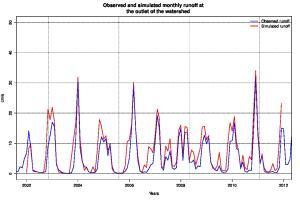
2002. 2004. 2006. 2008. 2010. 2012. 0. 10. 20. 30. 40. 50. Years cm/s. Observed and simulated monthly runoff at the outlet of the watershed. Observed runoff.

R Graphics Output -
Page 1. 100. 150. 200. 250. 300. 350. −15. −10. −5. 0. 5. 10 inla.group(agb, n = 100). PostMean 0.025% 0.5% 0.975%

R Graphics Output -
Page 1. q q q q q q q q q q q q. −9. −7. −5. −3. −1. 1. 3. 5. 01/17. 04/17. 07/17. 10/17. 01/18. Short−term changes (%) q q. Gross. Corrected.

R Graphics Output -
Page 1. q. 0.50. 0.75. 1.00. 1.25. 1.50. 0.50. 0.75. 1.00. 1.25. 1.50. 1. 1 test.

R Graphics Output -
0. 1. 2. 3. 4. 0. 100. 200. 300. 400. N55F 2017−05−04. Small−Scale. Time−lag (minutes). Semi−variance (square meters) q q q q q q. q q q q. q q q. q q q.

R Graphics Output -
2008 2009 2010 2011 2012 2013 2014 2015 2016. Clear Channel. PBSC/BIXI. BCycle. SandVault. Arcade. SOBI. Nextbike. Bewegen. Year. Number of systems ...

R Graphics Output -
Page 1. long lat. 60. 62. 64. 66. 68. 70. −60. −50. −40. −30. −20.