Recognizing RGB Images by Learning from RGB-D Data - IEEE Xplore

Viewer
Transcript

2014 IEEE Conference on Computer Vision and Pattern Recognition

Recognizing RGB Images by Learning from RGB-D Data Lin Chen1 Wen Li2 Dong Xu2 1 Institute for Infocomm Research, Agency for Science, Technology and Research, Singapore 2 School of Computer Engineering, Nanyang Technological University, Singapore Abstract

from the same data distribution. If one dataset is used for training and another dataset is used for testing, the performances of most existing visual recognition methods will degrade signiﬁcantly [28] because the feature distributions of samples from different datasets may have very different statistical properties. Meanwhile, to cope with the considerable variation in feature distributions, new domain adaptation methods were recently developed for different computer vision applications [15, 22, 14, 16, 7, 6, 10, 8, 13, 1].

In this work, we propose a new framework for recognizing RGB images captured by the conventional cameras by leveraging a set of labeled RGB-D data, in which the depth features can be additionally extracted from the depth images. We formulate this task as a new unsupervised domain adaptation (UDA) problem, in which we aim to take advantage of the additional depth features in the source domain and also cope with the data distribution mismatch between the source and target domains. To effectively utilize the additional depth features, we seek two optimal projection matrices to map the samples from both domains into a common space by preserving as much as possible the correlations between the visual features and depth features. To effectively employ the training samples from the source domain for learning the target classiﬁer, we reduce the data distribution mismatch by minimizing the Maximum Mean Discrepancy (MMD) criterion, which compares the data distributions for each type of feature in the common space. Based on the above two motivations, we propose a new SVM based objective function to simultaneously learn the two projection matrices and the optimal target classiﬁer in order to well separate the source samples from different classes when using each type of feature in the common space. An efﬁcient alternating optimization algorithm is developed to solve our new objective function. Comprehensive experiments for object recognition and gender recognition demonstrate the effectiveness of our proposed approach for recognizing RGB images by learning from RGB-D data.

In this work, we propose a new framework for recognizing RGB images captured with the conventional cameras by leveraging a set of labeled RGB-D data, in which the depth features can be additionally extracted from the depth images. Our work is based on the observation that several labeled RGB-D datasets were recently released for various vision recognition tasks [23, 21] as well as the recent progress on learning using privileged information [29, 26], which shows the additional features (i.e., privileged information) that are not available at the testing stage are still useful for many classiﬁcation tasks. We formulate our task as a new unsupervised domain adaptation (UDA) problem, in which we have the single-view visual features extracted from the RGB images in the target domain while we have both the visual features and the depth features in the source domain. Speciﬁcally, to effectively utilize the additional depth features in the source domain, we seek two optimal projection matrices to map the samples from both domains into a common space such that we can preserve as much as possible the correlations between the visual features and depth features. To effectively employ the source samples for learning the target classiﬁer, we reduce the data distribution mismatch between two domains by minimizing the Maximum Mean Discrepancy (MMD) criterion [17] for each type of feature in the common space, which compares the data distributions based on the distance between the means of samples from two domains. Motivated by the above two aspects, we propose a new SVM based objective function to simultaneously learn the two projection matrices and the optimal target classiﬁer, in which we expect the source samples from different classes can be well separated when using each type of feature in the common

1. Introduction With the rapid adoption of affordable equipments (e.g., Kinect sensors) for capturing depth information, there is an increasing research interest in developing new technologies for various visual recognition tasks (e.g., object recognition, face and gender recognition) using depth images. One common assumption in most visual recognition methods including the recent works using both color and depth images [23, 21] is that the training and testing samples come 1063-6919/14 $31.00 © 2014 IEEE DOI 10.1109/CVPR.2014.184

1412 1418

space. We also develop an efﬁcient alternating optimization algorithm to solve this non-trivial optimization problem. Our comprehensive experiments for object recognition and gender recognition demonstrate that our approach (referred to as domain adaptation from multi-view to singleview or DA-M2S in short) outperforms several state-of-theart methods including the existing UDA methods as well as SVM+ [29] and Rank Transfer [26] that use the depth features as privileged information without coping with the data distribution mismatch. We summarize the main contributions of this paper as follows: 1) we propose a new framework for recognizing RGB images by leveraging a set of labeled RGB-D data. From our framework, we formulate a new domain adaptation problem, where we have the additional features in the source domain that are not available in the target domain; 2) We propose a new UDA method DA-M2S and the extensive experiments demonstrate its effectiveness for recognizing RGB images by learning from RGB-D data.

2. Related Work

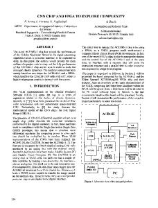
Figure 1. Object recognition in RGB images by using labeled RGB-D data, where we have two views of features (i.e., visual features and depth features) in the source domain, and a single view of visual features in the target domain. Grey color and black color respectively denote the projected nonlinear visual and depth features in the common space. The source domain samples from different categories are represented by different shapes and the unlabeled samples from the target domain are with question marks.

Domain Adaptation: Our work is related to domain adaptation, in which the distribution of test data is different from that of training data [20, 16, 15, 14, 13, 1, 7]. The existing unsupervised domain adaptation (UDA) methods assume there are no labeled data in the target domain and these methods can be generally divided into three categories: sample reweighting approaches, feature (transform) based approaches and classiﬁer based approaches. The sample reweighting approaches like kernel mean matching (KMM) [20] aim to reduce the domain distribution mismatch by reweighting the samples in the source domain. The feature (transform) based approaches seek new domain-invariant features or learn new feature transformations for domain adaptation. For example, SGF [16] and GFK [15] were proposed based on the Grassmann manifold assumption, and GFK was further extended in [14] by selecting the landmarks from the source domain. Recently, the domain invariant projection (DIP) [1] method was proposed to learn a domain invariant subspace, while the subspace alignment (SA) method [13] was developed to align two subspaces from two domains to reduce the domain distribution mismatch. The classiﬁer based approaches directly learn the target classiﬁers (e.g., SVM based classiﬁers) for domain adaptation. For example, Duan et al. [7] proposed a learning method called DAM by using the virtual labels generated from pre-learnt classiﬁers. However, the existing UDA methods assume the samples from the source domain share the same feature representation with those from the target domain. For these methods, it is unclear how to effectively utilize the additional depth features in the source domain. Recently, heterogeneous domain adaptation (HDA)

methods [9, 24, 22] were also proposed, in which the samples from different domains are generally represented by different types of features. However, labeled samples in the target domain must be provided in the existing HDA methods [9, 24, 22], while we do not require any labeled target domain samples in this work. Moreover, the samples in the source domain are represented by using only one type of features in the existing UDA and HDA methods. In contrast, in this work we have both visual and depth features in the source domain, while the depth features are not available at the testing stage. Our work is also different from the existing multiview domain adaptation methods [31] and the recent work called multi-domain adaptation from heterogeneous sources (MDA-HS) [3]. In [31], all the samples in the source and target domains have multiple types of features, while in [3] the samples from the target domain have all types of features from all the source domains. In contrast, in our work we only have single-view features in the target domain. Our work is different from existing multi-domain adaptation methods [7, 4], because we have additional depth features in the source domain. Learning Using Privileged Information: Our work is also related to the recent progress on learning using privileged information [29, 26], in which training data contains additional features (i.e., privileged information) that are not available at the testing stage. However, these works [29, 26] assume that the training and testing samples come from the same data distribution. In contrast, our work explicitly copes with the data distribution mismatch between two domains.

1419 1413

3. The Proposed Approach In this paper, we denote a vector/matrix by a lowercase/uppercase letter in bold. The transpose of a vector or a matrix is denoted by the superscript . We deﬁne In as the n × n identity matrix and On×m as the n × m matrix of all zeros. We also deﬁne 0n , 1n ∈ Rn as the n × 1 column vectors of all zeros and all ones, respectively. For simplicity, we use I, O, 0 and 1 when the dimension is obvious.

3.1. Problem Setup In our problem, given a set of labeled RGB-D data in the source domain and unlabeled RGB images in the target domain, we aim to learn a robust classiﬁer to predict the class labels of RGB images in the target domain. We extract visual features and depth features from the RGB images and depth images, respectively. The source s } domain samples can be represented as {(zi , xsi , yi )|ni=1 s where zi and xi are respectively the depth feature and the visual feature and yi ∈ Y is the label for the i-th source domain sample with Y = {1, . . . , K} being the set of all possible labels and ns is the total number of samples in the source domain. We also denote y = [y1 , ..., yns ] as the label vector for the source domain samples. Similarly, the tart } where get domain samples can be represented as {xti |ni=1 t xi is the visual feature for the i-th target domain sample and nt is the total number of samples in the target domain. As shown in Fig. 1, the major challenges are from different features and the data distribution mismatch between two domains. To handle the ﬁrst challenge, we propose to project different features into a common space by learning two projection matrices Pd and Pv for the depth features (i.e., z) and visual features (i.e., xs and xt ), respectively. The two types of features are transformed to the same representation in this common space by using the learnt projection matrices. Moreover, to handle the data distribution mismatch between two domains, we also minimize the Maximum Mean Discrepancy (MMD) [17] criterion for each type of feature in the common space. Then we can learn a robust classiﬁer which aims to well separate all the source domain labeled samples in this common space. Intuitively, a suitable common space will be beneﬁcial for learning a more robust classiﬁer; and the robust classiﬁer can also help us ﬁnd a more discriminative common space. Therefore, we propose to simultaneously seek the projection matrices and learn the optimal classiﬁer. Based on the empirical risk minimization (ERM) principle, we formulate our learning problem as follows: min

f,Pv ,Pd

μΩ(Pd , Pv ) + r(f ) + C(f, Pd , Pv ),

(1)

where f is the target classiﬁer, r(f ) is the regularizer term to control the complexity of the classiﬁer, Ω(·) is the regularizer term on the projection matrices Pv and Pd , (·) is

the loss on the training samples, and μ and C are the tradeoff parameters. We will introduce the details of these terms below.

3.2. The Formulation For the sake of generality, we consider the kernelized case in this work, i.e., the projection matrices Pd and Pv are learnt based on the nonlinear features induced by the kernels of the depth features and visual features. The linear case can be easily derived in a similar manner. Formally, let us denote the nonlinear depth feature as ψ(z) ∈ Rmd and the nonlinear visual feature as φ(x) ∈ Rmv where md and mv are respectively the dimensions of the nonlinear depth feature and the nonlinear visual feature, which are usually unknown. Then the projection matrices can be deﬁned as Pd ∈ Rmd ×m and Pv ∈ Rmv ×m , respectively, where m is the dimension of the common space. Intuitively, we should preserve as much as possible the useful information from the original features when learning the projection matrices Pd and Pv . Inspired by the multiview learning method KCCA [19], we propose to maximize the correlation between the two types of features based on correspondence information between the two views of features in the source domain. Namely, we minimize the following regularizer: Ωkcca (Pd , Pv ) = −tr(Pd ΨΦs Pv ),

(2)

where Ψ = [ψ(z1 ), . . . , ψ(zns )] ∈ Rmd ×ns and Φs = [φ(xs1 ), . . . , φ(xsns )] ∈ Rmv ×ns are the data matrices of the nonlinear depth and visual features in the source domain. To avoid the trivial solutions for Pd and Pv , we also introduce the constraint Pd ΨΨ Pd + Pv Φs Φs Pv = Im . Moreover, to handle the distribution mismatch between the source and target domains, we also expect the distributions of samples from different domains are similar in the common space. Speciﬁcally, we employ the Maximum Mean Discrepancy (MMD) [17] criterion to measure the distribution mismatch between two domains. Considering we have two types of features in the source domain, we apply the MMD criterion for each type of feature in the common space, and obtain the following regularizer: 2 ns nt 1 1 1 s t mmd (Pd , Pv )= Pv φ(xi ) − Pv φ(xj ) Ω 2 ns i=1 nt j=1 2 ns nt 1 1 1 t + Pd ψ(zi ) − Pv φ(xj ) . 2 ns i=1 nt j=1 Then, our regularizer Ω(Pd , Pv ) in (1) can be obtained by combining the two regularizers: Ω(Pd , Pv ) = Ωkcca (Pd , Pv ) + λΩmmd (Pd , Pv ),

1420 1414

(3)

where λ is a tradeoff parameter for balancing the two terms. Now we develop the detailed form of our DA-M2S method1 based on multi-class SVM [5]. For ease of presentation, we denote one training sample in the common ˜ , which can be Pd ψ(z) or Pv φ(xs ). So in total space as x we have 2ns labeled samples in the source domain, where ns samples are based on the visual features and the other ns samples are based on the depth features. We deﬁne the ˜ with wk decision function as f (˜ x) = argmaxk=1,...,K wk x being the weight vector for the k-th class. By deﬁning a matrix W = [w1 , . . . , wK ], we write the objective function in (1) as follows: n 1 μΩ(Pd , Pv ) + W2F + C ξi , (4) min 2 (Pd ,Pv )∈P, i=1 W,ξi

s.t.

˜ i − wk x ˜ i ≥ eki − ξi , wy i x ∀i = 1, . . . , 2ns , k = 1, . . . , K,

(5)

where W2F is the regularizer to control the complexity of the classiﬁer f , eki is an indicator which equals to 0 if yi = k and 1 otherwise, P = {(Pd , Pv )|Pd ΨΨ Pd + Pv Φs Φs Pv = Im } is the feasible set of (Pd , Pv ), and μ and C are the tradeoff parameters as deﬁned in (1).

3.3. The Duality Since the dimensions of the nonlinear features ψ(z) and φ(x) (i.e., md and mv ) are usually unknown, in this section, we derive the kernel form of the problem in (4) using the Lagrangian method. First, similar as in KCCA, we represent the projection matrices as the combination of the nonlinear features, i.e., Pd = ΨAd , Pv = Φs Av where Ad , Av ∈ Rns ×m are the combination coefﬁcient matrices. We also deﬁne a matrix A = [Ad , Av ] ∈ R2ns ×m , and then the regularizer in (2) becomes, 1 Ωkcca (A) = − tr(A Bkcca A), (6) 2 where O Kd Ksv kcca , = B Ksv Kd O with Kd = Ψ Ψ ∈ Rns ×ns being the kernel matrix for the source domain depth features, and Ksv = Φs Φs ∈ Rns ×ns being the kernel matrix for the source domain visual features. Similarly, the regularizer Ωmmd (Pd , Pv ) can be represented as 1 Ωmmd (A) = tr(A Bmmd A), (7) 2 where O O Kd mmd Kd B , ss = Ksv 2Kst Ksv 2Kst v v 1 Note

lations.

our method can be readily extended to other SVM based formu-

ns ×nt being the kernel matrix bewith Kst v = Φs Φ t ∈ R tween the source data and target data based on the visual features, Φt = [φ(xt1 ), . . . , φ(xtnt )] ∈ Rmv ×nt being the data matrix of nonlinear visual features in the target domain, and s = [ n1s 1ns , − n1t 1nt ] ∈ R(ns +nt ) . Let us deﬁne B = Bkcca − λBmmd ∈ R2ns ×2ns . Combining (6) and (7), we represent our regularizer Ω(Pv , Pd ) in (3) w.r.t. A as follows: 1 Ω(A) = − tr(A BA). 2

Moreover, the feasible set P in (4) becomes A = {A = [Ad , Av ] |Ad Kd Kd Ad + Av Ksv Ksv Av = Im }. By introducing one dual variable αik for each constraint in (5) and deﬁning a matrix Γ ∈ R2ns ×K with its (i, k)-th entry as γik = 1 − eki − αik , we write the dual form of (4) as follows: (8) min μΩ(A) + max J(A, Γ) , A∈A

Γ∈M

where J(A, Γ) = − 12 tr(Γ KA Γ) − tr(E Γ), and E ∈ R2ns ×K is a matrix with its (i, k)-th entry as eki , M = {Γ|Γ1K = 02ns , γik ≤ C(1 − eki )} is the feasible set of Γ, and KA ∈ R2ns ×2ns is the kernel matrix for the samples in the common space, which is deﬁned as follows: Kd O O Kd AA . KA = O Ksv O Ksv Note that the similarities between the depth features and visual features are also integrated in KA by associating with the combination coefﬁcient matrix A.

4. Solution The problem in (8) is a non-convex problem w.r.t A and Γ. Therefore, we propose an alternating optimization algorithm to solve it, in which we use line search when solving for A at each iteration to ensure the decrease of the objective in (8). Speciﬁcally, given the combination coefﬁcient matrix A, the optimization problem in (8) becomes max

Γ∈M

1 − tr(Γ KA Γ) − tr(E Γ), 2

(9)

which is a multi-class SVM problem, and can be solved efﬁciently by using the existing solver2 in LIBLINEAR [11]. On the other hand, when we ﬁx Γ, the optimization problem w.r.t. A can be written as 1 ˜ min − tr(A BA), (10) A∈A 2 2 Note

A

1421 1415

Kd O

KA can be treated as a linear kernel with the data matrix as O ∈ Rm×2ns . Ksv

Kd O Γ ∈ O Ksv R2ns ×K . It shares the similar formulation with KCCA which can be solved by using the generalized eigendecomposition. It is worth mentioning that the matrix B in our problem integrates the unlabeled samples from the target domain [see (7)], and the matrix G also integrates the dual variables of the classiﬁer f in Γ, which indicate that the target domain unlabeled samples and the classiﬁer learnt at the previous iteration also contribute to the learning of the common space in (10). ˜ = μB + GG with G = where B

4.1. Line Search when Solving for A Due to the non-convexity of (8), the optimal solution A∗ from (10) cannot ensure the objective of (8) decreases. Therefore, at the t-th iteration, we need to search for a feasible At ∈ A between the optimal solution A∗ and the solution At−1 at the previous iteration. In the following, we ﬁrst brieﬂy introduce how to solve for the optimal solution A∗ to the problem in (10), then we present our line search method. 4.1.1 Solving for A∗ The problem in (10) can be reformulated as a generalized eigen-decomposition problem [19] as follows: ˜ = σDv, Bv (11) O Kd Kd ∈ R2ns ×2ns , v is the eigenwhere D = O Ksv Ksv vector and σ is the corresponding eigenvalue. The optimal solution to (10) is obtained by combining the m leading eigenvectors corresponding to the largest eigenvalues. To solve (11), we ﬁrst perform the incomplete Cholesky decomposition on D as D = C C as suggested in [19]. Then, we can rewrite (11) as a standard eigen˜ −1 u = σu, where u = decomposition problem, (C−1 ) BC −1 ˜ −1 Cv is the eigenvector of (C ) BC . ˜ −1 Let us denote the eigen-decomposition of (C−1 ) BC as UΣU where U is the eigenvectors and Σ is a diagonal matrix with the diagonal entries being the eigenvalues. ˜ ∗ ∈ R2ns ×m as the matrix containing the We also deﬁne U m leading eigenvectors in U corresponding to the largest eigenvalues. Then, the optimal solution to (10) can be ob˜ ∗. tained as A∗ = C−1 U 4.1.2

Line Search for At

The major challenge in line search is to ensure that the solution satisﬁes the constraint At ∈ A. Note that the feasible ˜ where U ˜ ∈ R2ns ×m A is given in the form of A = C−1 U ˜ is an orthogonal matrix. Let S = span(U) be the subspace ˜ Obviously, all basis matrices of the subspace spanned by U. S are feasible, and produce equal objective value in (8).

Algorithm 1 The algorithm for our DA-M2S Input: The label vector y, and the kernel matrices Kd , Ksv and Kst v as deﬁned in Section 3.3. 1: Initialize t = 0. 2: Solve (8) with only the ﬁrst term [i.e., Ω(A)] to obtain ˜ 0. an initial A0 = C−1 U 3: Solve for Γ0 in (9) based on A0 by using the existing solver in LIBLINEAR [11]. 4: repeat 5: Set t = t + 1. ˜ ∗. 6: Solve the problem in (11) to obtain A∗ = C−1 U ˜ 7: Find the optimal basis U(τ ) in the geodesic path such that the objective in (8) is minimized. ˜ ) by using the 8: Solve Γ based on A(τ ) = C−1 U(τ existing solver in LIBLINEAR [11]. 9: Set At = A(τ ), Γt = Γ. 10: until The objective in (8) converges. Output: A = At and Γ = Γt . ˜ t−1 as the solution to Let us denote At−1 = C−1 U ˜ ∗ as the (10) at the previous iteration, and A∗ = C−1 U optimal solution at this iteration, respectively. Recall that all 2ns -by-m subspaces reside on a Grassmann manifold, so our line search problem becomes to ﬁnd a new subspace St along the geodesic path between two subspaces ˜ t−1 ) and S ∗ = span(U ˜ ∗ ), whose basis St−1 = span(U ˜ Ut makes the objective of (8) decrease. As shown in [16], the geodesic path between St−1 and S ∗ can be represented as S(τ ) with 0 ≤ τ ≤ 1, and we have S(0) = St−1 and S(1) = S ∗ . Then, we perform line search using different τ ’s to ﬁnd a subspace S(τ ) = ˜ )) according to the method in [16] such that the span(U(τ ˜ ) leads to the minimal projection matrix A(τ ) = C−1 U(τ objective in (8). Finally, the details of our algorithm for solving (8) are listed in Algorithm 1. We ﬁrst initialize the combination coefﬁcient matrix A by solving (8) with only the ﬁrst term [i.e., Ω(A)]. Then, we iteratively solve (9) by using the existing solver in [11] and solve the eigenvalue decomposition problem in (11). Then we perform the line search between St−1 and S ∗ to ﬁnd a better subspace St , such ˜ t leads to the minimal objective in (8). that At = C−1 U The above procedure is repeated until the objective value no longer decreases. In our experiments, the algorithm converges after about 10 iterations. By using the learnt A = [Ad , Av ] , any test data xt from the target domain can be projected into the common space ˜ t = Pv φ(xt ) = Av Φs φ(xt ). Then we can use the as x learnt classiﬁer to predict its class label. The ﬁnal classiﬁer ˜ t , where each is given by f (˜ xt ) = argmaxk=1,...,K wk x 2ns k k ˜ i , in which γi is the (i, k)-th entry of Γ wk = i=1 γi x ˜ i is the i-th training sample from from Algorithm 1, and x the source domain in the common space.

1422 1416

5. Experiments

only color images. In this work, we use the 10 common categories3 between the two datasets. As the RGB-D Object dataset is recorded in the form of video sequences, we uniformly sample the frames with an interval of two seconds, leading to a total number of 2059 training images. All the target domain samples are also used as unlabeled data in the training stage for the baseline domain adaptation methods and our DA-M2S. We use kernel descriptors (KDES) features [2] in this work, which have shown promising recognition results on this dataset. Speciﬁcally, we extract Gradient KDES and LBP KDES features from each RGB/depth image by using the software4 provided by the authors. Then, we follow [2] to aggregate the kernel descriptors into object-level features, in which we set the vocabulary size as 1000 and use three level of pyramids (i.e., 1x1, 2x2, 3x3). The object level features respectively constructed from the Gradient KDES and LBP KDES features are concatenated into one feature vector for each RGB/depth image. Note the features for RGB and depth images are different, because we use different vocabularies. We use the same method to extract the visual features for the RGB images in the target domain. We use the multiclass classiﬁcation accuracy as the evaluation criterion, which is the average of the accuracies over all the classes. For all the kernel-based approaches, Gaussian kernel is used as the default kernel with the bandwidth parameter set as the mean of the distances between any two samples. We use the default tradeoff parameter C = 1 for all methods. Moreover, for our DA-M2S, we empirically ﬁx the parameters as μ = 0.1ns and λ = 104 . For all other methods, we tune their parameters based on the test dataset and report their best results from the optimal parameters. Experimental Results: The results of all methods are reported in Table 1. From this table, we observe that our newly proposed DA-M2S outperforms all other baseline methods. It demonstrates the effectiveness of our DA-M2S by employing the additional depth features in the source domain and simultaneously reducing the domain distribution mismatch between the source and target domains. Speciﬁcally, by utilizing the additional depth features, the multi-view learning approaches KCCA and SVM2K as well as the privileged learning approach SVM+ achieve better results when compared with the naive approach SVM A. RT is worse than SVM A, possibly because it is based on RankSVM, which is designed for the ranking task rather than the classiﬁcation task. Among these methods, SVM2K achieves the best result, as it can more effectively exploit depth information by learning two classiﬁers for both vi-

In this section, we evaluate the effectiveness of our DA-M2S for object recognition and gender recognition.

5.1. Baseline Approaches To the best of our knowledge, there is no previous work speciﬁcally designed for recognizing RGB images by learning from RGB-D data. Thus, we extend a broad range of existing works as the baselines for fair comparison, which can be divided into four categories as follows: Naive Approach: The naive approach SVM A is trained by using the visual features in the source domain without considering the domain distribution mismatch and exploiting the additional depth features. Multi-view Learning: The multi-view learning approaches include KCCA [19] and SVM2K [12], in which the twoview data in the source domain are used for training. For SVM2K, two classiﬁers are trained by using the two-view data in the source domain, and we use the one based on visual features to predict the target domain visual features. For KCCA, we train two SVM classiﬁers by using the projected depth and visual features in the common space and the decision values of target domain samples based on the projected visual features are equally fused for prediction. Learning Using Privileged Information: For the learning approaches using privileged information such as SVM+ [29] and RankTransfer (RT) [26], we use the additional depth features in the source domain as privileged information for learning the visual feature based classiﬁer. Unsupervised Domain Adaptation: The domain adaptation approaches include KMM [20], DAM [7], SGF [16], TCA [25], Landmark (LMK) [14], Subspace Alignment (SA) [13], and Domain Invariant Projection (DIP) [1], for which the visual features from both domains are used for training the classiﬁers and we predict target domain data based on the visual features. We do not compare our DA-M2S with GFK [15], because the subsequent work LMK from the same group is shown to be better (see [14]). Note that the semi-supervised multi-view learning methods [27] and the multi-view domain adaptation approaches [31] cannot be applied for our problem, because we only have single view of features for the samples in the target domain. Moreover, the heterogeneous domain adaptation (HDA) methods [22, 24] also cannot be used because the labeled samples in the target domain are required in these HDA methods.

5.2. Object Recognition Experimental Setup: We evaluate our proposed DA-M2S for object recognition by using the RGB-D Object dataset [23] as the source domain and the Caltech-256 dataset [18] as the target domain. The RGB-D Object dataset contains the color and depth images of different objects from 51 categories. The Catech-256 dataset contains

3 The 10 common categories between the two datasets are calculator, cereal box, coffee mug, keyboard, ﬂashlight, lightbulb, mushroom, ball, soda can, tomato. 4 The code is available at http://www.cs.washington.edu/ai/Mobile Robo tics/projects/kdes/.

1423 1417

Table 1. Comparison of recognition accuracies (%) for object recognition. The RGB-D object dataset is used as the source domain and the Caltech-256 dataset is used as the target domain.

SVM A SVM+ RT KCCA SVM2K KMM DAM SGF LMK TCA SA DIP DA-M2S 18.19 18.59 17.16 18.23 20.83 18.10 18.19 19.25 19.45 25.07 21.09 25.47 30.06 Table 2. Recognition accuracies (%) of domain adaptation methods for object recognition using the feature representations in the common space learnt by KCCA.

ment. All face images in two datasets are aligned and cropped to a ﬁxed size of 120 × 105 pixels according to the positions of two eyes. The images in the LFW-a dataset have been aligned according to the eye-positions (see [30] for details). For the EURECOM dataset, the manually annotated eyepositions are provided, and the images with only a single eye-position (i.e. the proﬁle face images) are not included in our experiments as suggested in [21]. Then, we uniformly divide each face image into 8 × 7 non-overlapping subregions with the size of each subregion being 15 × 15 pixels. After that, we extract the Gradient-LBP feature [21] from each subregion for both color and depth images, as it has been shown to be effective for gender recognition [21]. Finally, for each face image, the Gradient-LBP features from all 56 subregions are concatenated into a single feature vector. The same Gradient-LBP features are also extracted for the RGB images in the LFW-a dataset.

KMM-C DAM-C SGF-C LMK-C TCA-C SA-C DIP-C 18.47 17.50 19.38 19.72 27.48 21.25 24.76 sual and depth features. Nevertheless, all these methods do not cope with the distribution mismatch between the source and target domains, thus they are much worse than our DA-M2S. The domain adaptation methods SGF, LMK, TCA, SA and DIP are also better than SVM A, which shows it is beneﬁcial to reduce the domain distribution mismatch between the source and target domains by using these methods. When compared with SVM A, KMM and DAM are only comparable or even worse, possibly because both approaches cannot effectively handle the signiﬁcant domain distribution mismatch in this application. Moreover, our proposed DA-M2S outperforms all those methods by additionally exploiting the depth features in the source domain. KCCA + UDA Approaches: We additionally report more results for object recognition by using the domain adaptation methods in the common space learnt by using KCCA, which are referred to as KMM-C, DAM-C, SGF-C, LMKC, TCA-C, SA-C and DIP-C. Speciﬁcally, we ﬁrst learn the projection matrices by using KCCA and project both visual and depth features into the learnt common space. Then, we apply these domain adaptation methods using the projected depth and visual features in the common space to learn two classiﬁers and equally fuse the decision values of target samples from two classiﬁers using the projected visual features. The results are shown in Table 2. We observe that most UDA methods are improved by utilizing the additional depth features, when compared with their corresponding results in Table 1. Our DA-M2S still outperforms those baselines, which again demonstrates it is beneﬁcial to simultaneously employ the additional depth features and reduce the domain distribution mismatch.

Because there are much more male faces than female faces in the EURECOM dataset, we randomly sample 196 male faces from this dataset to balance the positive and negative training samples. We also randomly sample 3,000 samples from a large number of target samples as unlabeled data for the baseline domain adaptation methods and our DA-M2S. The mean recognition accuracy and the standard deviation over ten rounds of experiments are reported for all the methods for gender recognition. The rest of the settings are the same as in object recognition. Experimental Results: The results of SVM+ and RT are 64.24 ± 1.66 and 64.22 ± 1.76 respectively, and the results of all other methods are shown in Table 3. We have similar observations as in the object recognition. While other methods generally outperform SVM A by exploiting the additional depth features or reducing the domain distribution mismatch, our DA-M2S outperforms all the baseline methods by simultaneously considering both aspects in one formulation.

5.3. Gender Recognition Experimental Setup: We also evaluate our DA-M2S for gender recognition by using the RGB-D face dataset EURECOM [21] as the source domain, and the RGB dataset Labeled Faces in the Wild-a (LFW-a) [30] as the target domain. The EURECOM dataset [21] contains the RGB and depth images captured by using the Kinect sensor. There are totally 728 pairs of RGB and depth images from 196 females and 532 males. The LFW-a dataset contains a total number of 13, 144 images from 2, 960 females and 10, 184 males, which are collected under the uncontrolled environ-

We also observe that SVM2K is much better than SVM A, demonstrating that it is beneﬁcial to use the additional depth features in the source domain for this application. However, KCCA, SVM+ and RT are not as effective as SVM2K, and they are only comparable to or even worse than SVM A. Most of the domain adaptation approaches such as SGF, LMK, TCA, SA and DIP are also better than SVM A. However, KMM and DAM are only comparable or even worse than SVM A in this application.

1424 1418

Table 3. Comparison of recognition accuracies (mean ± standard deviation %) for gender recognition. The result in bold is signiﬁcantly better than the others judged by the signiﬁcant test with a signiﬁcance level of 0.05. SVM A KCCA SVM2K KMM DAM SGF LMK TCA SA DIP DA-M2S 64.22±1.6 63.60±1.34 67.33±1.92 64.25±1.43 63.91±1.57 67.22±1.38 65.02±1.55 65.24±0.88 67.38±1.39 64.84±4.80 68.44±1.44 Table 4. Comparison of recognition accuracies (%) between DA-M2S and its special cases.

DA-M2S (w/o depth) DA-M2S (init) DA-M2S

Gender 67.57±1.68 67.39±1.02 68.44±1.44

[3] L. Chen, L. Duan, and D. Xu. Event recognition in videos by learning from heterogeneous web sources. In CVPR, pages 2666–2673, 2013. [4] K. Crammer, M. Kearns, and J. Wortman. Learning from multiple sources. JMLR, 9:1757–1774, 2008. [5] K. Crammer and Y. Singer. On the algorithmic implementation of multiclass kernel-based vector machines. JMLR, 2:265–292, 2002. [6] L. Duan, I. W. Tsang, and D. Xu. Domain transfer multiple kernel learning. T-PAMI, 34(3):465–479, March 2012. [7] L. Duan, I. W. Tsang, D. Xu, and T. Chua. Domain adaptation from multiple sources: A domain-dependent regularization approach. T-NNLS, 23(3):504– 518, 2012. [8] L. Duan, D. Xu, and S.-F. Chang. Exploiting web images for event recognition in consumer videos: A multiple source domain adaptation approach. In CVPR, pages 1338–1345, 2012. [9] L. Duan, D. Xu, and I. W. Tsang. Learning with augmented features for heterogeneous domain adaptation. In ICML, pages 711–718, 2012. [10] L. Duan, D. Xu, I. W. Tsang, and J. Luo. Visual event recognition in videos by learning from web data. T-PAMI, 34(9):1667–1680, September 2012. [11] R. Fan, K. Chang, and C. Hsieh. LIBLINEAR: A library for large linear classiﬁcation. JMLR, 9:1871–1874, 2008. [12] J. D. R. Farquhar, H. Meng, S. Szedmak, D. R. Hardoon, and J. Shawe-taylor. Two view learning: SVM-2K, theory and practice. In NIPS, 2006. [13] B. Fernando, A. Habrard, M. Sebban, and T. Tuytelaars. Unsupervised visual domain adaptation using subspace alignment. In ICCV, 2013. [14] B. Gong, K. Grauman, and F. Sha. Connecting the dots with landmarks: Discriminatively learning domain-invariant features for unsupervised domain adaptation. In ICML, 2013. [15] B. Gong, Y. Shi, F. Sha, and K. Grauman. Geodesic ﬂow kernel for unsupervised domain adaptation. In CVPR, 2012. [16] R. Gopalan, R. Li, and R. Chellappa. Domain adaptation for object recognition: An unsupervised approach. In ICCV, 2011. [17] A. Gretton, K. M. Borgwardt, M. J. Rasch, B. Sch¨olkopf, and A. Smola. A kernel two-sample test. JMLR, 13:723–773, 2012. [18] G. Grifﬁn, A. Holub, and P. Perona. Caltech-256 object category dataset. Technical report, California Institute of Technology, 2007. [19] D. R. Hardoon, S. R. Szedmak, and J. R. Shawe-taylor. Canonical correlation analysis: An overview with application to learning methods. Neural Computing, 16(12):2639–2664, 2004. [20] J. Huang, A. Smola, A. Gretton, K. Borgwardt, and B. Scholkopf. Correcting sample selection bias by unlabeled data. In NIPS, 2007. [21] T. Huynh, R. Min, and J.-L. Dugelay. An efﬁcient LBP-based descriptor for facial depth images applied to gender recognition using RGB-D face data. In ACCV Workshop, 2012. [22] B. Kulis, K. Saenko, and T. Darrell. What you saw is not what you get: Domain adaptation using asymmetric kernel transforms. In CVPR, 2011. [23] K. Lai, L. Bo, X. Ren, and D. Fox. A large-scale hierarchical multi-view RGB-D object dataset. ICRA, 2011. [24] W. Li, L. Duan, D. Xu, and I. W. Tsang. Learning with augmented features for supervised and semi-supervised heterogeneous domain adaptation. T-PAMI, 2013. [25] S. J. Pan, I. W. Tsang, J. T. Kwok, and Q. Yang. Domain adaptation via transfer component analysis. T-NN, 22(2):199–210, 2009. [26] V. Sharmanska, I. Austria, N. Quadrianto, and C. Lampert. Learning to rank using privileged information. In ICCV, 2013. [27] V. Sindhwani, P. Niyogi, and M. Belkin. A coregularization approach to semisupervised learning with multiple views. In ICML, 2005. [28] A. Torralba and A. A. Efros. Unbiased look at dataset bias. In CVPR, 2011. [29] V. Vapnik and A. Vashist. A new learning paradigm: learning using privileged information. Neural networks, 22(5-6):544–57, 2009. [30] L. Wolf, T. Hassner, and Y. Taigman. Effective unconstrained face recognition by combining multiple descriptors and learned background statistics. T-PAMI, 33(10):1978–1990, 2011. [31] D. Zhang, J. He, Y. Liu, L. Si, and R. D. Lawrence. Multi-view transfer learning with a large margin approach. In KDD, 2011.

Object 28.45 28.43 30.06

5.4. Analysis on DA-M2S For a better understanding of our DA-M2S, we investigate two special cases of our DA-M2S. In the ﬁrst special case, denoted as DA-M2S (w/o depth), we do not consider depth information. Namely, we remove Ωkcca (Pd , Pv ) as well as the second term of Ωmmd (Pd , Pv ) in the regularizer Ω(Pd , Pv ) in (4). Note Ω(Pd , Pv ) becomes Ω(Pv ) with Pv ∈ P, where P = {Pv |Pv Φs Φs Pv = Im }. We also remove the ns constraints related to the depth features in (5). As shown in Table 4, the results are worse than our DA-M2S, which shows it is beneﬁcial to exploit the additional depth features for learning a more robust classiﬁer. We also report the results of our DA-M2S at the ﬁrst iteration, which is denoted as DA-M2S (init). As show in Table 4, its performances are also worse than DA-M2S, which demonstrates the effectiveness of our alternating optimization technique for iteratively learning the classiﬁer and the projection matrices.

6. Conclusions In this paper, we have proposed a new framework for recognizing RGB images by learning from a set of labeled RGB-D data. We formulate this task as a new UDA problem, in which we have both visual and depth features in the source domain, while we only have the visual features in the target domain. An effective method called DA-M2S is proposed to solve this problem by taking advantage of the additional depth features in the source domain and simultaneously reducing the distribution mismatch between the source and target domains. Comprehensive experiments for object recognition and gender recognition have clearly demonstrated the effectiveness of our proposed DA-M2S approach for recognizing RGB images by learning from RGB-D data. Acknowledgement. This work is supported by the Singapore MoE Tier 2 Grant (ARC42/13).

References [1] M. Baktashmotlagh, M. Harandi, and M. S. Brian Lovell. Unsupervised domain adaptation by domain invariant projection. In ICCV, 2013. [2] L. Bo, X. Ren, and D. Fox. Depth kernel descriptors for object recognition. In IROS, 2011.

1425 1419