Scalable Spatial Scan Statistics through Sampling Michael Matheny Raghvendra Singh Liang Zhang Kaiqiang Wang Jeff M. Phillips School of Computing University of Utah
ACM SigSpatial, 2016
Spatial Scan Statistics Sampled Philadelphia crime data I
Theft
I
All crimes in red and blue
Spatial Scan Statistics I
Data set X ⊆ R2 and for each x ∈ X I I
I
Sets defined by regions A ⊂ 2X . I I
I
m(x) is a measured value. m(x) = 1 for theft otherwise 0. b(x) is a baseline value. b(x) = 1 for all points. Disks Rectangles
Find region that maximizes function φ.
Spatial Scan Statistics Want to find regions corresponding to: I
Disease outbreaks
I
High regions of crime
I
Environmental causes for cancer
I
Wildfires, earthquakes, and other natural disasters.
Anomaly Detection Pipeline
I
Formulate a model of the data and choose a corresponding measure φ to score the likelihood of an anomaly in a region.
Anomaly Detection Pipeline
I
Formulate a model of the data and choose a corresponding measure φ to score the likelihood of an anomaly in a region.
I
Scan the data set to find a region A which maximizes φ.
Anomaly Detection Pipeline
I
Formulate a model of the data and choose a corresponding measure φ to score the likelihood of an anomaly in a region.
I
Scan the data set to find a region A which maximizes φ.
I
Assess whether the score φ(A) indicates A is significant.
Anomaly Detection Pipeline
I
Formulate a model of the data and choose a corresponding measure φ to score the likelihood of an anomaly in a region.
I
Scan the data set to find a region A which maximizes φ.
I
Assess whether the score φ(A) indicates A is significant.
Existing Approaches For set |X | = m. I SatScan [Kul97] [Kul06] I I I
I
Commonly used. Scans all disks. O(m3 log(m)) runtime.
Agarwal [AMP+ 06] I I I
Approximation using linear functions. Faster and works on rectangles. O( ε1 m2 log2 (m)) runtime.
Existing Approaches For set |X | = m. I Neill [NM04] I I I I
Aggregates to grid. Can miss anomalies if dense clusters of points exist. Performance depends on data. Best Case O(g 2 log(g )), Worst Case O(g 4 ).
Data is usually a Sample
Methods assume entire data set is available, but... I
Only reported crimes.
I
Census samples population.
I
1% feed of geolocated tweets.
How much error does sampling introduce in anomaly detection?
Algorithms
Sample Then Scan Idea: Run SatScan on Sample.
Sample Then Scan Problem: Far too many combinatorial regions.
Sample Then Scan Idea: Use smaller sample to induce regions.
Sample Then Scan Idea: Use smaller sample to induce regions.
Sample Then Scan Compute φ using dense sample.
Sample Then Scan Compute φ using dense sample.
Sample Then Scan Compute φ using dense sample.
Enumerating Disks I
Split points along half space defined by points p1 , p2 ∈ N (sparse sample)
I
Sort S (dense sample) by the order points fall into a disk passing through p1 and p2 .
Enumerating Disks I
Split points along half space defined by points p1 , p2 ∈ N (sparse sample)
I
Sort S (dense sample) by the order points fall into a disk passing through p1 and p2 .
Enumerating Disks I
Split points along half space defined by points p1 , p2 ∈ N (sparse sample)
I
Sort S (dense sample) by the order points fall into a disk passing through p1 and p2 .
Enumerating Disks I
Split points along half space defined by points p1 , p2 ∈ N (sparse sample)
I
Sort S (dense sample) by the order points fall into a disk passing through p1 and p2 .
Enumerating Disks I
Split points along half space defined by points p1 , p2 ∈ N (sparse sample)
I
Sort S (dense sample) by the order points fall into a disk passing through p1 and p2 .
I
Repeat for all p1 and p2 .
I
|N| = n, |S| = s
I
O(n2 s log(n))
Enumerating Rectangles
I
Use N to define a grid of size n2
I
Distribute points in S into grid cells
I
Enumerate over all lower and upper corners.
I
O(n4 + s log(n))
Can this Work? If this works then we help scalability and the sampling problem. I
How well does this method work in practice?
I
Can we prove guarantees?
How well does this work?
Experimental Setup
I I
5 million tweets. Algorithm ran with: I I
I
Planted region containing: I I I
I
|N| = n sparse sample. |S| = s dense sample. r fraction of points. p measured rate outside. q measured rate inside.
Jaccard Distance d(A, B) = 1 −
|A ∩ B |A ∪ B|
Stability
Defaults I
Outside rate p = .04
I
Inside rate q = .08
I
Region size r = .05
I
Sparse sample n = 100
I
Large sample s = 4000
Stability
Defaults I
Outside rate p = .04
I
Inside rate q = .08
I
Region size r = .05
I
Sparse sample n = 100
I
Large sample s = 4000
Stability
Defaults I
Outside rate p = .04
I
Inside rate q = .08
I
Region size r = .05
I
Sparse sample n = 100
I
Large sample s = 4000
Stability
Defaults I
Outside rate p = .04
I
Inside rate q = .08
I
Region size r = .05
I
Sparse sample n = 100
I
Large sample s = 4000
Stability
Defaults I
Outside rate p = .04
I
Inside rate q = .08
I
Region size r = .05
I
Sparse sample n = 100
I
Large sample s = 4000
Stability
Defaults I
Outside rate p = .04
I
Inside rate q = .08
I
Region size r = .05
I
Sparse sample n = 100
I
Large sample s = 4000
Running Time Defaults I
Outside rate p = .04
I
Inside rate q = .08
I
Region size r = .05
I
Sparse sample n = 100
I
Large sample s = 4000
alldisks: O(n2 s log(n)) allrect: O(n4 + s log(n))
Running Time Method compares favorably with existing algorithms when using similar error.
Unlike griding our methods have guarantees since sample N adapts to data.
Experiment Summary
I
Reasonable sample sizes.
I
Finds region with high overlap.
I
Stable results till threshold.
I
Very fast.
Why does this work?
Lipschitz Bounds Need approximation on the Kulldorff Scan Statistic φX (A) = mA ln
If: I ερ ≥ |mA − m ˆA| 2 ερ ˆ I 2 ≥ |bA − bA | I ρ-boundary conditions.
Then |φ(mA , bA ) − φ(m ˆ A , bˆA )| ≤ ε.
1 − mA mA + (1 − mA ) ln . bA 1 − bA
Lipschitz Bounds Need approximation on the Kulldorff Scan Statistic φX (A) = mA ln
If: I ερ ≥ |mA − m ˆA| 2 ερ ˆ I ≥ |bA − bA | 2 I ρ-boundary conditions.
Then |φ(mA , bA ) − φ(m ˆ A , bˆA )| ≤ ε.
1 − mA mA + (1 − mA ) ln . bA 1 − bA
Range Spaces
I
Data set X ⊆ R2 .
I
Set of ranges A ⊂ 2X . Range space R = (X , A).
I
I I
|A| = O(|X |3 ) for disks. |A| = O(|X |4 ) for rectangles.
ε-Samples
Given a range space (X , A) with constant VC dimension then for ∀A ∈ A a random sample S ⊆ X with constant probability will be an: I ε-Sample I I
if |S| = O( ε12 ) |S∩A| then |X|X∩A| − | |S| ≤ ε
Just Sample Approach
Idea: Sample full data X and run SatScan on sample. For function φ with constant probability need: � � 1 I |S| = O for additive error bound on φ. 2 (ρε) �� � � 6 1 1 I Disks enumerated in O log ερ ερ �� � � 8 1 I Rectangles enumerated in O ερ Not good.
ε-Samples and ε-Nets
Given a range space (X , A) with constant VC dimension then for ∀A ∈ A a random sample S ⊆ X with constant probability will be an: I ε-Sample I I
if |S| = O( ε12 ) |S∩A| then |X|X∩A| − | |S| ≤ ε
ε-Samples and ε-Nets
Given a range space (X , A) with constant VC dimension then for ∀A ∈ A a random sample S ⊆ X with constant probability will be an: I ε-Sample I I
I
if |S| = O( ε12 ) |S∩A| then |X|X∩A| − | |S| ≤ ε
ε-Net I I
if |S| = O( ε1 log( ε1 )) and if |X|X∩A| | ≥ ε then |S ∩ A| ≥ 1
Using Nets
Consider range space (X , A) then random samples of X : I
N of size n = O( 1ε log 1ε ) and
I
S of size s = O( ε12 log 1δ ).
Then with constant probability for ∀A ∈ A then ∃A0 ∈ {A ∩ N|A ∈ A} such that |A ∩ X | |ψ(A0 ) ∩ S ≤ε |X | − |S| Note: Some restrictions beyond VC dimension required that rectangles and disks satisfy. See paper for details on ψ.
Theory Summary
Combine sample bound with Lipschitz bound. � � 1 1 I |N| = O log ερ ερ � � 1 I |S| = O . (ερ)2 Runtime with constant probability: � � �� 1 I Disks: O |X | + 1 4 log3 ερ (ερ) � �4 � � 1 1 I Rectangles: O |X | + ερ log ερ Attain error bound |φ − φN,S | ≤ ε.
Summary
Theory
Experimental
Sample sizes: �
1 log ερ � � 1 I |S| = O . (ερ)2
I |N| = O
1 ερ
�
Runtime with constant probability: � � �� I Disks: O |X | + 1 4 log3 1 ερ (ερ) I Rectangles: �
O
|X | +
�
Can be even faster 1 ερ
log
1 ερ
�4 �
Error bound |φ − φN,S | ≤ ε.
I Orthogonal to [NM04] approach. I Can be combined with [AMP+ 06].
Questions
C++ implementation with Python wrapper is available at: https://github.com/michaelmathen/SampleScan
Theory
Experimental
Sample sizes: �
1 log ερ � � 1 I |S| = O . (ερ)2
I |N| = O
1 ερ
�
Runtime with constant probability: � � �� I Disks: O |X | + 1 4 log3 1 ερ (ερ) I Rectangles: �
O
|X | +
�
Can be even faster 1 ερ
log
1 ερ
�4 �
Error bound |φ − φN,S | ≤ ε.
I Orthogonal to [NM04] approach. I Can be combined with [AMP+ 06].
For Further Reading I
Deepak Agarwal, Andrew McGregor, Jeff M. Phillips, Suresh Venkatasubramanian, and Zhengyuan Zhu, Spatial scan statistics: Approximations and performance study, KDD, 2006. Martin Kulldorff, A spatial scan statistic, Communications in Statistics: Theory and Methods 26 (1997), 1481–1496. , Satscan user guide, http://www.satscan.org/, 7.0 ed., 2006. Daniel B. Neill and Andrew W. Moore, Rapid detection of significant spatial clusters, KDD, 2004.
Sample Range Approach Symmetric Difference Range Space I
Consider a range space (X , SA ) where SA = {A4A0 |A, A0 ∈ A}.
I
Has VC dimension bounded by ν log(ν).
ε-Net over Symmetric Difference I
Define a conforming geometric mapping ψ(A ∩ N) ⊂ R2 such that I I
∀A ∈ A then ψ(A ∩ N) ∩ N = A ∩ N ψ(A) ∩ X ∈ A
Lemma Given an ε-net N over (X , SA ), a geometric mapping ψ conforming to A, then for any range A ∈ (X , A), there exists a range ψ(A0 ) ∩ X for A0 ∈ {N ∩ A| ∈ A} such that |A4(ψ(A0 ) ∩ X )| ≤ ε|X |.
ε-Net over Symmetric Difference
Use mapping to find approximate count in S. |A ∩ X | |ψ(A0 ) ∩ X 2ε ≥ − |X | |X |
|ψ(A0 ) ∩ X | |A ∩ X | |ψ(A0 ) ∩ S |ψ(A0 ) ∩ S − − + ≥ |X | |X | |S| |S|
Scan Statistic
I
Data set X ⊆ R2 and for each x ∈ X ¯ I I
I
m(x) is a measured value. b(x) is a baseline value.
For each region A ∈ A define P x∈A m(x) P mX (A) = bX (A) = m(x) , x∈X
I
Kulldorff Scan Statistic: φX (A) = mX (A) ln
I
P b(x) P x∈A x∈X b(x)
mX (A) 1 − mX (A) + (1 − mX (A)) ln . bX (A) 1 − bX (A)
Gaussian, Bernoulli, Gamma, etc versions also exist.
Matched Error Experiments