GEOPHYSICS, VOL. 73, NO. 2 共MARCH-APRIL 2008兲; P. S35–S46, 20 FIGS. 10.1190/1.2831933
Seismic demigration/migration in the curvelet domain
Hervé Chauris1 and Truong Nguyen1
remigrating the input data. It combines within a single step both demigration and migration in two different velocity models. This is known as image waves 共Hubral et al., 1996; Fomel, 2003兲 or Kirchhoff image propagation 共Adler, 2002兲. Only Adler 共2002兲 considers a depth-migration scheme in heterogeneous models. However, there exists a need to precompute, during the first migration, additional quantities required to later derive how the seismic image depends on the velocity model. We revisit this approach for a prestack depth Kirchhoff migration scheme; an initial seismic image is obtained in a given velocity model, but there is no need for additional computed parameters during initial migration. In the demigration/migration process, the initial image is first demigrated and then migrated in a perturbed model. A new way to tackle this problem is to study the demigration/migration process through its effect on curvelets 共Do, 2001; Candès and Donoho, 2004兲. The curvelet transform is a general operation that decomposes any image into elements that can be seen from the geophysical perspective as a representation of local plane waves 共Figure 1兲. With image propagation, the depth gathers migrated in the initial velocity model are decomposed as a weighted sum of curvelets. Each curvelet is then distorted according to the demigration/migration process. The final image is obtained by recombining all modified curvelets. Thus, we need to quantitatively derive how the curvelets are affected by the demigration/migration operation. Some studies indicate that curvelets are potentially interesting in this context. Theoretical results prove that for any given smooth image containing smooth discontinuities, the curvelet decomposition is almost optimal 共Candès and Donoho, 2004兲 in the sense that only few curvelet coefficients are needed to represent such an image efficiently. This is particularly true for seismic gathers 共Herrmann, 2003兲, where curvelets can be identified in local patches of reflected events 共Figure 1a兲. Beyond this aspect related to data decomposition, the curvelet functions are close to the eigenfunctions of the migration operator 共Smith, 1998; Candès and Donoho, 2004; Candès and Demanet, 2005; Douma and de Hoop, 2005, 2007; Chauris, 2006兲. Instead of propagating energy in all possible directions as in a classical Kirchhoff migration scheme, the migration of a curvelet is controlled by a single direction, reducing the operation to a map-migration process
ABSTRACT Curvelets can represent local plane waves. They efficiently decompose seismic images and possibly imaging operators. We study how curvelets are distorted after demigration followed by migration in a different velocity model. We show that for small local velocity perturbations, the demigration/ migration is reduced to a simple morphing of the initial curvelet. The derivation of the expected curvature of the curvelets shows that it is easier to sparsify the demigration/migration operator than the migration operator. An application on a 2D synthetic data set, generated in a smooth heterogeneous velocity model and with a complex reflectivity, demonstrates the usefulness of curvelets to predict what a migrated image would become in a locally different velocity model without the need for remigrating the full input data set. Curvelets are thus well suited to study the sensitivity of a prestack depthmigrated image with respect to the heterogeneous velocity model used for migration.
INTRODUCTION A constant issue that interpreters must deal with is, given a migrated seismic image obtained in a particular velocity model, how the image distorts if the velocity model is modified locally 共Murphy et al., 1993; Gray et al., 2000; Boschetti and Moresi, 2001兲. Interpreters can, for example, question the position of a reflector or might be uncertain about the uniqueness of the velocity model. In other words, there is a need for quantitative evaluation of image sensitivity with respect to the velocity model used for migration. The obvious solution is to remigrate the full data set in the new velocity model. However, for large data sets and despite growing computer capabilities, this might not be interactive enough. The main related difficulty, especially in the case of complex geology, is to select the appropriate input data that contribute to changes in the seismic image. An alternative approach based on concepts proposed by Stolt 共1996兲 and Sava 共2003兲 is to distort a given migrated section without
Manuscript received by the Editor 10 January 2007; revised manuscript received 29 October 2007; published online 7 February 2008. 1 Ecole des Mines de Paris, Fontainebleau, France. E-mail:
[email protected];
[email protected]. © 2008 Society of Exploration Geophysicists. All rights reserved.
S35
S36
Chauris and Nguyen
共Douma and de Hoop, 2007兲. Still, in the case of migration only, first applications have been presented on synthetic data for homogeneous velocity models 共Douma and de Hoop, 2005, 2006; Chauris, 2006兲. The demigration operator can be seen as the pseudoinverse of the migration operator, and a priori the demigration/migration process is also well organized in the curvelet domain. The potential interest of curvelets thus resides in their efficiency to decompose the input seismic gathers and in the possibility to sparsify the migration or demigration operators, at least in homogeneous models. Valuable applications require heterogeneous models that might create triplicated rayfields and large bending of the wavefront during migration. This might limit the usefulness of curvelets. However, combining demigration and migration within a single step has interesting properties; for example, if demigration and migration are performed in the same velocity model, then the curvelet is invariant, at least for a properly illuminated subsurface. In this paper, we discuss whether the bending or curvature of a curvelet can be limited by the local velocity perturbation in the case of combined demigration/migration. This control is essential to know how curvelets sparsify the demigration/migration operator. We first review curvelet construction. Then we derive the first-order leading term that indicates how the demigration/migration process in two different velocity models affects a single curvelet. We also study the expected curvature of a curvelet after demigration/migration and compare it with the expected curvature after migration only. The theoretical developments are illustrated by an application on a 2D synthetic data set generated in a smooth heterogeneous velocity model and with a complex reflectivity. A series of common-offset migrated sections is obtained by independently distorting the initial images with the help of curvelets. They finally provide common-image gathers 共CIGs兲 in the perturbed velocity model. The results are compared to the one obtained by migrating the synthetic data in the modified model with a classical Kirchhoff migration scheme.
a 2D image f共x,z兲 with smooth discontinuities can be decomposed as a series of curvelets. For the reconstructed image f n共x,z兲, keeping the first n most significant coefficients, we have 2
储f ⳮ f n储L2 ⬃
共log n兲3 . n2
共1兲
The optimal convergence rate would be 1/n2. By comparison, wavelet decomposition 共Mallat, 1989; Daubechies, 1992; Meyer, 1993兲 and Fourier transform provide much less efficient representations, as the convergence rates are, respectively, 1/n and 1/冑n. Beyond the capability of curvelets to efficiently decompose images with geometrical structures, curvelets have three characteristic properties 共Candès and Donoho, 2004; Candès et al., 2005兲. First, the curvelet family forms a tight frame. Like in an orthonormal basis, a function f共x,z兲 can be decomposed as a series of curvelets c共x,z兲 with the reconstruction formula
f共x,z兲 ⳱ 兺 具f,c典c共x,z兲,
共2兲
where 具·,·典 denotes the scalar product. The weight 具f,c典 is the amplitude associated with the curvelet c. Second, the curvelets are essentially elongated 共Figure 1兲. In the spatial domain, the width of the curvelet is proportional to the square of the length 共parabolic scaling兲. Third, a curvelet c共x,z兲 can be deduced from a reference curvelet c0共x,z兲 by combining a translation, a rotation, and a dilation 共Figure 2兲. To satisfy the parabolic scaling, the dilation is expressed as
冋冑 册 a 0
0
a
.
kz (rad)
Depth z (m)
The parameter denotes the 2D central position of the curvelet, its direction, and the scaling parameter a. The parabolic scaling relationship can be understood as a compromise; very elongated curvelets would immediately be distorted durCURVELETS ing wave propagation. On the other hand, too short curvelets would not be truly directional and thus would be spread in all directions afWe give a brief overview of curvelets, pointing out the main propter migration or demigration. erties, and refer to Candès and Donoho 共2004兲 and Candès et al. From a practical point of view, we implement the curvelet trans共2005兲 for a formal description and more details on the implementaform in the following way 共Candès and Demanet, 2005兲. First, we tion. apply a 2D Fourier transform. Then, for all scales and all directions, Curvelets initially were designed for 共nonseismic兲 image comwe filter by the curvelet functions 共Figures 1b and 3兲. Finally, we appression and denoising when data contain geometrical structures ply an inverse Fourier transform. This provides the curvelet coeffi共Do, 2001; Do and Vetterli, 2003; Candès and Donoho, 2004兲. Such cients. The inverse curvelet transform consists of applying a forward Fourier transform, filtering a) b) 1 1 0 −3 once more, adding the contributions for all scales and all directions, and performing an inverse 0.8 −2 1000 0.8 Fourier transform. The curvelet transforms de0.6 veloped in Candès and Demanet 共2005兲 provide −1 2000 0.6 0.4 efficient schemes of the order O共n2 log n兲 for an 0 input image of size n ⫻ n. The number of direc0.2 3000 0.4 tions is doubled at every two scales to satisfy the 1 0 parabolic scaling. 4000 0.2 In this paper, we use polar coordinates instead 2 −0.2 of Cartesian coordinates. This naturally leads us −0.4 3 5000 0 to consider rotations instead of shears as in Can−2 0 2 0 1000 2000 3000 4000 5000 kx (rad) Position x (m) dès et al. 共2005兲 and avoids special considerations for handling edge effects at /4 in the Figure 1. Example of a single curvelet 共a兲 in the spatial domain and 共b兲 in the wavenumwavenumber domain. The design of the filters is ber domain where it is perfectly localized.
Demigration/migration with curvelets based on the approach proposed by Simoncelli et al. 共1992兲. Each filter Fk,l共 ,r兲 is defined in the polar coordinate system 共 ,r兲 and constructed as the product of two filters, Gk共 兲 and Hl共r兲 共Figure 3兲. Suppose we have 2NⳭ1 different directions, with N ⱖ 1. The directional part Gk共 兲 is defined for k 苸 关1,2NⳭ1兴 as follows:
冑5
冋
cos3 N ⳮ
册
共k ⳮ 1兲 , 4
R共x,z兲 ⳱ 兺 A · c共x,z兲.
共4兲
The migration and demigration operators are linear operations, so we can restrict the study to the distortion of a single curvelet c. The derivations are performed for common-offset sections.
Depth z (m)
d c关x共 ,m, , v兲,z共 ,m, , v兲兴,
Position x (m) 1000
1500
2000
2500
b)
0
0
500
Position x (m) 1000
1500
2000
2500
2000
2500
1500
2500
2500
Position x (m) 500
500
1000
2000
0
0
500
2000
0
共5兲
where m is the midpoint position and where is the traveltime between the source s ⳱ m Ⳮ h, the subsurface position 共x,z兲, and the receiver r ⳱ m ⳮ h 共Figure 5兲. We consider here only the kinematic
1500
c)
1000
1500
2000
2500
Position x (m)
d)
0
500
500
1000
1000
1500
1000
1500
1500
2000
2000
2500
2500
Figure 2. Curvelets in the spatial domain that can be deduced from 共a兲 the reference curvelet by 共b兲translation, 共c兲 rotation, and 共d兲 dilation.
a) −3
1
−2
0.8
−1
kz (rad)
The objective of this section is to derive, with the use of curvelets, how a seismic migrated image is distorted after demigration in the initial 2D smooth velocity model v followed by a migration in a perturbed velocity model v Ⳮ ␦ v. We suppose that the amplitude of the velocity perturbation is small compared to the background velocities and only concentrate on the kinematic aspects of the migration and demigration. In essence, the approach is similar to the one conducted by Douma and de Hoop 共2005, 2007兲. We extend the formalism to heterogeneous velocity models by replacing straight rays 共Douma and de Hoop, 2006兲 by curved rays. More importantly, we combine demigration and migration in a single step, whereas Douma and de Hoop 共2006兲 are interested only in migration. The first step consists of decomposing the initial common-offset migrated section as a weighted sum of curvelets. This is done by applying a curvelet transform onto the image. The depth reflectivity section R共x,z兲 depends on the x-position and the depth z. We denote by ⳱ 共xi,zi, i, f i兲 the curvelet index corresponding to a central position 共xi,zi兲, an angle i, and a scale or central frequency f i. The amplitude associated with the curvelet c is given by A ⳱ 具R,c典, yielding
冕
Depth z (m)
Depth z (m)
if 苸 关ⳮ /2N Ⳮ /4N共k ⳮ 1兲, /2N Ⳮ /4N共k ⳮ 1兲兴 and zero otherwise. The factor 2/冑5 is a normalization factor, and one could check that the sum of all squared filters 兺kGk2共 兲 ⳱ 1. This ensures a perfect reconstruction scheme. Examples of these filters are displayed in Figure 4. The radial filters a) 0 Hl共r兲 are defined in a similar way, with a change 500 0 of variable from r to log r, as described in Simoncelli et al. 共1992兲. 500 The almost optimal convergence rate is particularly valid for seismic images. As underlined by Herrmann 共2003兲, it is plausible that curvelets 1000 can decompose any seismic image efficiently.
THEORY FOR IMAGE DISTORTION IN THE CURVELET DOMAIN
D共m, 兲 ⳱
共3兲
Depth z (m)
2
The half-offset h is not written explicitly in the following equations. The prestack depth demigration formula is given by Bleistein et al. 共1987兲 and Thierry et al. 共1999兲:
b) −3
1
−2
0.8
−1 0.6
0 0.4 1
kz (rad)
G k共 兲 ⳱
S37
0.6 0 0.4 1
2 3 −2
0
kx (rad)
2
0.2
2
0
3
0.2
−2
0
kx (rad)
2
0
Figure 3. 共a兲 Directional and 共b兲 radial filters. The product of the two is used to construct the curvelet filter displayed in Figure 1.
S38
Chauris and Nguyen
aspects of demigration and do not take into account any amplitude terms. We suppose a valid imaging condition 共Nolan and Symes, 1996; ten Kroode et al., 1998; Stolk and Symes, 2004兲 so the subsurface coordinates x and z can be expressed as a function of 共 ,m, , v兲.
R共a,b兲 ⳱
1 0.8 Amplitude
The prestack depth migration in the perturbed velocity v Ⳮ ␦ v 共Bleistein et al., 1987; Thierry et al., 1999兲, still neglecting the amplitude terms, is expressed by
dmD关m, 共a,b,m, v Ⳮ ␦ v兲兴,
共6兲
where is the traveltime between the source, the subsurface position 共a,b兲, and the receiver. We combine the two expressions to get
0.6 0.4
R共a,b兲 ⳱
0.2
冕冕
dmd c关x共 共a,b,m, v Ⳮ ␦ v兲,m, , v兲,
z共 共a,b,m, v Ⳮ ␦ v兲,m, , v兲兴.
0 −3
冕
−2
−1
0 Angle (rad)
1
2
3
Figure 4. Example of filters G1共 兲 共solid line兲 and G2共 兲 共dashed line兲 used to design the curvelets.
Figure 5. Schematic representation of specular rays for the Kirchhoff migration.
共7兲
We want to simplify equation 7 共seeAppendix A for details.兲 First, a 2D Fourier transform is applied on c. Then, we exploit the fact that the curvelet is localized near a wedge in the Fourier domain 共Figure 1b兲. This lets us apply the stationary-phase approximation 共Bleistein, 1984兲 and reduce the number of integrals. As explained in Chauris et al. 共2002a兲 and Douma and de Hoop 共2007兲, the key parameters controlling the common-offset migration or demigration schemes are the midpoint m ⳱ 共s Ⳮ r兲/2, the offset h ⳱ 共s ⳮ r兲/2, the two-way traveltime , and the derivative of the traveltime with respect to the midpoint / m ⳱ / s Ⳮ / r ⳱ ps Ⳮ pr 共Figure 5兲. The slope values ps and pr correspond to the horizontal component of the ray parameter at the surface. The components 共s,r, ,ps Ⳮ pr兲 do not depend on the velocity model chosen for migration or demigration. The slope ps ⳮ pr is not used because each common-offset section is processed independently 共Chauris et al., 2002a兲. Finally, we further simplify the expression by considering small velocity perturbations. This leads to a simple formulation,
冉
R共a,b兲 ⯝ c a Ⳮ
冊
x z ␦ v,b Ⳮ ␦v . v v
共8兲
Equation 8 indicates, from a kinematic point of view, how a curvelet is transformed after demigration and migration in two different velocity models 共Figure 6兲. The quantities in front of ␦ v can be computed by paraxial ray tracing 共Farra and Madariaga, 1987兲. The key element that controls the demigration and migration steps is the direction of the curvelet. Instead of having a double integral as in equation 7, the distortion of a curvelet is a morphing or distortion of the initial curvelet. The final section is obtained as the weighted sum 兺A · R共a,b兲.
ESTIMATING CURVATURE Figure 6. Illustration of image distortion. The migrated image is decomposed in the curvelet domain. Each curvelet is associated with a position 共xi,zi兲 and a dip tan i. It is first demigrated using the initial velocity model and remigrated in the perturbed velocity model.
Equation 8 is obtained by considering the first-order leading term. We extend this formalism and focus on deriving the curvature of the curvelet after demigration/migration, here for the zero-offset case only. By curvature, we mean a parameter controlling the quadratic
Demigration/migration with curvelets approximation of the wavefront after propagation 共see Appendix B for a precise definition兲. Curvelets in the initial migration section have zero curvature. After demigration and migration in the same velocity model, the image remains the same and the final curvature is null. a) We derive a quantitative formula expressing 0.5 the curvature as a function of the velocity perturbation ␦ v. After computations detailed in Appendix B, we get for the zero-offset case 1
冊
4000
b)
3000
2500
1.5
200 150
0.5
3500
100
Depth (km)
冉
2 sin f 2 sin f Ⳮ · tan i ␦ v . x v z v
This indicates that it is easier to sparsely represent the demigration/ migration operator in the curvelet domain than the migration operator itself.
Depth (km)
␥⳱
S39
50
1
0 −50
1.5
−100
2000
共9兲
−150
2
2 3
4
5
6
7
8
1500
3
4
5
6
7
8
−200
1
Curvature (m− )
The angles i and f are associated, respectivePosition x (km) Position x (km) ly, with the curvelet before and after demigration/ Figure 7. Exact velocity model vref 共a兲 and velocity perturbation dv 共b兲. The initial velocimigration. Equation 9 is valid only for small vety model used for migration is defined by vini ⳱ vref ⳮ dv. Color scale denotes velocity in locity perturbations. As explained in Appendix B, meters/second. we compare the formula with the one given by the formalism developed by Červený 共2001兲. For a −4 x 10 zero-offset migrated section, a local plane wave is propagated up to 6 the surface in the initial velocity model and is back-propagated in the perturbed model 共Figure 6兲. 4 As an example of a velocity model and velocity perturbation, we chose a smoothed version of the Marmousi model 共Figure 7兲. The 2 curvatures computed with two different methods are plotted in Figure 8. The two approaches used for the derivation show consistent 0 curvature values. −2 It is interesting to do the same derivation for the migration part only, again for zero-offset migration. The curvelet propagation is −4 controlled by the initial midpoint position m, the two-way traveltime t, and the initial slope of the curvelet p 共Douma and de Hoop, 2005, −6 2007; Chauris, 2006兲. In Appendix B, we derive an expression for 500 1000 1500 2000 2500 the expected curvature, Initial depth (m)
sin f sin f Ⳮ · p m t ␥ mig ⳱ , xf xf Ⳮ · p m t a)
b)
0
−3
2
x 10
0
Curvature (m–1)
500
Depth (m)
where x f is the final position and f is the final angle.As a result of the denominator and as illustrated in Figure 9, the wavefronts can be largely bent, especially at caustics where the curvature value is infinite in ray theory. These curvature values derived in equation 10 are consistent with those given in Červený 共2001兲 共Figure 9b兲. Note that the denominator in equation 9 is equal to one 共see equations B-2 and B-4兲. In this particular velocity model, the curvature induced by a single migration step is at least one order of magnitude larger than the curvature because of the demigration/migration process. This can be understood as follows: The migration, even in a different velocity model, undoes most of the bending of the curvelet. Equation 9 shows that the curvature can be limited to any threshold by selecting a small enough velocity perturbation.
共10兲
Figure 8. Curvature values after demigration/migration for different initial positions 共xi ⳱ 6100 m, i ⳱ 15°, and zi between 500 and 2950 m兲 computed with equation 9 共solid line兲 and Červený’s 共2001兲 approach 共dashed line兲. The curvature values correspond to a maximum velocity perturbation of 100 m/s.
1000
1500
−2 −4 −6 −8
2000 6000
6500
7000
7500
Position x (m)
8000
8500
−10 0
0.2
0.4
0.6
0.8
1
1.2
Position along the ray, function of traveltime (s)
Figure 9. 共a兲 Representation of plane-wave propagation 共solid line: wavefront; dashed line: quadratic approximation兲 and 共b兲 associated curvature values after migration for different propagation times computed with equation 10 共solid line兲 and the approach proposed in Červený 共2001兲 共dashed line兲. The curvature values are one order of magnitude larger than for the demigration/migration case 共Figure 8兲.
S40
Chauris and Nguyen
Thierry et al., 1999兲, using a smooth version of the Marmousi velocity model 共Figure 7a兲 and the original Marmousi reflectivity 共Figure A 2D synthetic data set, with offsets from 0 to 2 km every 50 m, 10a; Versteeg and Grau, 1991兲. Several common-offset sections are is created with the ray Ⳮ Born approximation 共Bleistein et al., 1987; generated and processed independently 共Figure 10b兲. First, we deal only with offset 600 m. The a) b) Midpoint position (km) common-offset section is migrated with an initial Position at the surface (km) 0 2 4 6 8 10 20 30 40 50 0 velocity model vini ⳱ vref ⳮ ␦ v, where vref is the exact velocity model 共Figure 7兲. This provides an 0.5 initial migration section 共Figure 11兲. The objective is to predict the image that would be obtained by directly migrating the data in vref. 1 1.0 The initial image is decomposed in the curvelet domain. Each significant coefficient 共here, 25% of the total number of the coefficients兲 is then pro1.5 cessed independently. In a direct implementation 2 of equation 8 for each significant curvelet coefficient, one would construct the associated curvelet 2.0 in the spatial domain, apply the transformation 共equation 8兲, and combine all results to get the final image. For a more efficient implementation, Figure 10. 共a兲 Marmousi reflectivity model. 共b兲 Associated ray Ⳮ Born common-offset we take advantage of the radial construction of section 共offset 600 m兲, generated in the exact velocity model vref 共Figure 7a兲. curvelets 共Figure 3兲. As explained in Appendix C, the curvelet Position at the surface (km) a) b) Position at the surface (km) transformation associated with demigration/mi4 5 6 7 4 5 6 7 gration 共equation 8兲 is approximated by a combination of a shift, a rotation, and a dilation. When 0.5 0.5 the computed shift, rotation, or dilation is not a multiple of the discrete value in the digital curvelet implementation, then the Shannon interpola1.0 1.0 tion scheme 共Zayed, 1993兲 is used 共Appendix C兲. The shift, rotation, and dilation values are computed by ray tracing on a smooth velocity model 1.5 1.5 共Farra and Madariaga, 1987兲. The practical details are given in Appendix C. For each curvelet, the expected shift, rotation, 2.0 2.0 and stretch are estimated by ray tracing, determining whether the curvelet should be modified. For example, when the velocity perturbation ␦ v Figure 11. Kirchhoff common-offset section 共for offset 600 m兲 migrated in 共a兲 the initial is far away, the curvelet coefficient is unchanged velocity model vini and 共b兲 the exact velocity model vref. The figure on the left is used as an initial image. The objective is to predict the image on the right, knowing vini and ␦ v. and there is no need for interpolation. Otherwise, the coefficient is modified according to the approximation of equation 8 共shift, rotation, and dia) b) Position at the surface (km) Position at the surface (km) 4 5 6 7 4 5 6 7 lation兲. For the proof of concepts, two images are reconstructed by applying the inverse curvelet transform on the unchanged and perturbed coeffi0.5 0.5 cients 共Figure 12兲. The final image is obtained as the sum of these two results 共Figure 13a兲. In practice, a single inverse curvelet transform is applied 1.0 1.0 on all coefficients, modified or not after demigration/migration. Extracting a vertical section from the seismic 1.5 1.5 migrated image allows us to better compare the prediction to the optimal result 共Figure 13b兲. As a result of the velocity perturbation ␦ v, a depth dif2.0 2.0 ference of 60 m can be observed. After prediction, the maximum depth difference is reduced to Figure 12. 共a兲 Unchanged and 共b兲 perturbed portions of the initial image 共Figure 11a兲 afless than 2 m. Also, the phase of the signal is well ter demigration/migration. Starting from the initial section, the image on the left is obpredicted. tained by considering only the curvelet coefficients that are not modified after demigraA direct gain in efficiency can be sought by tion/migration. On the contrary, the image on the right only uses curvelet coefficients afprocessing fewer curvelet coefficients 共Figure fected by the velocity perturbation. Depth (km)
Time(s)
Depth (km)
Depth (km)
Depth (km)
Depth (km)
APPLICATION ON A SYNTHETIC DATA SET
Demigration/migration with curvelets
S41
Depth (km)
Depth (km)
Depth (km)
for small velocity perturbations, shift, rotation, and dilation are 14兲. The more coefficients, the more the lower-amplitude events become visible. In Figure 13a, 25% of the coefficients were used. Even enough to reduce the maximum depth error to a few meters and to with a very small number, the predicted image can be interpreted preserve the shape of the signal 共Figure 13b兲. easily, at least in a tomographic approach where the demigration/miThe result expressed in equation 8 is a generalization of the result gration process would be used to evaluate the quality of different veobtained by Adler 共2002兲. He considers only how the positions, relocity models. ferred to as image points, are modified after demigration/migration All common-offset sections are processed independently in the same way. After demigration/ a) b) Position at the surface (km) 4 5 6 7 migration in the curvelet domain, all results are combined and CIGs are extracted at three differ0.5 0.5 0.5 ent positions 共Figures 15–17兲. Once again, the predicted result shows an excellent match with 1 1 the perfect result, obtained by fully migrating the 1.0 input data in the exact velocity model. Note that it 1.5 1.5 is not possible to predict the CIG in Figure 16c directly from the one in Figure 16a because of the 2 2 1.5 lateral velocity variations. The full common-offset sections must be considered to extract CIGs 2.5 2.5 later. −5 0 5 −5 0 5 2.0
Amplitude
Amplitude
DISCUSSION Figure 13. 共a兲 Sum of the two images displayed in Figure 12 that should be compared to the image migrated in the exact velocity model 共Figure 11b兲. 共b兲 Extracted vertical sections for the position x ⳱ 6000 m. The dashed lines correspond to the image migrated in the exact velocity model vref and the solid lines to the image migrated in the initial model vini 共left兲 and the predicted image 共right兲. The maximum depth difference is reduced from 60 m to less than 2 m.
Depth (km)
a)
4
Position at the surface (km) 5
6
7
b)
0.5
0.5
1.0
1.0
1.5
1.5
2.0
2.0
c)
Depth (km)
The derivation of the expected curvature formulas and their associated values 共Figures 8 and 9b兲 indicate that curvelets are more suited for demigration/migration than for migration only. The illustration on synthetic data demonstrates that curvelets can handle a local velocity perturbation of a few 100 m/s in a smooth, heterogeneous model 共Figure 7兲. Even in two different velocity models, the migration step undoes most of the induced curvature that appears in the demigration step. This is valid in heterogeneous models, even in the presence of triplications 共Figure 18兲. The explicit formulas 共equations 9 and 10兲 give consistent results with the approach proposed by Červený 共2001兲. The advantage of the formulation derived here is its interpretation. In equation 9, the velocity perturbation explicitly controls the maximum curvature. With the use of equation 10, it becomes clear that large curvature values are expected around caustics in case of migration. where the denominator tends to zero in the frame of the ray theory. In the derivation of equation 8, only the kinematic aspects of migration and demigration were considered. However, the application on synthetic data — in particular, the result in Figure 13b — shows that this approximation is justified: The shape and amplitude of the signal after demigration/migration is well retrieved. Another approximation was used in the implementation of equation 8. For efficiency in relation with the curvelet construction, the curvelet distortion is treated as a combination of shift, rotation, and dilation 共Appendix C兲. Such an approximation is also used in Douma and de Hoop 共2005兲 and Chauris 共2006兲 for migration only. The application proposed here in the case of demigration/migration shows that
4
5
6
7
d)
0.5
0.5
1.0
1.0
1.5
1.5
2.0
2.0
4
4
Position at the surface (km) 5
6
7
5
6
7
Figure 14. Predicted images obtained with 共a兲 4%, 共b兲 12%, 共c兲 20%, and 共d兲 40% of the total number of curvelet coefficients.
S42
a)
0
0.5
Offset (km) 1.0
1.5
b)
0
0.5
Offset (km) 1.0
1.5
c)
0
0.5
0.5
0.5
1.0
1.0
1.0
1.5
1.5
1.5
2.0
2.0
2.0
Depth (km)
Figure 15. CIGs for position x ⳱ 6000 m; 共a兲 initial velocity model vini, 共b兲 the reference model vref, and 共c兲 after prediction in the curvelet domain. The value vref corresponds to the exact velocity model.
Chauris and Nguyen
a)
Figure 16. CIGs for x ⳱ 6400 m; 共a兲 the initial velocity model vini, 共b兲 the reference model vref, and 共c兲 after prediction in the curvelet domain.
0
Offset (km) 0.5
1.0
1.5
b)
0
Offset (km) 0.5
1.0
1.5
c)
0
0.5
0.5
1.0
1.0
1.0
1.5
1.5
1.5
2.0
2.0
2.0
Offset (km) 1.0
1.5
Offset (km) 0.5
1.0
1.5
Depth (km)
0.5
0.5
a)
Figure 17. CIGs for x ⳱ 6800 m; 共a兲 the initial velocity model vini, 共b兲 the reference model vref, and 共c兲 after prediction in the curvelet domain.
0
Offset (km) 0.5
1.0
1.5
b)
0
0.5
Offset (km) 1.0
1.5
c)
0
0.5
0.5
1.0
1.0
1.0
1.5
1.5
1.5
2.0
2.0
2.0
Depth (km)
0.5
Offset (km) 0.5
1.0
1.5
Demigration/migration with curvelets
S43
4500
APPENDIX A
500 4000
DEMIGRATION/MIGRATION OF CURVELETS
Depth (km)
1000
3500
1500
3000
2000
2500
To simplify equation 7, we first apply an inverse 2D Fourier transform of c, where
c共x,z兲 ⳱
1 2
冕冕
dkxdkzcˆ共kx,kz兲 · eⳮikx·x · eⳮikz·z . 共A-1兲
2000 2500 3000
4000
5000 6000 Position x (km)
7000
8000
1500
Figure 18. Rayfield superimposed on the exact velocity model vref from Figure 7a.
in two different velocity models. In our approach, we show how a curvelet is distorted by the demigration/migration operator. Such a curvelet contains the notion of image point as in Adler 共2002兲 but is also associated with a local dip angle and a frequency content. In other words, our derivation shows how the migrated image is distorted locally. Moreover, we derive an expression for the expected curvature.
We then change the integration order, leading to
R共a,b兲 ⳱
1 2
冕冕
dkxdkzI,
where
I ⳱ cˆ共kx,kz兲 ·
冕冕
dmd eⳮikx·x关 共a,b,m,vⳭ␦ v兲,m, ,v兴
· eⳮikz·z关 共a,b,m,vⳭ␦ v兲,m, ,v兴 .
共A-3兲
Curvelets are localized by construction near a wedge in the wavenumber domain, meaning that cˆ共kx,kz兲 ⳱ 0, except when kx /kz is close to tan 共Figure 1b兲. We thus replace kx by kz · tan in equation A-3 and obtain
I ⳱ cˆ共kx,kz兲 ·
冕冕
dmd eⳮikz·共tan ,a,b,m, ,v,vⳭ␦ v兲 , 共A-4兲
CONCLUSIONS As for seismic depth migration with the use of curvelets, the demigration/migration in two different velocity models is reduced to a map migration; energy is propagated only along a single direction related to the curvelet. In the case of demigration/migration, the expected curvature is expressed as a linear function of the velocity perturbation. For small local velocity changes, curvelets sparsify the demigration/migration operator. Curvelets also efficiently decompose seismic images, so they are well suited to estimate the sensitivity of a migrated section with respect to the velocity model. The analysis is valid for smooth, heterogeneous models. The extension to media with interfaces would enable applications on subsalt imaging. However, more developments are needed to handle rough interfaces or nonsmooth models because the derivations proposed here are based on the classical high-frequency approximation.
共A-2兲
where
共tan ,a,b,m, , v, v Ⳮ ␦ v兲 ⳱ z关 共a,b,m, v Ⳮ ␦ v兲,m, , v兴 Ⳮ tan · x关 共a,b,m, v Ⳮ ␦ v兲,m, , v兴. 共A-5兲 Now that does not depend on kz any more, we can apply twice the stationary phase approximation 共Bleistein, 1984兲 to evaluate I. The derivatives of with respect to and m give
0⳱
0⳱
x z ⳱ Ⳮ tan ,
共A-6兲
x x z z Ⳮ Ⳮ tan . ⳱ Ⳮ tan m m m m m 共A-7兲
ACKNOWLEDGMENTS The authors would like to thank Shell E&P for partly funding the project and for permission to publish this work. The authors thank Emmanuel Candès 共Caltech兲 for providing them with his curvelet transform. They are grateful to Fons ten Kroode, Frans Kuiper 共Shell E&P兲, Mark Noble, and Pascal Podvin 共École des Mines de Paris兲 for fruitful discussions. They are indebted to the three reviewers for largely improving and clarifying the initial manuscript.
Equation A-6 determines the stationary dip ⳱ . Equation A-7 provides a specular midpoint position m. We now replace once more tan by kx /kz and obtain
I ⯝ cˆ共kx,kz兲 · eⳮikx·x关 共a,b,m,vⳭ␦ v兲,m, ,v兴 · eⳮikz·z关 共a,b,m,vⳭ␦ v兲,m, ,v兴 ,
共A-8兲
where we keep only the terms contributing to kinematic effects. As in Douma and de Hoop 共2007兲 for the migration case, equation A-2
S44
Chauris and Nguyen
can now be evaluated as an inverse Fourier transform, leading to
R共a,b兲 ⯝ c共x关 共a,b,m, v Ⳮ ␦ v兲,m, , v兴, z关 共a,b,m, v Ⳮ ␦ v兲,m, , v兴兲.
共A-9兲
mapped at 共x f ,z f 兲 with the angle f 共Figure B-1兲. Another point 共xi Ⳮ cos i␦ q,zi Ⳮ sin i␦ q兲 that belongs to the main part of the curvelet will be mapped with a first-order approximation into a new position 共x f Ⳮ cos f ␦ l,z f Ⳮ sin f ␦ l兲 with the angle f Ⳮ ␦ f . The curvature value is thus
In the following applications, the velocity perturbation is small compared to the background velocity model. We can further simplify equation A-9, yielding
f q ␥⳱ . l q
冉
R共a,b兲 ⯝ c x关 共a,b,m, v兲,m, , v兴 Ⳮ
x ␦ v,z关 共a,b,m, v兲,m, , v兴 v
Ⳮ
z ␦v . v
冊
共A-10兲
If ␦ v ⳱ 0, then R共a,b兲 ⳱ c共a,b兲 by definition of the migration operator that can be seen as the inverse of the demigration operator. The identity would not be true in the case of limited acquisition; but for a well-illuminated subsurface, it means that x关 共a,b,m, v兲,m, , v兴 ⳱ a and z关 共a,b,m, v兲,m, , v兴 ⳱ b. We thus finally obtain equation 8.
APPENDIX B DERIVATION OF CURVATURE First approach The curvature at any point along a 2D curve is defined as the rate of change in angle direction of the contour, as function of the arc length 共Farin, 1993兲. For the demigration/migration process, the central point of the curvelet at position 共xi,zi兲 with the angle i will be
共B-1兲
By definition of f , we also have
1 xf l ⳱ q cos f q 共Figure B-1兲 and thus
sin f q ␥⳱ . xf q
共B-2兲
In the case of demigration/migration, q indicates that we consider an initial plane wave along direction i
· · · ⳱ Ⳮ · tan i . q x z
共B-3兲
Moreover, x f / q should be read x f / q共v Ⳮ ␦ v兲, which for small velocity perturbations is
xf xf 2x f 2x f ⳱ 共v兲 Ⳮ ␦v⳱1Ⳮ ␦ v ⯝ 1. q q q v q v 共B-4兲 The first term in expression B-4 is equal to one because the same image is obtained if there is no velocity perturbation. Similarly, the numerator can be simplified as the final angle; f should not change if ␦ v ⳱ 0:
sin f sin f 2 sin f 2 sin f ⳱ 共v兲 Ⳮ ␦v⳱0Ⳮ ␦ v. q q q v q v 共B-5兲 By combining equations B-3–B-5, we obtain the final formula 共equation 9兲. The derivation for the migration case is very similar: q indicates that the derivative has to be done along the initial direction of the curvelet p:
· · · ⳱ Ⳮ · p . q m t
共B-6兲
By combining equations B-2 and B-6, we obtain the final formula 共equation 10兲.
Second approach Figure B-1. Definition of the curvature. The two points 共xi,zi兲 and 共xi Ⳮ cos i␦ q,zi Ⳮ sin i␦ q兲 are mapped after demigration/migration along a curve 共solid line兲. The arc length between the new positions is denoted by ␦ l.
To check the validity of equations 9 and 10, we consider another approach where the curvatures are computed by integrating dynamic ray quantities along a central ray as developed in Červený 共2001兲. For demigration/migration in for 2D zero offset, a first ray is shot
Demigration/migration with curvelets from the subsurface toward the surface in the initial velocity model 共Figure 6兲. Using the final conditions as new initial conditions, a new ray is back-propagated in the perturbed velocity model. We use the same notations as in Červený 共2001兲. The curvature value ␥ is obtained by considering a quadratic expansion of the traveltime in ray-centered coordinates 共Červený 2001, his equation 4.1.77兲, where P and Q are integrated numerically according to the dynamic ray-tracing system of Červený’s 共2001兲 equation 4.1.76. It follows that the curvature from equation B-1 can be expressed as ␥ ⳱ v P/Q. The initial values satisfy the conditions for a local plane wave: P共0兲 ⳱ 0 and Q共0兲 ⳱ 1. For the migration case and again for zero-offset input data, the derivation is very similar. The only difference is that the integration along the ray is done from the surface downward without the backpropagation step.
APPENDIX C MODIFIED DEMIGRATION/MIGRATION TRANSFORM In this appendix, we describe how the demigration/migration operator 共equation 8兲 is implemented in the curvelet domain.
The new coordinates 共a,b兲 can be expressed formally as a function of the original positions 共x,z兲 with a ⳱ x Ⳮ f共x,z兲␦ v and b ⳱ z Ⳮ g共x,z兲␦ v, where f ⳱ x/ · / v and g ⳱ z/ · / v. To implement in the curvelet domain, we exploit the curvelet structure and thus restrict the transformation to a combination of a shift, a rotation, and a dilation. These operations are indeed defined naturally in the radial curvelet construction. For a curvelet centered at 共xi,zi兲, we impose the new center to be 共ai,bi兲 ⳱ 共xi Ⳮ f共xi,zi兲␦ v,zi Ⳮ g共xi,zi兲␦ v兲. We want to find a rotation angle and a dilation factor such that the combination of the rotation and the dilation, in addition to the shift, mimics the demigration/migration operator. In other words, we want to find optimal parameters 共 , 兲 such that
a ⳮ ai
b ⳮ bi
⳱
0 0
cos
sin
ⳮsin cos
册冋 册 x ⳮ xi z ⳮ zi
.
共C-1兲 We exploit the fact that the curvelet is fairly local in the spatial domain. For small 共␦ x, ␦ z兲 ⳱ 共x ⳮ xi,z ⳮ zi兲, we get
冤
f f ␦ v ⳮ cos ␦ v ⳮ sin x z g g 1 Ⳮ ␦ v ⳮ cos ␦ v Ⳮ sin x z
1Ⳮ
⳱ 0.
冤 冥 冤 冥 tan
ⳮ1
f g ⳮ x 1 z ⳱ ␦ v. 2 f g Ⳮ x z
共C-3兲
For ␦ v ⳱ 0, we obviously have ⳱ 0 and ⳱ 1.
Practical implementation Instead of performing the general transform 共equation 8兲, we restrict the demigration/migration to a shift, a rotation, and a dilation. The f and g functions are evaluated for each curvelet in a two-step approach. First, as in Billette and Lambaré 共1998兲 and Chauris et al. 共2002b兲, for a fixed-velocity model, two rays are shot from the initial position 共xi,zi, i兲 up to the surface. With an iterative minimization process, the opening angle ␣ at the starting point is modified to obtain the correct final offset at the surface. The final rays define the specular rays and their associated 共s,r, ,pm ⳱ ps Ⳮ pr兲 values 共Figure 6兲. In a second phase, paraxial quantities and the Fréchet derivatives are computed as in Billette and Lambaré 共1998兲. For a given velocity perturbation ␦ v, the initial conditions will be perturbed by 共␦ x, ␦ z, ␦ z, ␦ ␣ 兲, such that 共s,r, ,pm兲 remain fixed In other terms,
冤冥 冤 冥冤 冥 冤 冥 ␦s
Restriction to a shift, a rotation, and a dilation
冋 册 冋 册冋
S45
冥冤 冥 ␦x ␦z
共C-2兲
Equation C-2 can be read as A · 关␦ x/␦ z兴 ⳱ 0. The unknowns and are obtained by minimizing the norm of the matrix A in a leastsquares sense. For small velocity perturbations, it gives
␦r
␦
⳱0
␦ pm
s s s s x z ␣ r r r r x z ␣ ⳱ x z ␣ pm pm pm pm x z ␣
␦x ␦z
·
␦
␦␣
s x r z Ⳮ pm ␣
· ␦ v.
共C-4兲
A similar approach has been developed by Chauris et al. 共2002b兲. The resolution of equation C-4 provides the quantities 共f,g兲 ⳱ 共␦ x, ␦ z兲. The derivatives of f and g needed for and are performed numerically by considering neighboring curvelets.
Shannon interpolation Using radial curvelet decomposition 共Figure 3兲, we can implement a rotation in the curvelet domain through the Shannon interpolation scheme 共see, for example, Zayed, 1993兲. All filters Gk 共equation 3兲 can de deduced from a reference filter G1 with Gk共 兲
S46
Chauris and Nguyen
a)
b)
panded Abstracts, 2406–2410. Chauris, H., M. S. Noble, G. Lambaré, and P. Podvin, 2002a, Migration velocity analysis from locally coherent events in 2D laterally heterogeneous media, Part I, Theoretical aspects: Geophysics, 67, 1202– 0.5 0.05 1212. ——–, 2002b, Migration velocity analysis from locally coherent events in 2D laterally heterogeneous media, 0 0 Part II, Applications on synthetic and real data: Geophysics, 67, 1213–1224. Daubechies, I., 1992, Ten lectures on wavelets: SIAM −0.05 −0.5 CBMS-NFS Lecture Notes 61. Do, M. N., 2001, Directional multiresolution image representations: Ph.D. thesis, Swiss Federal Institute of Technology, Lausanne. −0.1 −1 200 250 300 350 −3 −2 −1 0 1 2 3 Do, M. N., and M. Vetterli, 2003, Contourlet in G. V. Position x (m) Angle (rad) Welland, ed., Beyond wavelets: Academic Press Inc., 83–106. Douma, H., and M. V. de Hoop, 2005, On common-offFigure C-1. Interpolated 共dashed line兲 and exact 共solid line兲 filters Gk共 ⳮ d 兲 for d set prestack time migration with curvelets: 75th An⳱ 0.25⌬ in 共a兲 the wavenumber domain and 共b兲 after reconstruction in the spatial donual International Meeting, SEG, Expanded Abmain. The interpolated filter is expressed as a weighted summation according to equation stracts, 2009–2012. C-5. ——–, 2007, Leading-order seismic imaging using curvelets: Geophysics, 72, no. 6, S231–S248. Farin, G., 1993, Curves and surfaces for computer aided ⳱ G1共 ⳮ ⌬ 共k ⳮ 1兲兲, where ⌬ ⳱ /4N. For any arbitrary valgeometric design, A practical guide: Academic Press Inc. ue d , the shifted filter is approximated by Farra, V., and R. Madariaga, 1987, Seismic waveform modeling in heterogeneous media by ray perturbation theory: Journal of Geophysical Research, 92, 2697–2712. G k共 ⳮ d 兲 ⯝  p,k共d 兲G p共 兲, 共C-5兲 Fomel, S., 2003, Time-migration velocity analysis by velocity continuation: p Geophysics, 68, 1662–1672. Gray, S., S. Cheadle, and B. Law, 2000, Depth model building by interactive where  p,k ⳱ sinc共 · 关d /⌬ ⳮ p Ⳮ k兴兲 are the Shannon weights. manual tomography: 70th Annual International Meeting, SEG, Expanded Abstracts, 914–917. Figure C-1 illustrates that the approximation is good enough for Herrmann, F., 2003, Optimal imaging with curvelets: 73rd Annual Internathe application. These weights are the new curvelet coefficients after tional Meeting, SEG, Expanded Abstracts, 997–1000. rotation. If there is an integer p such that d /⌬ ⳱ p, then  p,k ⳱ 0 Hubral, P., M. Tygel, and J. Schleicher, 1996, Seismic image wave: Geophysical Journal International, 125, 431–442. except for p ⳱ k, where  k,k ⳱ 1. In that case, the rotation is a Mallat, S., 1989, A theory for multiresolution signal decomposition, The change of coordinates in the curvelet domain. The same approach is wavelet representation: IEEE Transactions on Pattern Analysis and Maimplemented for the shift and the dilation in the curvelet domain. chine Intelligence, 11, 674–693. Meyer, Y., 1993, Wavelets: Algorithms and applications, SIAM. Murphy, G. E., N. D. Whitmore, and M. A. Thornton, 1993, Interactive prestack depth migration: 63rd Annual International Meeting, SEG, ExREFERENCES panded Abstracts, 899–902. Nolan, C. J., and W. W. Symes, 1996, Imaging and coherency in complex structure: 66th Annual International Meeting, SEG, Expanded Abstracts, Adler, F., 2002, Kirchhoff image propagation: Geophysics, 67, 126–134. 359–363. Billette, F., and G. Lambaré, 1998, Velocity macro model estimation from Sava, P., 2003, Prestack residual migration in the frequency domain: Geoseismic reflection data by stereotomography: Geophysical Journal Interphysics, 68, 634–640. national, 135, 671–680. Simoncelli, E. P., W. T. Freeman, E. H. Adelson, and D. J. Heeger, 1992, Bleistein, N., 1984, Mathematical methods for wave phenomena: Academic Shiftable multiscale transform: IEEE Transactions on Information TheoPress Inc. ry, 38, 587–607. Bleistein, N., J. K. Cohen, and F. G. Hagin, 1987, Two and one-half dimensional Born inversion with an arbitrary reference: Geophysics, 52, 26–36. Smith, H., 1998, A parametrix construction for wave equation with C1,1 coefBoschetti, F., and L. Moresi, 2001, Interactive inversion in geosciences: Geoficients: Annales de l’Institut Fourier, 48, 797–835. physics, 66, 1226–1234. Stolk, C. C., and W. W. Symes, 2004, Kinematic artifacts in prestack depth Candès, E., and L. Demanet, 2005, The curvelet representation of wave propmigration: Geophysics, 69, 562–575. agators is optimally sparse: Communications on Pure and Applied MatheStolt, R. H., 1996, A prestack residual time migration operator: Geophysics, matics, 58, 1472–1528. 61, 605–607. Candès, E., L. Demanet, D. Donoho, and L. Ying, 2006, Fast discrete curveten Kroode, A. P. E., D. J. Smit, and A. R. Verdel, 1998, A microlocal analysis let transform: SIAM Multiscale Modeling and Simulation, 5, 861–899. of migration: Wave Motion, 28, 149–172. Candès, E., and D. Donoho, 2004, New tight frames of curvelets and optimal Thierry, P., S. Operto, and G. Lambaré, 1999, Fast 2-D ray Ⳮ Born migra2 tion/inversion in complex media: Geophysics, 64, 162–181. representations of objects with C singularities: Communications on Pure Versteeg, R. J., and G. Grau, eds., 1991, The Marmousi experience: Proceedand Applied Mathematics, 57, 219–266. ings, 1990 EAEG workshop on Practical Aspects of Seismic Data InverČervený, V., 2001, Seismic ray theory: Cambridge University Press. sion. Chauris, H., 2006, Seismic imaging in the curvelet domain and its implicaZayed, A. I., 1993, Advances in Shannon’s sampling theory: CRC Press. tion for the curvelet design: 76th Annual International Meeting, SEG, Ex1
Amplitude
Amplitude
0.1
兺