RADIX-2 MULTI-DIMENSIONAL TRANSPOSITION-FREE FFT ALGORITHM FOR MODERN SINGLE INSTRUCTION MULTIPLE DATA (SIMD) ARCHITECTURES Paul Rodríguez V. Image and Video Processing and Communication Lab (ivPCL) Department of Electrical and Computer Engineering - University of New Mexico Albuquerque, NM 87131 United States of America Tel: +01 505 2771372; fax: +01 505 2771381 e-mail:
[email protected] ABSTRACT A general radix-2 FFT algorithm was recently developed and implemented for Modern Single Instruction Multiple Data (SIMD) architectures. This algorithm (SIMD-FFT) was found to be faster than any scalar FFT implementation, and as well, than other FFT implementations that uses the SIMD architecture for complex 1D and 2D input data [1]. In this paper, the SIMD-FFT algorithm is extended to handle Multi-Dimensional input data; this new approach does not make use of matrix transposition. The results are compared against the FFTW for the 2D and 3D case. Overall, the SIMD-FFT was found to be faster for complex 2D input data (ranging from 82% up to 343%), and as well, for complex 3D input data (ranging from 59.5% up to 198%)
1. INTRODUCTION General-purpose processors with single instruction multiple data (SIMD) capabilities can process more than one data element in a single instruction. The SIMD architecture has rapidly become a standard feature in the past few years, and it is present in most general-purpose microprocessors (Intel, AMD, Motorola, etc.). A new general algorithm was proposed and implemented [1] to compute FFT based on SIMD operations, and recently, extended to handle multidimensional (M-D) input data. It must be observed that for the M-D case, memory access play an important role in the overall performance of any FFT algorithm; it is desirable to preserve the regular data access pattern, present in almost
any 1-D FFT algorithm. In [1] the Eklhund’s matrix transposition algorithm [2], optimized for the SIMD architecture was used to address this problem in the 2-D case; nevertheless that approach cannot be efficiently applied for higher dimensions. The primary features of this new procedure are: (i) preserve the architecture independent property, shown by the preceding implementation, (ii) do not make use of matrix transposition, and as well, employ regular data access at any stage of the M-D transform; and (iii) let the procedure be recursive for handling multi-dimensional FFTs. This paper is organized as follows: in section 2 the SIMD architecture is briefly introduced; the SIMD-FFT algorithm is describe in section 3, also the new approach to handle multi-dimensional input data is explain. In section 4 computational results are shown. Conclusions are listed in section 5. 2. SIMD ARCHITECTURE The support for SIMD instructions was introduced in general-purpose processors to improve the performance of different applications (multimedia, image processing, etc). The SIMD instructions were first introduced for integer data, and, in the past three years, extended to support floating point data. Any microprocessor with SIMD floating point capabilities allows operations over four (currently state of art) single precision floating point (32-bit each) in a single instruction. In what follows, without loss of generality, only single precision floating point (32-bits) SIMD
capabilities will be considered. Floating point SIMD (FPSIMD) capabilities have different names among different microprocessor manufactures: • • •
Intel : “Streaming SIMD Extensions (SSE)” AMD : “3DNow!” Motorola: “AltiVec”
Regardless of the manufacturer, processors with FPSIMD capabilities, use a special set of registers (128-bit long each for SSE and AltiVec, 64-bit long registers for 3DNow!) to allow math operations over four single precision floating-point numbers in a single instruction (this is true even for 3DNow!). 3. RADIX-2 FFT
The Classic R2-FFT algorithm can be found in any textbook in signal processing [2]. In the present paper it is convenient to use the matrix framework introduced in [3]. Let X = [X0 X1 .. Xn-1]t where n = 2m , then the radix-2 FFT of X can be expressed as [3, page 18]: m
∏A
k )PN X
(1)
k =1
A k = I k ⊗ B 2m −k +1 B 2L
I = L I L
(2)
OL − O L
(3)
where ⊗ is the Kronecker product [3, page 7], IN is an NxN L−1 identity matrix, Ω L = diag(1, W2L ,..., W2L ),
3.2. SIMD approach: Radix-2 SIMD-FFT The radix-2 SIMD-FFT algorithm modifies the operations performed in the first and second stage of the standard FFT; this can be expressed as follows: m
∏A
k )R 22,N T2, N R 21, NS N R12,N R 11,N T1,N S N X
I N/4 0
0 0 0 V2
(7)
where R11,N = Mix( I2 ⊗ PN/2 ) and R12,N = Mix(I2 ⊗ Mix(I2 ⊗ PN/4)); also R21,N = IN/4 ⊗ P4 and R22 = R11. The matrix operation Mix(H) is a permutation of the square NxN matrix H; let H be expressed as H = [H1,H2,…,HN]T, where Hk is the kth row of H, then Mix(H) = [H1,HN/2+1,H2,HN/2+2,…,HN/2,HN]. Matrices V1 and V2 (equation (7)) are diagonal, where V1 = diag(1, W81,...,1, W18 ) . The elements of V1 are composed
matrices impose a restriction: the input data size must be greater or equal than eight. Any microprocessor with FP-SIMD capabilities can perform the operation defined by the matrix SN (equations (4) and (5)) using SIMD operations (four additions/subtractions in a single instruction). Also the operations defined by T1,N and T2,N can be easily performed in SIMD fashion. It must be noted that no assumption about the input data type (real or complex) was made; furthermore, operations define by R22,N T2,N R21,N SN (second stage of the radix-2 SIMD-FFT) can be made in place. 3.3 M-Dimensional extension In [1] it was shown that this algorithm leaded to a very efficient implementation for the 1D case: speed improvement ranged from 1.95 up to 4.72 (times faster) for complex input data, when compared to the scalar version of the FFTW [4]; it also outperforms other FFT implementations that take advantage of the SIMD architecture [5,6]. For the 2D case, which used the Eklundh algorithm for matrix transposition (optimized for the SIMD architecture), the speed improvement ranged from 1.68 up to 4.43 (times faster) for complex input data when compare to the scalar version of the FFTW.
(4)
k= 3
I N/2 I S N = N/2 I − I N/2 N/2 0 I T1, N = 3N/4 − jI N/4 0
0 0
W L = e-j 2π/L
and PN = Per(IN) is the bit reversal permutation of the columns of the matrix IN. Note that the square matrix Ak represents the operations perform in the kth stage of the radix-2 FFT algorithm.
Y=(
0 V1 0 0
of two factors, and each is repeated N/8 times. Also V2 = diag(W 82, W83,..., W82 , W83 ) has a similar structure. These
3.1. Classic algorithm
Y = FFT{X} = (
T2, N
I N/4 0 = 0 0
(5) (6)
For the general M-D input data case, a special, yet simple approach was developed. This is explain, without loss of generality for the 3-D case; lets assume a 3D data set is organized in memory as follows: for a given plane (Z axis) elements are arranged in row-wise fashion; also,
planes are stored one after the other (see fig. 1.a); in other words all the elements are store in a 1D vector. Z axis ( N3 )
Y axis ( N2 )
could handle N1*N2 elements at a time we are back in the 1D case. There is no such an architecture, but we can implement this idea with the current SIMD technology: we repeat the same operation N1*N2/4 times; if we proceed following this approach, now all data accesses are regular and continuous in memory; also we note that there is no need for transpose the data set. Finally we notice that we need to generate the twiddle factors using a method compatible with this idea: repeat the same twiddle factor four times. A pseudo algorithm to carry out the present approach for the 3-D case can be summarize as follows: • • •
X axis ( N1 )
Compute N3*N2 1-D FFTs. Compute FFTs across columns of N3 matrices of size N2xN1 (each operation is repeated N1/4 times). Compute FFTs across columns of 1 matrix of size N3xN2*N1 (each operation is repeated N2*N1/4 times).
(1.a ) It should be noted that memory management is a real issue for the M-D case; In particular for the 3D case, a complex floating point cube of size N, needs 8*N3 bytes of memory (about 132M for a cube of 256 elements per dimension); memory management and organization of the input/output data set should be considered as part of any M-D FFT algorithm.
N3
4. COMPUTATIONAL RES ULTS
N2
N2
N2 N1*N2 (1.b)
Figure 1 The computation of all FFTs along the Z axis in (a) is equivalent to the computation of all FFTs along columns in (b). Hence to compute the 3D DFT, we could compute the 2D FFT across planes, and then compute a 1D FFT through the Z axis; At this point we can consider our 3D data set (with dimension N1xN2xN3) as a 2D data set (with dimensions N1*N2xN3); and compute FFT across the columns of the equivalent matrix. This can be expressed using equation (1) as follows: m3
∏ A k )PN 3X N3xN1*N2
Y = FFTZ - axis{X} = (
(8)
k =1
where PN3 and A k are defined as in section 3.1; also N3 = 2m 3. We should notice that if a SIMD architecture
The extension to the SIMD-FFT algorithm was implemented in C along with inline assembly instructions, using Linux (kernel 2.4.13) as OS on an Intel architecture (to allow portability only PIII SSE instruction set was allowed) and on a Motorola PowerPC (PPC) architecture; its performance was compared against the FFTW (version 2.1.3) [4]. The compilation options for the FFTW included the –enable-i386-hacks and –enable-float flags. This new algorithm was fully tested on a Pentium4 (P4) running at 1.4 GHz, with 512M of RAM; its CPU clock was measured using the time-stamp counter [7], and used to calculate the time performance for all implementations. The procedure used to compare the time performance between all implementations was to perform the direct Fourier transform of complex-input data, for length from 25 up to 210 elements in the 2D case and for length from 24 up to 28 elements in the 3D. The transforms were performed repeatedly (103 iterations for both 2D and 3D respectively) for a particular size, and repeated 10 times. Also, any onetime initialization cost is not included in the measurements. Results (best case) are shown in tables I and II (also fig. 2 and 3) for the complex case, 2D and 3D respectively.
2D FFT MEAN TIME (MILISECONDS) SIZE LINUX INTEL PER DIM SIMD-FFT ([1]) SIMD-FFT FFTW (Transposition-free)
25 0.041 0.029 0.070 26 0.168 0.131 0.317 27 0.937 1.712 1.755 8 2 5.147 8.816 20.611 29 22.436 42.012 99.517 10 2 115.350 197.842 426.015 Table 1. Time performance for the complex 2D input data. The mean value (ms) for 103 iterations is shown. 3D FFT
SIZE PER DIM
5. CONCLUSIONS An extension to the SIMD-FFT algorithm was derive and implemented for N-Dimension input data set. The time performance shows that this approach is well suited for small image and very large images (2D case); these results improve results in [1]. Also for the 3D case, the time performance was found to be better than the performance of other general M-D FFT implementations [4]. 6. ACKNOWLEDGEMENT The author would like to thank Dr. Marios S. Pattichis, whose suggestions improved this work.
MEAN TIME (MILISECONDS) LINUX INTEL
SIMD-FFT 0.157 3.237 36.980 400.587 4352.827
3D COMPLEX INPUT DATA (P4) FFTW
0.341 24 5.165 25 107.647 26 1141.518 27 8 13006.450 2 Table 2. Time performance for the complex 3D input data. The mean value (ms) for 103 iterations is shown.
2D COMPLEX INPUT DATA (P4)
250 200 150 % 100 50 0 4
5
6
7
8
INPUT DATA SIZE (CUBE)
Figure 3 3D SIMD-FFT performance improvements over the scalar 3D FFTW is shown for the Intel architecture.
400 %
7. REFERENCES
200 0 5
6
7
8
9
10
INPUT DATA SIZE (SQUARE IMAGE)
Figure 2 2D SIMD-FFT performance improvements over the scalar 2D FFTW is shown for the Intel architecture. Table 1 compares the time performance for the 2-D case between the 2-D SIMD-FFT [1], the new transposition free approach and the scalar FFTW for complex input data. It must be noted that for small images the new approach (transposition-free) is more efficient than the previous implementation of the SIMD-FFT; if we combine both approach, the 2D SIMD-FFT outperforms the FFTW ranging from 89% up to 343%; the percentage factor is: 100*(TFFTW/TSIMD-FFT – 1). Also, for the complex 3D case, the SIMD-FFT outperforms the FFTW’s scalar implementation ranging from 59.5% up to 198% (see table 2 and figure 3); in this case, to compute all FFTs across planes, the final implementation combine both methods: the one used in [1] and the transposition-free approach.
[1] Paul Rodríguez V. “A Radix-2 FFT Algorithm for Modern Single Instruction Multiple Data (SIMD) Architectures” submitted to ICASSP 2002 [2] D. E. Dudgeon, R. M. Mersereau “Multidimensional Digital Signal Processing” Prentice Hall, Englewood Cliffs, NJ 1984 [3] C. Van Loan “Computational Frameworks for the Fast Fourier Transform” SIAM 1992 [4] M. Frigo “A Fast Fourier Transform Compiler” Proceedings of the PLDI Conference, May 1999 Atlanta, USA [5] F. Franchetti “Architecture Independent Short Vector FFT” ICASSP 2001 Proceedings, Salt Lake, USA. [6] “Split-Radix Fast Fourier Transform Using Streaming SIMD Extensions” Version 2.1 Application Notes Intel Ap808 January 1999 [7] “IA-32 Intel Architecture Software Developer’s Manual” Vol. 2, No. 245471, 2001
[8] AltiVec Technology Programming Environment Manual – CT_ALTIVECPEM_R1 February 2001.