JOURNAL OF TELECOMMUNICATIONS, VOLUME 8, ISSUE 2, MAY 2011 73
Simulation of Sierpinski Carpet Fractal Antenna 1
2
3
4
Alok Nath Yadav , Rajneesh Chawhan , Dr. P. K. Singhal and Kumar Anubhav Tiwari
Abstract-- This paper deals with the design of Sierpinski carpet fractal antenna. The method of moments (MoM)-based IE3D software was used to simulate the results for return loss and radiation patterns. The analysis took place between ranges of 0.5GHz to 3GHz. The Sierpinski carpet fractal antenna proves that it is capable to create multiband frequencies. There are four resonant frequencies appeared at 0.85 GHz, 1.83 GHz, 2.13 GHz and 2.68 GHz. Index Terms-- microstrip antenna, fractal, IE3D.
—————————— � ——————————
the antenna from zero stage to until second stage is shown below
1. INTRODUCTION In modern wireless communication systems and increasing of other wireless applications, wider bandwidth and low profile antennas are in great demand for both commercial and military applications. This has initiated antenna research in various directions, one of them is using fractal shaped antenna elements. Traditionally, each antenna operates at a single or dual frequency bands, where different antenna is needed for different applications. This cause a limited space and place problem. In order to overcome this problem, multiband antenna can be used, where a single antenna can operate at many frequency bands. One technique to construct a multiband antenna is by applying fractal shape into antenna geometry. The behaviors of this antenna are investigate such as return loss, number of iteration and simulation have been done. The entire fractal antennas shows multiband in resonant frequencies.
Stage 0
Stage 1
2. ANTENNA CONFIGURATION Stage 2
The antenna was feed with transmission line feeding technique. The iteration process is done up to second iteration. The antenna is simulated using glass-epoxy material with relative permittivity,
εr
Fig. 1 The stages iteration of Sierpinski Carpet Fractal antenna
= 4.4, substrate thickness, d = 1.6mm
where the radiating element is the cooper clad. The iteration of ————————————————
• M.Tech. student, (Communication Engineering) Shobhit University, Meerut, India. • Assistant Professor, ECE Department M.I.E.T, Meerut, India.
The design of the antenna was start with single element using basic square patch microstrip antenna. The operating frequency is at 1.0GHz. Length, L and width, W can be calculated by using equation (1), (2), (3), and (4). Width,
• Professor, 3Madhav Institute of Tech. & Science, Gwalior • Assistant Professor, Shobhit University, Meerut
W=
vo 2 fr
2 ε r +1
Effective dielectric, © 2011 JOT http://sites.google.com/site/journaloftelecommunications/
(1)
JOURNAL OF TELECOMMUNICATIONS, VOLUME 8, ISSUE 2, MAY 2011 74
εr +1
ε eff =
+
2
ε r −1 2
1 1 + 12d /W
(2)
Fringing field,
(ε
eff
∆ l = 0 . 412 d
(ε
eff
W + 0 . 3 ) + 0 . 262 d W − 0 . 258 + 0 . 813 d
(3)
)
Length,
L=
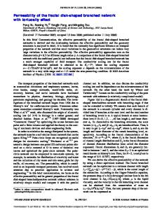
Fig. 2 Variation of return loss with frequency for base shape
v0 2 f r ε eff
− 2∆l
(4) Table 1 Frequencies at which minimum return loss occur for base shape
Where
v0
= Velocity of light in free space.
fr
= Operating resonant frequency.
εr
= Dielectric constant of the substrate used.
ε eff
= effective dielectric constant.
d
= height of the substrate.
Frequency
1.0 GHz
2.0 GHz
Return loss
-26.78 dB
-12.46 dB
The generalized formulas for iteration n are as follows: Nn = The number of black box. Ln = The ratio for length. An = The ratio for the fractal area after the nth iteration. n
= The iteration stage number. (a)
Nn = 8n
Ln =
1 3
An =
n
8 9
(5) n
(6)
3. RESULT AND DISSCUSSION
( b) Fig. 3
© 2011 JOT http://sites.google.com/site/journaloftelecommunications/
Radiation pattern at f =1.0GHz (a)
E-total, phi = 0(deg)
(b)
E-total, phi = 90(deg
JOURNAL OF TELECOMMUNICATIONS, VOLUME 8, ISSUE 2, MAY 2011 75
In figure2: the return loss -26.78 dB and -12.46 GHz with frequency 1.0GHz and 2.0 GHz respectively. The best return loss -26.78 dB ( 1GHz) was found.
(b) Fig. 5
Radiation pattern at f =0.87GHz (a)
E-total, phi = 0(deg)
(b)
E-total, phi = 90(deg
Fig. 4 Variation of return loss with frequency for first iteration.
Table 2 Frequencies at which minimum return loss occur for first iteration Frequency
0.87 GHz
1.87 GHz
2.19
(a)
GHz Return loss
-15.38 dB
-14.95 dB
-19.68 dB
(b)
Fig. 6
Radiation pattern at f =1.87 GHz (a)
E-total, phi = 0(deg)
(b) E-total, phi = 90(deg)
(a)
© 2011 JOT http://sites.google.com/site/journaloftelecommunications/
JOURNAL OF TELECOMMUNICATIONS, VOLUME 8, ISSUE 2, MAY 2011 76
Table 3 Frequencies at which minimum return loss occur for second iteration
Frequency
Return loss
0.85
1.83
2.13
2.68
GHz
GHz
GHz
GHz
-11.8
-12.89
-21.09
-14.17
dB
dB
dB
dB
(a)
(b) (a) Fig. 7
Radiation pattern at f =2.19GHz (a)
E-total, phi = 0(deg)
(b)
E-total, phi = 90(deg)
Figure 4 shows the result of return loss for first iteration. The resonant frequency was found at 0.87GHz, 1.87GHz and 2.19GHz from simulation. The best return loss -19.68dB (2.19GHz) was found.
(b)
Radiation pattern at f =0.85GHz
Fig. 9 (a)
E-total, phi = 0(deg)
(b)
E-total, phi = 90(deg)
Fig. 8 Variation of return loss with frequency for second iteration.
© 2011 JOT http://sites.google.com/site/journaloftelecommunications/
JOURNAL OF TELECOMMUNICATIONS, VOLUME 8, ISSUE 2, MAY 2011 77
(b)
(a)
Radiation pattern at f =2.13GHz
Fig. 11 (a)
E-total, phi = 0(deg)
(b) E-total, phi = 90(deg)
(b)
Fig. 10
Radiation pattern at f =1.83GHz (a)
E-total, phi = 0(deg)
(a)
(b) E-total, phi = 90(deg)
(b) (a) Radiation pattern at f =2.68GHz
Fig 12 (a)
E-total, phi = 0(deg)
(b)
E-total, phi = 90(deg)
Second iteration figure8 shows that four frequencies responses existed at 0.85GHz, 1.83GHz, 2.13GHz, and 2.68GHz. The best return loss at 2.13GHz(-21.09dB)..
© 2011 JOT http://sites.google.com/site/journaloftelecommunications/
JOURNAL OF TELECOMMUNICATIONS, VOLUME 8, ISSUE 2, MAY 2011 78
As the figure 12 illustrated, there were a side lobes existed at higher frequency. The side lobes occur at 2.72GHz.
Alok Nath Yadav B.Tech. (Electronics & comm.) from RGEC, Pusuing M.Tech.( Communication system) from Shobhit university, Meerut.
4. CONCLUSION The antenna has been simulated. The multiband frequencies appeared after applied fractal technique. It is observed that as the number of iterations is increased, number of frequency bands also increases. For zero iteration two bands occur, for first iteration three bands occur and for second iteration four bands occur. The antenna can be used for GPS, WLAN applications.
5. REFERENCES [1] Constantine A. Balanis, “Antenna Theory”, Second Edition, John Wiley & Son , 2000. [2] Abd M.F; Ja’afar A.S.: & Abd Aziz M.Z.A;” Sierpinski Carpet Fractal Antenna”, Proceedings of the 2007 AsiaPacific conference on applied electromagnetics, Melaka, December 2007.
Rajneesh Chawhan B.E. (Electronics) in 1997, M.Tech.(Digital Communication) in 2010 from U.P.T.U. & presently working as a Assistant Professor in Meerut Institute of Engineering & Technology, Meerut (India) affiliated by UPTU, Lucknow. Area of research interest include Antenna Designing, Microwave component designing, and written one book on Switching Theory with ISBN 8188476-29-X published by JPNP’s. Meerut , Prof. (Dr.) P.K. Singhal presently working as a Professor & Head in Department of Electronics Madhav Institute of Technology & Science, Gwalior and published lmore than hundred research paper, which include papers in IEEE transaction, International & National Journals, International and National Conference. Kumar Anubhav Tiwari presently working as a Assistant Professor in Shobhit University, Meerut.
[3] David M.Pozar, “Microstrip Antenna”, IEEE Transaction on Antenna and Propagation, January1992. [4] M.K. A. Rahim, N. Abdullah, and M.Z. A. Abdul Aziz, “Micro Strip Sierpinski Carpet Antenna Design” IEEE Transaction on Antenna and propagation,December 2005. [5] M.K. A.Rahim, N. Abdullah, and M.Z. A. Abdul Aziz, “Micro Strip Sierpinski Carpet Antenna using Transmission line Feeding”, IEEE Transaction on Antenna And Propagation, December 2005. [6] John Gianvittorio, “Fractal antennas: Design, Characterization, and Application”, Master Thesis, University of California, 2000. [7] B.B. Mandelbrot, “The Fractal Geometry of nature”, New York, W.H. Freeman, 1983. [8] Douglas H. Werner and Suman Ganguly.” An Overview of Fractal Engineering Research” , IEEE Antennas and Propagation Society, vol.45, no.1, pp.38-57, Feb 2003.
© 2011 JOT http://sites.google.com/site/journaloftelecommunications/