OTHER PLASTICITY MODELS
18.3
Other plasticity models
• • • • •
“Extended Drucker-Prager models,” Section 18.3.1 “Modified Drucker-Prager/Cap model,” Section 18.3.2 “Mohr-Coulomb plasticity,” Section 18.3.3 “Critical state (clay) plasticity model,” Section 18.3.4 “Crushable foam plasticity models,” Section 18.3.5
18.3–1
Abaqus Version 6.6 ID: Printed on:
DRUCKER-PRAGER
18.3.1
EXTENDED DRUCKER-PRAGER MODELS
Products: Abaqus/Standard
Abaqus/Explicit
Abaqus/CAE
References
• • • • • • • • • • •
“Material library: overview,” Section 16.1.1 “Inelastic behavior,” Section 18.1.1 “Rate-dependent yield,” Section 18.2.3 “Rate-dependent plasticity: creep and swelling,” Section 18.2.4 Chapter 19, “Progressive Damage and Failure” *DRUCKER PRAGER *DRUCKER PRAGER HARDENING *RATE DEPENDENT *DRUCKER PRAGER CREEP *TRIAXIAL TEST DATA “Defining Drucker-Prager plasticity” in “Defining plasticity,” Section 12.8.2 of the Abaqus/CAE User’s Manual, in the online HTML version of this manual
Overview
The extended Drucker-Prager models:
• • • • • • • •
are used to model frictional materials, which are typically granular-like soils and rock, and exhibit pressure-dependent yield (the material becomes stronger as the pressure increases); are used to model materials in which the compressive yield strength is greater than the tensile yield strength, such as those commonly found in composite and polymeric materials; allow a material to harden and/or soften isotropically; generally allow for volume change with inelastic behavior: the flow rule, defining the inelastic straining, allows simultaneous inelastic dilation (volume increase) and inelastic shearing; can include creep in Abaqus/Standard if the material exhibits long-term inelastic deformations; can be defined to be sensitive to the rate of straining, as is often the case in polymeric materials; can be used in conjunction with either the elastic material model (“Linear elastic behavior,” Section 17.2.1) or, in Abaqus/Standard if creep is not defined, the porous elastic material model (“Elastic behavior of porous materials,” Section 17.3.1); can be used in conjunction with the models of progressive damage and failure in Abaqus/Explicit (“Damage and failure for ductile metals: overview,” Section 19.2.1) to specify different damage initiation criteria and damage evolution laws that allow for the progressive degradation of the material stiffness and the removal of elements from the mesh; and
18.3.1–1
Abaqus Version 6.6 ID: Printed on:
DRUCKER-PRAGER
•
are intended to simulate material response under essentially monotonic loading.
Yield criteria
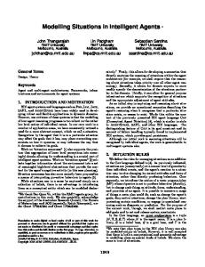
The yield criteria for this class of models are based on the shape of the yield surface in the meridional plane. The yield surface can have a linear form, a hyperbolic form, or a general exponent form. These surfaces are illustrated in Figure 18.3.1–1. t β
d
p a) Linear Drucker-Prager: F = t − p tan β − d = 0
β q
d −d /tanβ −pt
p
b) Hyperbolic: F = √(d |0 − pt |0 tan β) + q 2 − p tan β − d = 0 2
q
−pt
p
c) Exponent form: F = aq − p − pt = 0 b
Figure 18.3.1–1
Yield surfaces in the meridional plane.
18.3.1–2
Abaqus Version 6.6 ID: Printed on:
DRUCKER-PRAGER
The stress invariants and other terms in each of the three related yield criteria are defined later in this section. The linear model (Figure 18.3.1–1a) provides for a possibly noncircular yield surface in the deviatoric plane ( -plane) to match different yield values in triaxial tension and compression, associated inelastic flow in the deviatoric plane, and separate dilation and friction angles. Input data parameters define the shape of the yield and flow surfaces in the meridional and deviatoric planes as well as other characteristics of inelastic behavior such that a range of simple theories is provided—the original Drucker-Prager model is available within this model. However, this model cannot provide a close match to Mohr-Coulomb behavior, as described later in this section. The hyperbolic and general exponent models use a von Mises (circular) section in the deviatoric stress plane. In the meridional plane a hyperbolic flow potential is used for both models, which, in general, means nonassociated flow. The choice of model to be used depends largely on the analysis type, the kind of material, the experimental data available for calibration of the model parameters, and the range of pressure stress values that the material is likely to experience. It is common to have either triaxial test data at different levels of confining pressure or test data that are already calibrated in terms of a cohesion and a friction angle and, sometimes, a triaxial tensile strength value. If triaxial test data are available, the material parameters must be calibrated first. The accuracy with which the linear model can match these test data is limited by the fact that it assumes linear dependence of deviatoric stress on pressure stress. Although the hyperbolic model makes a similar assumption at high confining pressures, it provides a nonlinear relationship between deviatoric and pressure stress at low confining pressures, which may provide a better match of the triaxial experimental data. The hyperbolic model is useful for brittle materials for which both triaxial compression and triaxial tension data are available, which is a common situation for materials such as rocks. The most general of the three yield criteria is the exponent form. This criterion provides the most flexibility in matching triaxial test data. Abaqus determines the material parameters required for this model directly from the triaxial test data. A least-squares fit that minimizes the relative error in stress is used for this purpose. For cases where the experimental data are already calibrated in terms of a cohesion and a friction angle, the linear model can be used. If these parameters are provided for a Mohr-Coulomb model, it is necessary to convert them to Drucker-Prager parameters. The linear model is intended primarily for applications where the stresses are for the most part compressive. If tensile stresses are significant, hydrostatic tension data should be available (along with the cohesion and friction angle) and the hyperbolic model should be used. Calibration of these models is discussed later in this section. Hardening and rate dependence
For granular materials these models are often used as a failure surface, in the sense that the material can exhibit unlimited flow when the stress reaches yield. This behavior is called perfect plasticity. The models are also provided with isotropic hardening. In this case plastic flow causes the yield surface to change size uniformly with respect to all stress directions. This hardening model is useful for cases involving gross plastic straining or in which the straining at each point is essentially in the same direction
18.3.1–3
Abaqus Version 6.6 ID: Printed on:
DRUCKER-PRAGER
in strain space throughout the analysis. Although the model is referred to as an isotropic “hardening” model, strain softening, or hardening followed by softening, can be defined. As strain rates increase, many materials show an increase in their yield strength. This effect becomes important in many polymers when the strain rates range between 0.1 and 1 per second; it can be very important for strain rates ranging between 10 and 100 per second, which are characteristic of high-energy dynamic events or manufacturing processes. The effect is generally not as important in granular materials. The evolution of the yield surface with plastic deformation is described in terms of the equivalent stress , which can be chosen as either the uniaxial compression yield stress, the uniaxial tension yield stress, or the shear (cohesion) yield stress:
where is the equivalent plastic strain rate, defined for the linear Drucker-Prager model as = if hardening is defined in uniaxial compression; = =
if hardening is defined in uniaxial tension; if hardening is defined in pure shear,
and defined for the hyperbolic and exponential Drucker-Prager models as
is the equivalent plastic strain; is temperature; and are other predefined field variables. includes hardening as well as rate-dependent effects. The functional dependence The material data can be input either directly in a tabular format or by correlating it to static relations based on yield stress ratios. Rate dependence as described here is most suitable for moderate- to high-speed events in Abaqus/Standard. Time-dependent inelastic deformation at low deformation rates can be better represented by creep models. Such inelastic deformation, which can coexist with rate-independent plastic deformation, is described later in this section. However, the existence of creep in an Abaqus/Standard material definition precludes the use of rate dependence as described here.
18.3.1–4
Abaqus Version 6.6 ID: Printed on:
DRUCKER-PRAGER
When using the Drucker-Prager material model, Abaqus allows you to prescribe initial hardening by defining initial equivalent plastic strain values, as discussed below along with other details regarding the use of initial conditions. Direct tabular data
Test data are entered as tables of yield stress values versus equivalent plastic strain at different equivalent plastic strain rates; one table per strain rate. Compression data are more commonly available for geological materials, whereas tension data are usually available for polymeric materials. The guidelines on how to enter these data are provided in “Rate-dependent yield,” Section 18.2.3. Input File Usage: Abaqus/CAE Usage:
*DRUCKER PRAGER HARDENING, RATE= Property module: material editor: Mechanical→Plasticity→Drucker Prager: Suboptions→Drucker Prager Hardening: toggle on Use strain-rate-dependent data
Yield stress ratios
Alternatively, the strain rate behavior can be assumed to be separable, so that the stress-strain dependence is similar at all strain rates:
where is the static stress-strain behavior and is the ratio of the yield stress at nonzero strain rate to the static yield stress (so that ). Two methods are offered to define R in Abaqus: specifying an overstress power law or defining the variable R directly as a tabular function of . Overstress power law
The Cowper-Symonds overstress power law has the form
where and are material parameters that can be functions of temperature and, possibly, of other predefined field variables. Input File Usage:
Use both of the following options:
Abaqus/CAE Usage:
*DRUCKER PRAGER HARDENING *RATE DEPENDENT, TYPE=POWER LAW Property module: material editor: Mechanical→Plasticity→Drucker Prager: Suboptions→Drucker Prager Hardening; Suboptions→Rate Dependent: Hardening: Power Law
18.3.1–5
Abaqus Version 6.6 ID: Printed on:
DRUCKER-PRAGER
Tabular function
When R is entered directly, it is entered as a tabular function of the equivalent plastic strain rate, temperature, ; and predefined field variables, . Input File Usage:
Use both of the following options:
Abaqus/CAE Usage:
*DRUCKER PRAGER HARDENING *RATE DEPENDENT, TYPE=YIELD RATIO Property module: material editor: Mechanical→Plasticity→Drucker Prager: Suboptions→Drucker Prager Hardening; Suboptions→Rate Dependent: Hardening: Yield Ratio
;
Stress invariants
The yield stress surface makes use of two invariants, defined as the equivalent pressure stress,
and the Mises equivalent stress,
where
is the stress deviator, defined as
In addition, the linear model also uses the third invariant of deviatoric stress,
Linear Drucker-Prager model
The linear model is written in terms of all three stress invariants. It provides for a possibly noncircular yield surface in the deviatoric plane to match different yield values in triaxial tension and compression, associated inelastic flow in the deviatoric plane, and separate dilation and friction angles. Yield criterion
The linear Drucker-Prager criterion (see Figure 18.3.1–1a) is written as
where
18.3.1–6
Abaqus Version 6.6 ID: Printed on:
DRUCKER-PRAGER
is the slope of the linear yield surface in the p–t stress plane and is commonly referred to as the friction angle of the material; is the cohesion of the material; and
d
is the ratio of the yield stress in triaxial tension to the yield stress in triaxial compression and, thus, controls the dependence of the yield surface on the value of the intermediate principal stress (see Figure 18.3.1–2).
S3
1 q 1+ _ 1 - 1- _ 1 t= _ 2 K K
)
b
a
K
a
1.0
b
0.8
3
S2
S1
Figure 18.3.1–2
Curve
) _r ) )q
Typical yield/flow surfaces of the linear model in the deviatoric plane.
In the case of hardening defined in uniaxial compression, the linear yield criterion precludes friction angles 71.5° ( 3), which is unlikely to be a limitation for real materials. , , which implies that the yield surface is the von Mises circle in the deviatoric When principal stress plane (the -plane), in which case the yield stresses in triaxial tension and compression are the same. To ensure that the yield surface remains convex requires . The cohesion, d, of the material is related to the input data as
18.3.1–7
Abaqus Version 6.6 ID: Printed on:
DRUCKER-PRAGER
Plastic flow
G is the flow potential, chosen in this model as
where is the dilation angle in the p–t plane. A geometric interpretation of is shown in the p–t diagram of Figure 18.3.1–3. In the case of hardening defined in uniaxial compression, this flow rule definition precludes dilation angles 71.5° ( 3). This restriction is not seen as a limitation since it is unlikely this will be the case for real materials. pl
dε
ψ t β hardening β d p
Figure 18.3.1–3 Linear Drucker-Prager model: yield surface and flow direction in the p–t plane. For granular materials the linear model is normally used with nonassociated flow in the p–t plane, in the sense that the flow is assumed to be normal to the yield surface in the -plane but at an angle to the t-axis in the p–t plane, where usually , as illustrated in Figure 18.3.1–3. Associated flow results from setting . The original Drucker-Prager model is available by setting and . Nonassociated flow is also generally assumed when the model is used for polymeric materials. If , the inelastic deformation is incompressible; if , the material dilates. Hence, is referred to as the dilation angle. The relationship between the flow potential and the incremental plastic strain for the linear model is discussed in detail in “Models for granular or polymer behavior,” Section 4.4.2 of the Abaqus Theory Manual.
18.3.1–8
Abaqus Version 6.6 ID: Printed on:
DRUCKER-PRAGER
*DRUCKER PRAGER, SHEAR CRITERION=LINEAR Property module: material editor: Mechanical→Plasticity→Drucker Prager: Shear criterion: Linear
Input File Usage: Abaqus/CAE Usage:
Nonassociated flow
Nonassociated flow implies that the material stiffness matrix is not symmetric; therefore, the unsymmetric matrix storage and solution scheme should be used in Abaqus/Standard (see “Procedures: overview,” Section 6.1.1). If the difference between and is not large and the region of the model in which inelastic deformation is occurring is confined, it is possible that a symmetric approximation to the material stiffness matrix will give an acceptable rate of convergence and the unsymmetric matrix scheme may not be needed. Hyperbolic and general exponent models
The hyperbolic and general exponent models available are written in terms of the first two stress invariants only. Hyperbolic yield criterion
The hyperbolic yield criterion is a continuous combination of the maximum tensile stress condition of Rankine (tensile cut-off) and the linear Drucker-Prager condition at high confining stress. It is written as
where
and is the initial hydrostatic tension strength of the material; is the hardening parameter; is the initial value of ; and is the friction angle measured at high confining pressure, as shown in Figure 18.3.1–1(b).
The hardening parameter,
, can be obtained from test data as follows:
The isotropic hardening assumed in this model treats Figure 18.3.1–4.
18.3.1–9
Abaqus Version 6.6 ID: Printed on:
as constant with respect to stress as depicted in
DRUCKER-PRAGER
hardening q
β
p l0/tanβ
Figure 18.3.1–4 Input File Usage: Abaqus/CAE Usage:
l0/tanβ
l0/tanβ
Hyperbolic model: yield surface and hardening in the p–q plane. *DRUCKER PRAGER, SHEAR CRITERION=HYPERBOLIC Property module: material editor: Mechanical→Plasticity→Drucker Prager: Shear criterion: Hyperbolic
General exponent yield criterion
The general exponent form provides the most general yield criterion available in this class of models. The yield function is written as
where and
are material parameters that are independent of plastic deformation; and is the hardening parameter that represents the hydrostatic tension strength of the material as shown in Figure 18.3.1–1(c).
is related to the input test data as
The isotropic hardening assumed in this model treats a and b as constant with respect to stress, as depicted in Figure 18.3.1–5.
18.3.1–10
Abaqus Version 6.6 ID: Printed on:
DRUCKER-PRAGER
hardening
( pat
1/b
)
q
p
pt Figure 18.3.1–5
General exponent model: yield surface and hardening in the p–q plane.
The material parameters a and b can be given directly. Alternatively, if triaxial test data at different levels of confining pressure are available, Abaqus will determine the material parameters from the triaxial test data, as discussed below. Input File Usage: Abaqus/CAE Usage:
*DRUCKER PRAGER, SHEAR CRITERION=EXPONENT FORM Property module: material editor: Mechanical→Plasticity→Drucker Prager: Shear criterion: Exponent Form
Plastic flow
G is the flow potential, chosen in these models as a hyperbolic function:
where is the dilation angle measured in the p–q plane at high confining pressure; is the initial yield stress, taken from the user-specified DruckerPrager hardening data; and is a parameter, referred to as the eccentricity, that defines the rate at which the function approaches the asymptote (the flow potential tends to a straight line as the eccentricity tends to zero). Suitable default values are provided for , as described below. The value of will depend on the yield stress used. This flow potential, which is continuous and smooth, ensures that the flow direction is always uniquely defined. The function approaches the linear Drucker-Prager flow potential asymptotically at high confining pressure stress and intersects the hydrostatic pressure axis at 90°. A family of hyperbolic
18.3.1–11
Abaqus Version 6.6 ID: Printed on:
DRUCKER-PRAGER
potentials in the meridional stress plane is shown in Figure 18.3.1–6. The flow potential is the von Mises circle in the deviatoric stress plane (the -plane).
dε
pl
ψ
q
p
σ |0
∋
Figure 18.3.1–6
Family of hyperbolic flow potentials in the p–q plane.
For the hyperbolic model flow is nonassociated in the p–q plane if the dilation angle, , and the material friction angle, , are different. The hyperbolic model provides associated flow in the p–q plane only when and . A default value of ) is assumed if the flow potential is used with the hyperbolic model, so that associated flow is recovered when . For the general exponent model flow is always nonassociated in the p–q plane. The default flow potential eccentricity is , which implies that the material has almost the same dilation angle over a wide range of confining pressure stress values. Increasing the value of provides more curvature to the flow potential, implying that the dilation angle increases more rapidly as the confining pressure decreases. Values of that are significantly less than the default value may lead to convergence problems if the material is subjected to low confining pressures because of the very tight curvature of the flow potential locally where it intersects the p-axis. The relationship between the flow potential and the incremental plastic strain for the hyperbolic and general exponent models is discussed in detail in “Models for granular or polymer behavior,” Section 4.4.2 of the Abaqus Theory Manual. Nonassociated flow
Nonassociated flow implies that the material stiffness matrix is not symmetric; therefore, the unsymmetric matrix storage and solution scheme should be used in Abaqus/Standard (see “Procedures: overview,” Section 6.1.1). If the difference between and in the hyperbolic model is not large and if the region of the model in which inelastic deformation is occurring is confined, it is possible that a symmetric approximation to the material stiffness matrix will give an acceptable rate of convergence. In such cases the unsymmetric matrix scheme may not be needed.
18.3.1–12
Abaqus Version 6.6 ID: Printed on:
DRUCKER-PRAGER
Progressive damage and failure
In Abaqus/Explicit the extended Drucker-Prager models can be used in conjunction with the models of progressive damage and failure discussed in “Damage and failure for ductile metals: overview,” Section 19.2.1. The capability allows for the specification of one or more damage initiation criteria, including ductile, shear, forming limit diagram (FLD), forming limit stress diagram (FLSD), and Müschenborn-Sonne forming limit diagram (MSFLD) criteria. After damage initiation, the material stiffness is degraded progressively according to the specified damage evolution response. The model offers two failure choices, including the removal of elements from the mesh as a result of tearing or ripping of the structure. The progressive damage models allow for a smooth degradation of the material stiffness, making them suitable for both quasi-static and dynamic situations. Input File Usage:
Use the following options:
Abaqus/CAE Usage:
*DAMAGE INITIATION *DAMAGE EVOLUTION Property module: material editor: Mechanical→Damage for Ductile Metals→damage initiation type: specify the damage initiation criterion: Suboptions→Damage Evolution: specify the damage evolution parameters
Matching experimental triaxial test data
Data for geological materials are most commonly available from triaxial testing. In such a test the specimen is confined by a pressure stress that is held constant during the test. The loading is an additional tension or compression stress applied in one direction. Typical results include stress-strain curves at different levels of confinement, as shown in Figure 18.3.1–7. To calibrate the yield parameters for this class of models, you need to decide which point on each stress-strain curve will be used for calibration. For example, if you wish to calibrate the initial yield surface, the point in each stress-strain curve corresponding to initial deviation from elastic behavior should be used. Alternatively, if you wish to calibrate the ultimate yield surface, the point in each stress-strain curve corresponding to the peak stress should be used. One stress data point from each stress-strain curve at a different level of confinement is plotted in the meridional stress plane (p–t plane if the linear model is to be used, or p–q plane if the hyperbolic or general exponent model will be used). This technique calibrates the shape and position of the yield surface, as shown in Figure 18.3.1–8, and is adequate to define a model if it is to be used as a failure surface (perfect plasticity). The models are also available with isotropic hardening, in which case hardening data are required to complete the calibration. In an isotropic hardening model plastic flow causes the yield surface to change size uniformly; in other words, only one of the stress-strain curves depicted in Figure 18.3.1–7 can be used to represent hardening. The curve that represents hardening most accurately over the range of loading conditions anticipated should be selected (usually the curve for the average anticipated value of pressure stress). As stated earlier, two types of triaxial test data are commonly available for geological materials. In a triaxial compression test the specimen is confined by pressure and an additional compression stress is superposed in one direction. Thus, the principal stresses are all negative, with
18.3.1–13
Abaqus Version 6.6 ID: Printed on:
DRUCKER-PRAGER
σ3
points chosen to define shape and position of yield surface
-σ3 increasing confinement
-σ2
-σ1
ε3
Figure 18.3.1–7 Triaxial tests with stress-strain curves for typical geological materials at different levels of confinement. q
p
Figure 18.3.1–8
Yield surface in meridional plane.
(Figure 18.3.1–9a). In the preceding inequality minimum principal stresses, respectively. The values of the stress invariants are
,
and
18.3.1–14
Abaqus Version 6.6 ID: Printed on:
, and
are the maximum, intermediate, and
DRUCKER-PRAGER
-σ3
-σ1
σ1= σ2 ≥ σ3
-σ2
-σ1
σ1 ≥ σ2 = σ3
a Figure 18.3.1–9
-σ3
-σ2
b a) Triaxial compression and b) tension.
so that
The triaxial compression results can, thus, be plotted in the meridional plane shown in Figure 18.3.1–8. Linear Drucker-Prager model
Fitting the best straight line through the triaxial compression results provides and d for the linear Drucker-Prager model. Triaxial tension data are also needed to define K in the linear Drucker-Prager model. Under triaxial tension the specimen is again confined by pressure, after which the pressure in one direction is reduced. In this case the principal stresses are (Figure 18.3.1–9b). The stress invariants are now
and
so that
18.3.1–15
Abaqus Version 6.6 ID: Printed on:
DRUCKER-PRAGER
Thus, K can be found by plotting these test results as q versus p and again fitting the best straight line. The triaxial compression and tension lines must intercept the p-axis at the same point, and the ratio of values of q for triaxial tension and compression at the same value of p then gives K (Figure 18.3.1–10). q
Best fit to triaxial compression data Best fit to triaxial tension data
qc β
qt
qt =K qc
d p
Figure 18.3.1–10
Linear model: fitting triaxial compression and tension data.
Hyperbolic model
Fitting the best straight line through the triaxial compression results at high confining pressures provides and for the hyperbolic model. This fit is performed in the same manner as that used to obtain and d for the linear Drucker-Prager model. In addition, hydrostatic tension data are required to complete the calibration of the hyperbolic model so that the initial hydrostatic tension strength, , can be defined. General exponent model
Given triaxial data in the meridional plane, Abaqus provides a capability to determine the material parameters a, b, and required for the exponent model. The parameters are determined on the basis of a “best fit” of the triaxial test data at different levels of confining stress. A least-squares fit which minimizes the relative error in stress is used to obtain the “best fit” values for a, b, and . The capability allows all three parameters to be calibrated or, if some of the parameters are known, only the remaining parameters to be calibrated. This ability is useful if only a few data points are available, in which case you may wish to fit the best straight line ( ) through the data points (effectively reducing the model to a linear Drucker-Prager model). Partial calibration can also be useful in a case when triaxial test data
18.3.1–16
Abaqus Version 6.6 ID: Printed on:
DRUCKER-PRAGER
at low confinement are unreliable or unavailable, as is often the case for cohesionless materials. In this case a better fit may be obtained if the value of is specified and only a and b are calibrated. The data must be provided in terms of the principal stresses and , where is the confining stress and is the stress in the loading direction. The Abaqus sign convention must be followed such that tensile stresses are positive and compressive stresses are negative. One pair of stresses must be entered from each triaxial test. As many data points as desired can be entered from triaxial tests at different levels of confining stress. If the exponent model is used as a failure surface (perfect plasticity), the Drucker-Prager hardening behavior does not have to be specified. The hydrostatic tension strength, , obtained from the calibration will then be used as the failure stress. However, if the Drucker-Prager hardening behavior is specified together with the triaxial test data, the value of obtained from the calibration will be ignored. In this case Abaqus will interpolate directly from the hardening data. Input File Usage:
Abaqus/CAE Usage:
Use both of the following options: *DRUCKER PRAGER, SHEAR CRITERION=EXPONENT FORM, TEST DATA *TRIAXIAL TEST DATA Property module: material editor: Mechanical→Plasticity→Drucker Prager: Shear criterion: Exponent Form, toggle on Use Suboption Triaxial Test Data, and select Suboptions→Triaxial Test Data
Matching Mohr-Coulomb parameters to the Drucker-Prager model
Sometimes experimental data are not directly available. Instead, you are provided with the friction angle and cohesion values for the Mohr-Coulomb model. In that case the simplest way to proceed in Abaqus/Standard is to use the Mohr-Coulomb model (see “Mohr-Coulomb plasticity,” Section 18.3.3). In some situations it may be necessary to use the Drucker-Prager model instead of the Mohr-Coulomb model (such as when rate effects need to be considered), in which case we need to calculate values for the parameters of a Drucker-Prager model to provide a reasonable match to the Mohr-Coulomb parameters. The Mohr-Coulomb failure model is based on plotting Mohr’s circle for states of stress at failure in the plane of the maximum and minimum principal stresses. The failure line is the best straight line that touches these Mohr’s circles (Figure 18.3.1–11). Therefore, the Mohr-Coulomb model is defined by
where
is negative in compression. From Mohr’s circle,
Substituting for can be written as
and , multiplying both sides by
18.3.1–17
Abaqus Version 6.6 ID: Printed on:
, and reducing, the Mohr-Coulomb model
DRUCKER-PRAGER
τ
s= φ
σ1 - σ3 2
c σ1 σm=
σ3
σ1
σ3
σ (compressive stress)
σ1+σ3 2
Figure 18.3.1–11
Mohr-Coulomb failure model.
where
is half of the difference between the maximum principal stress, (and is, therefore, the maximum shear stress),
, and the minimum principal stress,
is the average of the maximum and minimum principal stresses, and is the friction angle. Thus, the model assumes a linear relationship between deviatoric and pressure stress and, so, can be matched by the linear or hyperbolic Drucker-Prager models provided in Abaqus. The Mohr-Coulomb model assumes that failure is independent of the value of the intermediate principal stress, but the Drucker-Prager model does not. The failure of typical geotechnical materials generally includes some small dependence on the intermediate principal stress, but the Mohr-Coulomb model is generally considered to be sufficiently accurate for most applications. This model has vertices in the deviatoric plane (see Figure 18.3.1–12). The implication is that, whenever the stress state has two equal principal stress values, the flow direction can change significantly with little or no change in stress. None of the models currently available in Abaqus can provide such behavior; even in the Mohr-Coulomb model the flow potential is smooth. This limitation is generally not a key concern in many design calculations involving
18.3.1–18
Abaqus Version 6.6 ID: Printed on:
DRUCKER-PRAGER
S3 Mohr-Coulomb
S2
S1
Drucker-Prager
Figure 18.3.1–12
Mohr-Coulomb model in the deviatoric plane.
Coulomb-like materials, but it can limit the accuracy of the calculations, especially in cases where flow localization is important. Matching plane strain response
Plane strain problems are often encountered in geotechnical analysis; for example, long tunnels, footings, and embankments. Therefore, the constitutive model parameters are often matched to provide the same flow and failure response in plane strain. The matching procedure described below is carried out in terms of the linear Drucker-Prager model but is also applicable to the hyperbolic model at high levels of confining stress. The linear Drucker-Prager flow potential defines the plastic strain increment as
where is the equivalent plastic strain increment. Since we wish to match the behavior in only one plane, we can take , which implies that . Thus,
Writing this expression in terms of principal stresses provides
18.3.1–19
Abaqus Version 6.6 ID: Printed on:
DRUCKER-PRAGER
with similar expressions for and . Assume plane strain in the 1-direction. At limit load we must have , which provides the constraint
Using this constraint we can rewrite q and p in terms of the principal stresses in the plane of deformation, and , as
and
With these expressions the Drucker-Prager yield surface can be written in terms of
The Mohr-Coulomb yield surface in the
and
as
plane is
By comparison,
These relationships provide a match between the Mohr-Coulomb material parameters and linear Drucker-Prager material parameters in plane strain. Consider the two extreme cases of flow definition: associated flow, , and nondilatant flow, when . For associated flow and and for nondilatant flow and
18.3.1–20
Abaqus Version 6.6 ID: Printed on:
DRUCKER-PRAGER
In either case
is immediately available as
The difference between these two approaches increases with the friction angle; however, the results are not very different for typical friction angles, as illustrated in Table 18.3.1–1. Table 18.3.1–1
Plane strain matching of Drucker-Prager and Mohr-Coulomb models.
Mohr-Coulomb friction angle,
Associated flow Drucker-Prager friction angle,
Nondilatant flow Drucker-Prager friction angle,
10°
16.7°
1.70
16.7°
1.70
20°
30.2°
1.60
30.6°
1.63
30°
39.8°
1.44
40.9°
1.50
40°
46.2°
1.24
48.1°
1.33
50°
50.5°
1.02
53.0°
1.11
“Limit load calculations with granular materials,” Section 1.14.4 of the Abaqus Benchmarks Manual, and “Finite deformation of an elastic-plastic granular material,” Section 1.14.5 of the Abaqus Benchmarks Manual, show a comparison of the response of a simple loading of a granular material using the Drucker-Prager and Mohr-Coulomb models, using the plane strain approach to match the parameters of the two models. Matching triaxial test response
Another approach to matching Mohr-Coulomb and Drucker-Prager model parameters for materials with low friction angles is to make the two models provide the same failure definition in triaxial compression and tension. The following matching procedure is applicable only to the linear Drucker-Prager model since this is the only model in this class that allows for different yield values in triaxial compression and tension. We can rewrite the Mohr-Coulomb model in terms of principal stresses:
Using the results above for the stress invariants p, q, and r in triaxial compression and tension allows the linear Drucker-Prager model to be written for triaxial compression as
18.3.1–21
Abaqus Version 6.6 ID: Printed on:
DRUCKER-PRAGER
and for triaxial tension as
We wish to make these expressions identical to the Mohr-Coulomb model for all values of This is possible by setting
.
By comparing the Mohr-Coulomb model with the linear Drucker-Prager model,
and, hence, from the previous result
These results for and provide linear Drucker-Prager parameters that match the MohrCoulomb model in triaxial compression and tension. The value of K in the linear Drucker-Prager model is restricted to for the yield surface to remain convex. The result for K shows that this implies . Many real materials have a larger Mohr-Coulomb friction angle than this value. One approach in such circumstances is to choose and then to use the remaining equations to define and . This approach matches the models for triaxial compression only, while providing the closest approximation that the model can provide to failure being independent of the intermediate principal stress. If is significantly larger than 22°, this approach may provide a poor Drucker-Prager match of the Mohr-Coulomb parameters. Therefore, this matching procedure is not generally recommended; in Abaqus/Standard use the Mohr-Coulomb model instead. While using one-element tests to verify the calibration of the model, it should be noted that the Abaqus output variables SP1, SP2, and SP3 correspond to the principal stresses , , and , respectively. Creep models for the linear Drucker-Prager model
Classical “creep” behavior of materials that exhibit plasticity according to the extended Drucker-Prager models can be defined in Abaqus/Standard. The creep behavior in such materials is intimately tied to the plasticity behavior (through the definitions of creep flow potentials and definitions of test data), so Drucker-Prager plasticity and Drucker-Prager hardening must be included in the material definition.
18.3.1–22
Abaqus Version 6.6 ID: Printed on:
DRUCKER-PRAGER
Creep and plasticity can be active simultaneously, in which case the resulting equations are solved in a coupled manner. To model creep only (without rate-independent plastic deformation), large values for the yield stress should be provided in the Drucker-Prager hardening definition: the result is that the material follows the Drucker-Prager model while it creeps, without ever yielding. When using this technique, a value must also be defined for the eccentricity, since, as described below, both the initial yield stress and eccentricity affect the creep potentials. This capability is limited to the linear model with a von Mises (circular) section in the deviatoric stress plane ( ; i.e., no third stress invariant effects are taken into account) and can be combined only with linear elasticity. Creep behavior defined by the extended Drucker-Prager model is active only during soils consolidation, coupled temperature-displacement, and transient quasi-static procedures. Creep formulation
The creep potential is hyperbolic, similar to the plastic flow potentials used in the hyperbolic and general exponent plasticity models. If creep properties are defined in Abaqus/Standard, the linear Drucker-Prager plasticity model also uses a hyperbolic plastic flow potential. As a consequence, if two analyses are run, one in which creep is not activated and another in which creep properties are specified but produce virtually no creep flow, the plasticity solutions will not be exactly the same: the solution with creep not activated uses a linear plastic potential, whereas the solution with creep activated uses a hyperbolic plastic potential. Equivalent creep surface and equivalent creep stress
We adopt the notion of the existence of creep isosurfaces of stress points that share the same creep “intensity,” as measured by an equivalent creep stress. When the material plastifies, it is desirable to have the equivalent creep surface coincide with the yield surface; therefore, we define the equivalent creep surfaces by homogeneously scaling down the yield surface. In the p–q plane that translates into parallels to the yield surface, as depicted in Figure 18.3.1–13. Abaqus/Standard requires that creep properties be described in terms of the same type of data used to define work hardening properties. The equivalent creep stress, , is then determined as follows:
Figure 18.3.1–13 shows how the equivalent point is determined when the material properties are in shear, with stress d. A consequence of these concepts is that there is a cone in p–q space inside which creep is not active since any point inside this cone would have a negative equivalent creep stress.
18.3.1–23
Abaqus Version 6.6 ID: Printed on:
DRUCKER-PRAGER
q
yield surface
β
material point
equivalent creep surface
σ−cr no creep
p
Figure 18.3.1–13
Equivalent creep stress defined as the shear stress.
Creep flow
The creep strain rate in Abaqus/Standard is assumed to follow from the same hyperbolic potential as the plastic strain rate (see Figure 18.3.1–6):
where is the dilation angle measured in the p–q plane at high confining pressure; is the initial yield stress taken from the user-specified DruckerPrager hardening data; and is a parameter, referred to as the eccentricity, that defines the rate at which the function approaches the asymptote (the creep potential tends to a straight line as the eccentricity tends to zero). Suitable default values are provided for , as described below. This creep potential, which is continuous and smooth, ensures that the creep flow direction is always uniquely defined. The function approaches the linear Drucker-Prager flow potential asymptotically at high confining pressure stress and intersects the hydrostatic pressure axis at 90°. A family of hyperbolic potentials in the meridional stress plane was shown in Figure 18.3.1–6. The creep potential is the von Mises circle in the deviatoric stress plane (the -plane). The default creep potential eccentricity is , which implies that the material has almost the same dilation angle over a wide range of confining pressure stress values. Increasing the value of provides more curvature to the creep potential, implying that the dilation angle increases as the confining pressure decreases. Values of that are significantly less than the default value may lead to convergence
18.3.1–24
Abaqus Version 6.6 ID: Printed on:
DRUCKER-PRAGER
problems if the material is subjected to low confining pressures, because of the very tight curvature of the creep potential locally where it intersects the p-axis. For details on the behavior of these models refer to “Verification of creep integration,” Section 3.2.6 of the Abaqus Benchmarks Manual. If the creep material properties are defined by a compression test, numerical problems may arise for very low stress values. Abaqus/Standard protects for such a case, as described in “Models for granular or polymer behavior,” Section 4.4.2 of the Abaqus Theory Manual. Nonassociated flow
The use of a creep potential different from the equivalent creep surface implies that the material stiffness matrix is not symmetric; therefore, the unsymmetric matrix storage and solution scheme should be used (see “Procedures: overview,” Section 6.1.1). If the difference between and is not large and the region of the model in which inelastic deformation is occurring is confined, it is possible that a symmetric approximation to the material stiffness matrix will give an acceptable rate of convergence and the unsymmetric matrix scheme may not be needed. Specifying a creep law
The definition of creep behavior in Abaqus/Standard is completed by specifying the equivalent “uniaxial behavior”—the creep “law.” In many practical cases the creep “law” is defined through user subroutine CREEP because creep laws are usually of very complex form to fit experimental data. Data input methods are provided for some simple cases, including two forms of a power law model and a variation of the Singh-Mitchell law. User subroutine CREEP
User subroutine CREEP provides a very general capability for implementing viscoplastic models in Abaqus/Standard in which the strain rate potential can be written as a function of the equivalent stress and any number of “solution-dependent state variables.” When used in conjunction with these material models, the equivalent creep stress, , is made available in the routine. Solution-dependent state variables are any variables that are used in conjunction with the constitutive definition and whose values evolve with the solution. Examples are hardening variables associated with the model. When a more general form is required for the stress potential, user subroutine UMAT can be used. Input File Usage: Abaqus/CAE Usage:
*DRUCKER PRAGER CREEP, LAW=USER Property module: material editor: Mechanical→Plasticity→Drucker Prager: Suboptions→Drucker Prager Creep: Law: User
“Time hardening” form of the power law model
The “time hardening” form of the power law model is
where
18.3.1–25
Abaqus Version 6.6 ID: Printed on:
DRUCKER-PRAGER
t A, n, and m Input File Usage: Abaqus/CAE Usage:
is the equivalent creep strain rate, defined so that if the equivalent creep stress is defined in uniaxial compression, if defined in uniaxial tension, and if defined in pure shear, where is the engineering shear creep strain; is the equivalent creep stress; is the total time; and are user-defined creep material parameters specified as functions of temperature and field variables. *DRUCKER PRAGER CREEP, LAW=TIME Property module: material editor: Mechanical→Plasticity→Drucker Prager: Suboptions→Drucker Prager Creep: Law: Time
“Strain hardening” form of the power law model
As an alternative to the “time hardening” form of the power law, as defined above, the corresponding “strain hardening” form can be used:
For physically reasonable behavior A and n must be positive and Input File Usage: Abaqus/CAE Usage:
.
*DRUCKER PRAGER CREEP, LAW=STRAIN Property module: material editor: Mechanical→Plasticity→Drucker Prager: Suboptions→Drucker Prager Creep: Law: Strain
Singh-Mitchell law
A second creep law available as data input is a variation of the Singh-Mitchell law:
where , t, and are defined above and A, , , and m are user-defined creep material parameters specified as functions of temperature and field variables. For physically reasonable behavior A and must be positive, , and should be small compared to the total time. Input File Usage: Abaqus/CAE Usage:
*DRUCKER PRAGER CREEP, LAW=SINGHM Property module: material editor: Mechanical→Plasticity→Drucker Prager: Suboptions→Drucker Prager Creep: Law: SinghM
Numerical difficulties
Depending on the choice of units for the creep laws described above, the value of A may be very small for typical creep strain rates. If A is less than , numerical difficulties can cause errors in the material calculations; therefore, use another system of units to avoid such difficulties in the calculation of creep strain increments.
18.3.1–26
Abaqus Version 6.6 ID: Printed on:
DRUCKER-PRAGER
Creep integration
Abaqus/Standard provides both explicit and implicit time integration of creep and swelling behavior. The choice of the time integration scheme depends on the procedure type, the parameters specified for the procedure, the presence of plasticity, and whether or not a geometric linear or nonlinear analysis is requested, as discussed in “Rate-dependent plasticity: creep and swelling,” Section 18.2.4. Initial conditions
There are cases when we need to study the behavior of a material that has already been subjected to some work hardening. For such cases Abaqus allows you to prescribe initial conditions for the equivalent plastic strain, , by specifying the conditions directly (see “Initial conditions,” Section 27.2.1). For more complicated cases initial conditions can be defined in Abaqus/Standard through user subroutine HARDINI. Use the following option to specify the initial equivalent plastic strain directly:
Input File Usage:
*INITIAL CONDITIONS, TYPE=HARDENING Use the following option in Abaqus/Standard to specify the initial equivalent plastic strain in user subroutine HARDINI: Abaqus/CAE Usage:
*INITIAL CONDITIONS, TYPE=HARDENING, USER Initial hardening conditions are not supported in Abaqus/CAE.
Elements
The Drucker-Prager models can be used with the following element types: plane strain, generalized plane strain, axisymmetric, and three-dimensional solid (continuum) elements. All Drucker-Prager models are also available in plane stress (plane stress, shell, and membrane elements), except for the linear DruckerPrager model with creep. Output
In addition to the standard output identifiers available in Abaqus (“Abaqus/Standard output variable identifiers,” Section 4.2.1, and “Abaqus/Explicit output variable identifiers,” Section 4.2.2), the following variables have special meaning for the Drucker-Prager plasticity/creep model: PEEQ
CEEQ
Equivalent plastic strain. For the linear Drucker-Prager plasticity model PEEQ is defined as ; where is the initial equivalent plastic strain (zero or user-specified; is the equivalent plastic strain rate. see “Initial conditions”) and For the hyperbolic and exponential Drucker-Prager plasticity models PEEQ is defined as , where is the initial equivalent plastic strain and is the yield stress. . Equivalent creep strain,
18.3.1–27
Abaqus Version 6.6 ID: Printed on:
CAP MODEL
18.3.2
MODIFIED DRUCKER-PRAGER/CAP MODEL
Products: Abaqus/Standard
Abaqus/Explicit
Abaqus/CAE
References
• • • • • • • •
“Inelastic behavior,” Section 18.1.1 “Material library: overview,” Section 16.1.1 “Rate-dependent plasticity: creep and swelling,” Section 18.2.4 “CREEP,” Section 1.1.1 of the Abaqus User Subroutines Reference Manual *CAP PLASTICITY *CAP HARDENING *CAP CREEP “Defining cap plasticity” in “Defining plasticity,” Section 12.8.2 of the Abaqus/CAE User’s Manual, in the online HTML version of this manual
Overview
The modified Drucker-Prager/Cap plasticity/creep model:
• •
• • •
is intended to model cohesive geological materials that exhibit pressure-dependent yield, such as soils and rocks; is based on the addition of a cap yield surface to the Drucker-Prager plasticity model (“Extended Drucker-Prager models,” Section 18.3.1), which provides an inelastic hardening mechanism to account for plastic compaction and helps to control volume dilatancy when the material yields in shear; can be used in Abaqus/Standard to simulate creep in materials exhibiting long-term inelastic deformation through a cohesion creep mechanism in the shear failure region and a consolidation creep mechanism in the cap region; can be used in conjunction with either the elastic material model (“Linear elastic behavior,” Section 17.2.1) or, in Abaqus/Standard if creep is not defined, the porous elastic material model (“Elastic behavior of porous materials,” Section 17.3.1); and provides a reasonable response to large stress reversals in the cap region; however, in the failure surface region the response is reasonable only for essentially monotonic loading.
Yield surface
The addition of the cap yield surface to the Drucker-Prager model serves two main purposes: it bounds the yield surface in hydrostatic compression, thus providing an inelastic hardening mechanism to represent plastic compaction; and it helps to control volume dilatancy when the material yields in shear
18.3.2–1
Abaqus Version 6.6 ID: Printed on:
CAP MODEL
by providing softening as a function of the inelastic volume increase created as the material yields on the Drucker-Prager shear failure surface. The yield surface has two principal segments: a pressure-dependent Drucker-Prager shear failure segment and a compression cap segment, as shown in Figure 18.3.2–1. The Drucker-Prager failure segment is a perfectly plastic yield surface (no hardening). Plastic flow on this segment produces inelastic volume increase (dilation) that causes the cap to soften. On the cap surface plastic flow causes the material to compact. The model is described in detail in “Drucker-Prager/Cap model for geological materials,” Section 4.4.4 of the Abaqus Theory Manual. Transition surface, Ft t Shear failure, FS α(d+patanβ)
Cap, Fc
β
d+patanβ
d pa
Figure 18.3.2–1
R(d+patanβ)
pb
p
Modified Drucker-Prager/Cap model: yield surfaces in the p–t plane.
Failure surface
The Drucker-Prager failure surface is written as
where and represent the angle of friction of the material and its cohesion, respectively, and can depend on temperature, , and other predefined fields . The deviatoric stress measure t is defined as
18.3.2–2
Abaqus Version 6.6 ID: Printed on:
CAP MODEL
and is the equivalent pressure stress, is the Mises equivalent stress, is the third stress invariant, and is the deviatoric stress. is a material parameter that controls the dependence of the yield surface on the value of the intermediate principal stress, as shown in Figure 18.3.2–2. S3
1 1 1 t = _ q 1+ _ - 1- _ 2 K K
)
b
a
Curve
K
a
1.0
b
0.8
) _r ) )q
3
S2
S1
Figure 18.3.2–2
Typical yield/flow surfaces in the deviatoric plane.
The yield surface is defined so that K is the ratio of the yield stress in triaxial tension to the yield stress in triaxial compression. implies that the yield surface is the von Mises circle in the deviatoric principal stress plane (the -plane), so that the yield stresses in triaxial tension and compression are the same; this is the default behavior in Abaqus/Standard and the only behavior available in Abaqus/Explicit. To ensure that the yield surface remains convex requires . Cap yield surface
The cap yield surface has an elliptical shape with constant eccentricity in the meridional (p–t) plane (Figure 18.3.2–1) and also includes dependence on the third stress invariant in the deviatoric plane (Figure 18.3.2–2). The cap surface hardens or softens as a function of the volumetric inelastic strain: volumetric plastic and/or creep compaction (when yielding on the cap and/or creeping according to the consolidation mechanism, as described later in this section) causes hardening, while volumetric
18.3.2–3
Abaqus Version 6.6 ID: Printed on:
CAP MODEL
plastic and/or creep dilation (when yielding on the shear failure surface and/or creeping according to the cohesion mechanism, as described later in this section) causes softening. The cap yield surface is
where is a material parameter that controls the shape of the cap, is a small number that we discuss later, and is an evolution parameter that represents the volumetric inelastic strain driven hardening/softening. The hardening/softening law is a user-defined piecewise linear function relating the hydrostatic compression yield stress, , and volumetric inelastic strain (Figure 18.3.2–3):
pb
in
pl
cr
-(ε vol 0 + ε vol + ε vol ) Figure 18.3.2–3
Typical Cap hardening.
The volumetric inelastic strain axis in Figure 18.3.2–3 has an arbitrary origin: is the position on this axis corresponding to the initial state of the material when the analysis begins, thus defining the position of the cap ( ) in Figure 18.3.2–1 at the start of the analysis. The evolution parameter is given as
The parameter
is a small number (typically 0.01 to 0.05) used to define a transition yield surface,
18.3.2–4
Abaqus Version 6.6 ID: Printed on:
CAP MODEL
so that the model provides a smooth intersection between the cap and failure surfaces. Defining yield surface variables
You provide the variables d, , R, , , and K to define the shape of the yield surface. In Abaqus/Standard , while in Abaqus/Explicit K = 1 ( ). If desired, combinations of these variables can also be defined as a tabular function of temperature and other predefined field variables. Input File Usage: Abaqus/CAE Usage:
*CAP PLASTICITY Property module: material editor: Mechanical→Plasticity→Cap Plasticity
Defining hardening parameters
The hardening curve specified for this model interprets yielding in the hydrostatic pressure sense: the hydrostatic pressure yield stress is defined as a tabular function of the volumetric inelastic strain, and, if desired, a function of temperature and other predefined field variables. The range of values for which is defined should be sufficient to include all values of effective pressure stress that the material will be subjected to during the analysis. Input File Usage: Abaqus/CAE Usage:
*CAP HARDENING Property module: material editor: Mechanical→Plasticity→Cap Plasticity: Suboptions→Cap Hardening
Plastic flow
Plastic flow is defined by a flow potential that is associated in the deviatoric plane, associated in the cap region in the meridional plane, and nonassociated in the failure surface and transition regions in the meridional plane. The flow potential surface that we use in the meridional plane is shown in Figure 18.3.2–4: it is made up of an elliptical portion in the cap region that is identical to the cap yield surface,
and another elliptical portion in the failure and transition regions that provides the nonassociated flow component in the model,
The two elliptical portions form a continuous and smooth potential surface.
18.3.2–5
Abaqus Version 6.6 ID: Printed on:
CAP MODEL
t Similar ellipses
Gs (Shear failure)
Gc (cap) d+patanβ
(1+α-α secβ)(d+patanβ) pa p R(d+patanβ)
Figure 18.3.2–4
Modified Drucker-Prager/Cap model: flow potential in the p–t plane.
Nonassociated flow
Nonassociated flow implies that the material stiffness matrix is not symmetric and the unsymmetric matrix storage and solution scheme should be used in Abaqus/Standard (see “Procedures: overview,” Section 6.1.1). If the region of the model in which nonassociated inelastic deformation is occurring is confined, it is possible that a symmetric approximation to the material stiffness matrix will give an acceptable rate of convergence; in such cases the unsymmetric matrix scheme may not be needed. Calibration
At least three experiments are required to calibrate the simplest version of the Cap model: a hydrostatic compression test (an oedometer test is also acceptable) and two uniaxial and/or triaxial compression tests (more than two tests are recommended for a more accurate calibration). The hydrostatic compression test is performed by pressurizing the sample equally in all directions. The applied pressure and the volume change are recorded. The uniaxial compression test involves compressing the sample between two rigid platens. The load and displacement in the direction of loading are recorded. The lateral displacements should also be recorded so that the correct volume changes can be calibrated. Triaxial compression experiments are performed using a standard triaxial machine where a fixed confining pressure is maintained while the differential stress is applied. Several tests covering the range of confining pressures of interest are usually performed. Again, the stress and strain in the direction of loading are recorded, together with the lateral strain so that the correct volume changes can be calibrated. Unloading measurements in these tests are useful to calibrate the elasticity, particularly in cases where the initial elastic region is not well defined.
18.3.2–6
Abaqus Version 6.6 ID: Printed on:
CAP MODEL
The hydrostatic compression test stress-strain curve gives the evolution of the hydrostatic compression yield stress, , required for the cap hardening curve definition. The friction angle, , and cohesion, d, which define the shear failure dependence on hydrostatic pressure, are calculated by plotting the failure stresses of any two uniaxial and/or triaxial compression experiments in the pressure stress (p) versus shear stress (q) space: the slope of the straight line passing through the two points gives the angle and the intersection with the q-axis gives d. For more details on the calibration of and d, see the discussion on calibration in “Extended Drucker-Prager models,” Section 18.3.1. R represents the curvature of the cap part of the yield surface and can be calibrated from a number of triaxial tests at high confining pressures (in the cap region). R must be between 0.0001 and 1000.0. Abaqus/Standard creep model
Classical “creep” behavior of materials that exhibit plasticity according to the capped Drucker-Prager plasticity model can be defined in Abaqus/Standard. The creep behavior in such materials is intimately tied to the plasticity behavior (through the definitions of creep flow potentials and definitions of test data), so cap plasticity and cap hardening must be included in the material definition. If no rate-independent plastic behavior is desired in the model, large values for the cohesion, d, as well as large values for the compression yield stress, , should be provided in the plasticity definition: as a result the material follows the capped Drucker-Prager model while it creeps, without ever yielding. This capability is limited to cases in which there is no third stress invariant dependence of the yield surface ( ) and cases in which the yield surface has no transition region ( ). The elastic behavior must be defined using linear isotropic elasticity (see “Defining isotropic elasticity” in “Linear elastic behavior,” Section 17.2.1). Creep behavior defined for the modified Drucker-Prager/Cap model is active only during soils consolidation, coupled temperature-displacement, and transient quasi-static procedures. Creep formulation
This model has two possible creep mechanisms that are active in different loading regions: one is a cohesion mechanism, which follows the type of plasticity active in the shear-failure plasticity region, and the other is a consolidation mechanism, which follows the type of plasticity active in the cap plasticity region. Figure 18.3.2–5 shows the regions of applicability of the creep mechanisms in p–q space. Equivalent creep surface and equivalent creep stress for the cohesion creep mechanism
Consider the cohesion creep mechanism first. We adopt the notion of the existence of creep isosurfaces of stress points that share the same creep “intensity,” as measured by an equivalent creep stress. Since it is desirable to have the equivalent creep surface coincide with the yield surface, we define the equivalent creep surfaces by homogeneously scaling down the yield surface. In the p–q plane the equivalent creep surfaces translate into surfaces that are parallel to the yield surface, as depicted in Figure 18.3.2–6. Abaqus/Standard requires that cohesion creep properties be measured in a uniaxial compression test. The equivalent creep stress, , is determined as follows:
18.3.2–7
Abaqus Version 6.6 ID: Printed on:
CAP MODEL
cohesion and consolidation creep
q
ep
n sio
cre
(d+patanβ)
he
co
no creep
consolidation creep
β
p
pa R(d+patanβ)
Figure 18.3.2–5
Regions of activity of creep mechanisms.
q 1 material point
yield surface β
3
equivalent creep surface
σ−cr no creep
p
Figure 18.3.2–6
Equivalent creep stress for cohesion creep.
Abaqus/Standard also requires that be positive. Figure 18.3.2–6 shows such an equivalent creep stress. A consequence of these concepts is that there is a cone in p–q space inside which creep is not active. Any point inside this cone would have a negative equivalent creep stress.
18.3.2–8
Abaqus Version 6.6 ID: Printed on:
CAP MODEL
Equivalent creep surface and equivalent creep stress for the consolidation creep mechanism
Next, consider the consolidation creep mechanism. In this case we wish to make creep dependent on the hydrostatic pressure above a threshold value of , with a smooth transition to the areas in which the mechanism is not active ( ). Therefore, we define equivalent creep surfaces as constant hydrostatic pressure surfaces (vertical lines in the p–q plane). Abaqus/Standard requires that consolidation creep properties be measured in a hydrostatic compression test. The effective creep pressure, , is then the point on the p-axis with a relative pressure of . This value is used in the uniaxial creep law. The equivalent volumetric creep strain rate produced by this type of law is defined as positive for a positive equivalent pressure. The internal tensor calculations in Abaqus/Standard account for the fact that a positive pressure will produce negative (that is, compressive) volumetric creep components. Creep flow
The creep strain rate produced by the cohesion mechanism is assumed to follow a potential that is similar to that of the creep strain rate in the Drucker-Prager creep model (“Extended Drucker-Prager models,” Section 18.3.1); that is, a hyperbolic function:
This creep flow potential, which is continuous and smooth, ensures that the flow direction is always uniquely defined. The function approaches a parallel to the shear-failure yield surface asymptotically at high confining pressure stress and intersects the hydrostatic pressure axis at a right angle. A family of hyperbolic potentials in the meridional stress plane is shown in Figure 18.3.2–7. The cohesion creep potential is the von Mises circle in the deviatoric stress plane (the -plane). Abaqus/Standard protects for numerical problems that may arise for very low stress values. See “Drucker-Prager/Cap model for geological materials,” Section 4.4.4 of the Abaqus Theory Manual, for details. The creep strain rate produced by the consolidation mechanism is assumed to follow a potential that is similar to that of the plastic strain rate in the cap yield surface (Figure 18.3.2–8):
The consolidation creep potential is the von Mises circle in the deviatoric stress plane (the -plane). The volumetric components of creep strain from both mechanisms contribute to the hardening/softening of the cap, as described previously. For details on the behavior of these models refer to “Verification of creep integration,” Section 3.2.6 of the Abaqus Benchmarks Manual. Nonassociated flow
The use of a creep potential for the cohesion mechanism different from the equivalent creep surface implies that the material stiffness matrix is not symmetric, and the unsymmetric matrix storage and solution scheme should be used (see “Procedures: overview,” Section 6.1.1). If the region of the
18.3.2–9
Abaqus Version 6.6 ID: Printed on:
CAP MODEL
q ∆ε
cr
β material point
∆ε
cr
similar hyperboles
p
pa
Figure 18.3.2–7
Cohesion creep potentials in the p–q plane.
q material point
∆ε
cr
similar ellipses
∆ε
β pa
Figure 18.3.2–8
cr
p
Consolidation creep potentials in the p–q plane.
model in which cohesive inelastic deformation is occurring is confined, it is possible that a symmetric approximation to the material stiffness matrix will give an acceptable rate of convergence; in such cases the unsymmetric matrix scheme may not be needed.
18.3.2–10
Abaqus Version 6.6 ID: Printed on:
CAP MODEL
Specifying creep laws
The definition of the creep behavior is completed by specifying the equivalent “uniaxial behavior”—the creep “laws.” In many practical cases the creep laws are defined through user subroutine CREEP because creep laws are usually of complex form to fit experimental data. Data input methods are provided for some simple cases. User subroutine CREEP
User subroutine CREEP provides a general capability for implementing viscoplastic models in which the strain rate potential can be written as a function of the equivalent stress and any number of “solutiondependent state variables.” When used in conjunction with these materials, the equivalent cohesion creep stress, , and the effective creep pressure, , are made available in the routine. Solution-dependent state variables are any variables that are used in conjunction with the constitutive definition and whose values evolve with the solution. Examples are hardening variables associated with the model. When a more general form is required for the stress potential, user subroutine UMAT can be used. Input File Usage:
Use either or both of the following options:
Abaqus/CAE Usage:
*CAP CREEP, MECHANISM=COHESION, LAW=USER *CAP CREEP, MECHANISM=CONSOLIDATION, LAW=USER Define one or both of the following: Property module: material editor: Mechanical→Plasticity→Cap Plasticity: Suboptions→Cap Creep Cohesion: Law: User Suboptions→Cap Creep Consolidation: Law: User
“Time hardening” form of the power law model
With respect to the cohesion mechanism, the power law is available
where
t A, n, and m
by
is the equivalent creep strain rate; is the equivalent cohesion creep stress; is the total time; and are user-defined creep material parameters specified as functions of temperature and field variables.
In using this form of the power law model with the consolidation mechanism, , the effective creep pressure, in the above relation.
Input File Usage:
can be replaced
Use either or both of the following options: *CAP CREEP, MECHANISM=COHESION, LAW=TIME *CAP CREEP, MECHANISM=CONSOLIDATION, LAW=TIME
18.3.2–11
Abaqus Version 6.6 ID: Printed on:
CAP MODEL
Abaqus/CAE Usage:
Define one or both of the following: Property module: material editor: Mechanical→Plasticity→Cap Plasticity: Suboptions→Cap Creep Cohesion: Law: Time Suboptions→Cap Creep Consolidation: Law: Time
“Strain hardening” form of the power law model
As an alternative to the “time hardening” form of the power law, as defined above, the corresponding “strain hardening” form can be used. For the cohesion mechanism this law has the form
by
In using this form of the power law model with the consolidation mechanism, , the effective creep pressure, in the above relation. For physically reasonable behavior A and n must be positive and .
can be replaced
Input File Usage:
Use either or both of the following options:
Abaqus/CAE Usage:
*CAP CREEP, MECHANISM=COHESION, LAW=STRAIN *CAP CREEP, MECHANISM=CONSOLIDATION, LAW=STRAIN Define one or both of the following: Property module: material editor: Mechanical→Plasticity→Cap Plasticity: Suboptions→Cap Creep Cohesion: Law: Strain Suboptions→Cap Creep Consolidation: Law: Strain
Singh-Mitchell law
A second cohesion creep law available as data input is a variation of the Singh-Mitchell law:
where , t, and are defined above and A, , , and m are user-defined creep material parameters specified as functions of temperature and field variables. For physically reasonable behavior A and must be positive, , and should be small compared to the total time. In using this variation of the Singh-Mitchell law with the consolidation mechanism, can be replaced by , the effective creep pressure, in the above relation. Input File Usage:
Use either or both of the following options:
Abaqus/CAE Usage:
*CAP CREEP, MECHANISM=COHESION, LAW=SINGHM *CAP CREEP, MECHANISM=CONSOLIDATION, LAW=SINGHM Define one or both of the following: Property module: material editor: Mechanical→Plasticity→Cap Plasticity: Suboptions→Cap Creep Cohesion: Law: SinghM Suboptions→Cap Creep Consolidation: Law: SinghM
18.3.2–12
Abaqus Version 6.6 ID: Printed on:
CAP MODEL
Numerical difficulties
Depending on the choice of units for the creep laws described above, the value of A may be very small for typical creep strain rates. If A is less than 10−27 , numerical difficulties can cause errors in the material calculations; therefore, use another system of units to avoid such difficulties in the calculation of creep strain increments. Creep integration
Abaqus/Standard provides both explicit and implicit time integration of creep and swelling behavior. The choice of the time integration scheme depends on the procedure type, the parameters specified for the procedure, the presence of plasticity, and whether or not a geometric linear or nonlinear analysis is requested, as discussed in “Rate-dependent plasticity: creep and swelling,” Section 18.2.4. Initial conditions
The initial stress at a point can be defined (see “Defining initial stresses” in “Initial conditions,” Section 27.2.1). If such a stress point lies outside the initially defined cap or transition yield surfaces and under the projection of the shear failure surface in the p–t plane (illustrated in Figure 18.3.2–1), Abaqus will try to adjust the initial position of the cap to make the stress point lie on the yield surface and a warning message will be issued. If the stress point lies outside the Drucker-Prager failure surface (or above its projection), an error message will be issued and execution will be terminated. Elements
The modified Drucker-Prager/Cap material behavior can be used with plane strain, generalized plane strain, axisymmetric, and three-dimensional solid (continuum) elements. This model cannot be used with elements for which the assumed stress state is plane stress (plane stress, shell, and membrane elements). Output
In addition to the standard output identifiers available in Abaqus (“Abaqus/Standard output variable identifiers,” Section 4.2.1, and “Abaqus/Explicit output variable identifiers,” Section 4.2.2), the following variables have special meaning in the cap plasticity/creep model: PEEQ
, the cap position.
PEQC
All equivalent plastic strains, one for each of the yield/failure surfaces of the model.
CEEQ
Equivalent creep strain produced by the cohesion creep mechanism, defined as where is the equivalent creep stress.
CESW
Equivalent creep strain produced by the consolidation creep mechanism, defined , where is the equivalent creep pressure. as
18.3.2–13
Abaqus Version 6.6 ID: Printed on:
MOHR-COULOMB
18.3.3
MOHR-COULOMB PLASTICITY
Products: Abaqus/Standard
Abaqus/CAE
References
• • • • •
“Material library: overview,” Section 16.1.1 “Inelastic behavior,” Section 18.1.1 *MOHR COULOMB *MOHR COULOMB HARDENING “Defining Mohr Coulomb plasticity” in “Defining plasticity,” Section 12.8.2 of the Abaqus/CAE User’s Manual, in the online HTML version of this manual
Overview
The Mohr-Coulomb plasticity model:
• • • • •
is used to model materials with the classical Mohr-Coloumb yield criterion; allows the material to harden and/or soften isotropically; uses a smooth flow potential that has a hyperbolic shape in the meridional stress plane and a piecewise elliptic shape in the deviatoric stress plane; is used with the linear elastic material model (“Linear elastic behavior,” Section 17.2.1); and can be used for design applications in the geotechnical engineering area to simulate material response under essentially monotonic loading.
Elastic and plastic behavior
The elastic part of the response is specified as described in “Linear elastic behavior,” Section 17.2.1. Linear isotropic elasticity is assumed. For the hardening behavior of the material, isotropic cohesion hardening is assumed. The hardening curve must describe the cohesion yield stress as a function of plastic strain and, possibly, temperature and predefined field variables. In defining this dependence at finite strains, “true” (Cauchy) stress and logarithmic strain values should be given. Rate dependency effects are not accounted for in this plasticity model. Input File Usage: Abaqus/CAE Usage:
*MOHR COULOMB HARDENING Property module: material editor: Mechanical→Plasticity→Mohr Coulomb Plasticity: Hardening
Yield criterion
The Mohr-Coulomb criterion assumes that failure occurs when the shear stress on any point in a material reaches a value that depends linearly on the normal stress in the same plane. The Mohr-Coulomb
18.3.3–1
Abaqus Version 6.6 ID: Printed on:
MOHR-COULOMB
model is based on plotting Mohr’s circle for states of stress at failure in the plane of the maximum and minimum principal stresses. The failure line is the best straight line that touches these Mohr’s circles (Figure 18.3.3–1). τ
s= φ
σ1 - σ3 2
c σ1
σ3
σ1
σ3
σ (compressive stress)
σ1+σ3 σm = 2
Figure 18.3.3–1
Mohr-Coulomb failure model.
Therefore, the Mohr-Coulomb model is defined by
where
is negative in compression. From Mohr’s circle,
Substituting for can be written as
and , multiplying both sides by
, and reducing, the Mohr-Coulomb model
where
is half of the difference between the maximum principal stress, (and is, therefore, the maximum shear stress),
18.3.3–2
Abaqus Version 6.6 ID: Printed on:
, and the minimum principal stress,
MOHR-COULOMB
is the average of the maximum and minimum principal stresses, and is the friction angle. For general states of stress the model is more conveniently written in terms of three stress invariants as
where
c
is the slope of the Mohr-Coulomb yield surface in the p– stress plane (see Figure 18.3.3–2), which is commonly referred to as the friction angle of the material and can depend on temperature and predefined field variables; is the cohesion of the material; and is the deviatoric polar angle defined as
and is the equivalent pressure stress, is the Mises equivalent stress, is the third invariant of deviatoric stress, is the deviatoric stress. The friction angle controls the shape of the yield surface in the deviatoric plane as shown in Figure 18.3.3–2. The friction angle can range from . In the case of the MohrCoulomb model reduces to the pressure-independent Tresca model with a perfectly hexagonal deviatoric section. In the case of the Mohr-Coulomb model reduces to the “tension cut-off” Rankine model with a triangular deviatoric section and (this limiting case is not permitted within the Mohr-Coulomb model described here). While using one-element tests to verify the calibration of the model, it should be noted that the Abaqus/Standard output variables SP1, SP2, and SP3 correspond to the principal stresses , , and , respectively. Flow potential
The flow potential G is chosen as a hyperbolic function in the meridional stress plane and the smooth elliptic function proposed by Menétrey and Willam (1995) in the deviatoric stress plane:
18.3.3–3
Abaqus Version 6.6 ID: Printed on:
MOHR-COULOMB
Θ=0
Mohr-Coulomb (φ = 20°) Rmcq Θ = π/3 φ Tresca (φ = 0°) c p Rankine (φ = 90°) Θ = 4π/3
Θ = 2π/3
Drucker-Prager (Mises)
Figure 18.3.3–2
Mohr-Coulomb yield surface in meridional and deviatoric planes.
where
and
e
is the dilation angle measured in the p– plane at high confining pressure and can depend on temperature and predefined field variables; is the initial cohesion yield stress, ; is the deviatoric polar angle defined previously; is a parameter, referred to as the meridional eccentricity, that defines the rate at which the hyperbolic function approaches the asymptote (the flow potential tends to a straight line in the meridional stress plane as the meridional eccentricity tends to zero); and is a parameter, referred to as the deviatoric eccentricity, that describes the “out-ofroundedness” of the deviatoric section in terms of the ratio between the shear stress along
18.3.3–4
Abaqus Version 6.6 ID: Printed on:
MOHR-COULOMB
the extension meridian ( ( ).
) and the shear stress along the compression meridian
is provided for the meridional eccentricity, . A default value of By default, the deviatoric eccentricity, e, is calculated as
where is the Mohr-Coulomb friction angle; this calculation corresponds to matching the flow potential to the yield surface in both triaxial tension and compression in the deviatoric plane. Alternatively, Abaqus/Standard allows you to consider this deviatoric eccentricity as an independent material parameter; in this case you provide its value directly. Convexity and smoothness of the elliptic function requires that . The upper limit, (or 0° when you do not specify the value of e), leads to , which describes the Mises circle in the deviatoric plane. The lower limit, (or 90° when you do not specify the value of e), leads to and would describe the Rankine triangle in the deviatoric plane (this limiting case is not permitted within the Mohr-Coulomb model described here). This flow potential, which is continuous and smooth, ensures that the flow direction is always uniquely defined. A family of hyperbolic potentials in the meridional stress plane is shown in Figure 18.3.3–3, and the flow potential in the deviatoric stress plane is shown in Figure 18.3.3–4. dε
pl
ψ
Rmwq
p
εc |0
Figure 18.3.3–3
Family of hyperbolic flow potentials in the meridional stress plane.
Flow in the meridional stress plane can be close to associated when the angle of friction, , and the angle of dilation, , are equal and the meridional eccentricity, , is very small; however, flow in this plane is, in general, nonassociated. Flow in the deviatoric stress plane is always nonassociated. Input File Usage:
Use the following option to allow Abaqus/Standard to calculate the value of e (default): *MOHR COULOMB Use the following option to specify the value of e directly: *MOHR COULOMB, DEVIATORIC ECCENTRICITY=e
18.3.3–5
Abaqus Version 6.6 ID: Printed on:
MOHR-COULOMB
Θ=0
Rankine (e = 1/2) Θ = π/3
Menetrey-Willam (1/2 < e ≤ 1)
Θ = 4π/3
Θ = 2π/3
Mises (e = 1)
Figure 18.3.3–4 Abaqus/CAE Usage:
Menétrey-Willam flow potential in the deviatoric stress plane.
Use the following option to allow Abaqus/Standard to calculate the value of e (default): Property module: material editor: Mechanical→Plasticity→Mohr Coulomb Plasticity: Plasticity: Deviatoric eccentricity: Calculated default Use the following option to specify the value of e directly: Property module: material editor: Mechanical→Plasticity→Mohr Coulomb Plasticity: Plasticity: Deviatoric eccentricity: Specify: e
Nonassociated flow
Since the plastic flow is nonassociated in general, the use of this Mohr-Coulomb model generally requires the unsymmetric matrix storage and solution scheme (see “Procedures: overview,” Section 6.1.1). Elements
The Mohr-Coulomb plasticity model can be used with any stress/displacement elements in Abaqus/Standard other than one-dimensional elements (beam and truss elements) or elements for which the assumed stress state is plane stress (plane stress, shell, and membrane elements). Output
In addition to the standard output identifiers available in Abaqus/Standard (“Abaqus/Standard output variable identifiers,” Section 4.2.1), the following variable has special meaning for the Mohr-Coulomb plasticity model:
18.3.3–6
Abaqus Version 6.6 ID: Printed on:
MOHR-COULOMB
PEEQ
Equivalent plastic strain,
, where c is the cohesion yield stress.
Additional reference
•
Menétrey, Ph., and K. J. Willam, “Triaxial Failure Criterion for Concrete and its Generalization,” ACI Structural Journal, vol. 92, pp. 311–318, May/June 1995.
18.3.3–7
Abaqus Version 6.6 ID: Printed on:
CLAY PLASTICITY
18.3.4
CRITICAL STATE (CLAY) PLASTICITY MODEL
Products: Abaqus/Standard
Abaqus/CAE
References
• • • • •
“Material library: overview,” Section 16.1.1 “Inelastic behavior,” Section 18.1.1 *CLAY PLASTICITY *CLAY HARDENING “Defining clay plasticity” in “Defining plasticity,” Section 12.8.2 of the Abaqus/CAE User’s Manual, in the online HTML version of this manual
Overview
The clay plasticity model provided in Abaqus/Standard:
• • • •
is an extension of the critical state models originally developed by Roscoe and his coworkers at Cambridge; describes the inelastic behavior of the material by a yield function that depends on the three stress invariants, an associated flow assumption to define the plastic strain rate, and a strain hardening theory that changes the size of the yield surface according to the inelastic volumetric strain; requires that the elastic part of the deformation be defined by using the linear elastic material model (“Linear elastic behavior,” Section 17.2.1) or the porous elastic material model (“Elastic behavior of porous materials,” Section 17.3.1) within the same material definition; and allows for the hardening law to be defined by a piecewise linear form or by an exponential form.
Yield surface
The model is based on the yield surface
where is the equivalent pressure stress; is a deviatoric stress measure; is the Mises equivalent stress; M
is the third stress invariant; is a constant that defines the slope of the critical state line;
18.3.4–1
Abaqus Version 6.6 ID: Printed on:
CLAY PLASTICITY
is a constant that is equal to 1.0 on the “dry” side of the critical state line ( ) but may be different from 1.0 on the “wet” side of the critical state line ( introduces a different ellipse on the wet side of the critical state line; i.e., a tighter “cap” is obtained if as shown in Figure 18.3.4–1); is the size of the yield surface (Figure 18.3.4–1); and is the ratio of the flow stress in triaxial tension to the flow stress in triaxial compression and determines the shape of the yield surface in the plane of principal deviatoric stresses (the “ -plane”: see Figure 18.3.4–2); Abaqus/Standard requires that to ensure that the yield surface remains convex.
K
The user-defined parameters M, , and K can depend on temperature as well as other predefined field variables, . The model is described in detail in “Critical state models,” Section 4.4.3 of the Abaqus Theory Manual. Input File Usage: Abaqus/CAE Usage:
*CLAY PLASTICITY Property module: material editor: Mechanical→Plasticity→Clay Plasticity
t K = 1.0
β = 0.5 β = 1.0
critical state line
a
Figure 18.3.4–1
Clay yield surfaces in the p–t plane.
18.3.4–2
Abaqus Version 6.6 ID: Printed on:
pC
p
CLAY PLASTICITY
S3
1 q 1+ _ 1 - 1- _ 1 t= _ 2 K K
)
b
a
Curve
K
a
1.0
b
0.8
) _r ) )q
3
S2
S1
Figure 18.3.4–2
Clay yield surface sections in the
-plane.
Hardening law
The hardening law can have an exponential form or a piecewise linear form. Exponential form
The exponential form of the hardening law is written in terms of some of the porous elasticity parameters and, therefore, can be used only in conjunction with the porous elastic material model. The size of the yield surface at any time is determined by the initial value of the hardening parameter, , and the amount of inelastic volume change that occurs according to the equation
where is the inelastic volume change (that part of J, the ratio of current volume to initial volume, attributable to inelastic deformation); is the logarithmic bulk modulus of the material defined for the porous elastic material behavior; is the logarithmic hardening constant defined for the clay plasticity material behavior; and is the user-defined initial void ratio (“Defining initial void ratios in a porous medium” in “Initial conditions,” Section 27.2.1).
18.3.4–3
Abaqus Version 6.6 ID: Printed on:
CLAY PLASTICITY
Specifying the initial size of the yield surface
The initial size of the yield surface is defined for clay plasticity by specifying the hardening parameter, , as a tabular function or by defining it analytically. can be defined along with , M, , and K, as a tabular function of temperature and other predefined field variables. However, is a function only of the initial conditions; it will not change if temperatures and field variables change during the analysis. Input File Usage:
Abaqus/CAE Usage:
Use all of the following options: *INITIAL CONDITIONS, TYPE=RATIO *POROUS ELASTIC *CLAY PLASTICITY, HARDENING=EXPONENTIAL Property module: material editor: Mechanical→Elasticity→Porous Elastic Mechanical→Plasticity→Clay Plasticity: Hardening: Exponential Initial void ratios are not supported in Abaqus/CAE.
can be defined indirectly by specifying , which is the intercept of the virgin Alternatively, consolidation line with the void ratio axis in the plot of void ratio, e, versus the logarithm of the effective pressure stress, (Figure 18.3.4–3). If this method is used, is defined by
where is the user-defined initial value of the equivalent hydrostatic pressure stress (see “Defining initial stresses” in “Initial conditions,” Section 27.2.1). You define , , M, , and K; all the parameters except can be dependent on temperature and other predefined field variables. However, is a function only of the initial conditions; it will not change if temperatures and field variables change during the analysis. Input File Usage:
Abaqus/CAE Usage:
Use all of the following options: *INITIAL CONDITIONS, TYPE=RATIO *INITIAL CONDITIONS, TYPE=STRESS *POROUS ELASTIC *CLAY PLASTICITY, HARDENING=EXPONENTIAL, INTERCEPT= Property module: material editor: Mechanical→Elasticity→Porous Elastic Mechanical→Plasticity→Clay Plasticity: Hardening: Exponential, Intercept: Initial void ratios and initial pore pressures are not supported in Abaqus/CAE.
18.3.4–4
Abaqus Version 6.6 ID: Printed on:
CLAY PLASTICITY
e, voids ratio
e1 - locates initial consolidation state, by the intercept of the plastic line with In p = 0.
elastic slope
de = -κ d( In p)
plastic slope
de = -λ d( In p)
In p (p = effective pressure stress)
Figure 18.3.4–3
Pure compression behavior for clay model.
Piecewise linear form
If the piecewise linear form of the hardening rule is used, the user-defined relationship relates the yield stress in hydrostatic compression, , to the corresponding volumetric plastic strain, (Figure 18.3.4–4):
The evolution parameter, a, is then given by
The volumetric plastic strain axis has an arbitrary origin: is the position on this axis corresponding to the initial state of the material, thus defining the initial hydrostatic pressure, , and, hence, the initial yield surface size, . This relationship is defined in tabular form as clay hardening data. The range of values for which is defined should be sufficient to include all values of equivalent pressure stress to which the material will be subjected during the analysis.
18.3.4–5
Abaqus Version 6.6 ID: Printed on:
CLAY PLASTICITY
pC
pC 0
pl
-εvol Figure 18.3.4–4
pl
0
pl
-(εvol 0 + ε vol )
Typical piecewise linear clay hardening/softening curve.
This form of the hardening law can be used in conjunction with either the linear elastic or the porous elastic material models. Input File Usage:
Abaqus/CAE Usage:
Use both of the following options: *CLAY PLASTICITY, HARDENING=TABULAR *CLAY HARDENING Property module: material editor: Mechanical→Plasticity→Clay Plasticity: Hardening: Tabular, Suboptions→Clay Hardening
Calibration
At least two experiments are required to calibrate the simplest version of the Cam-clay model: a hydrostatic compression test (an oedometer test is also acceptable) and a triaxial compression test (more than one triaxial test is useful for a more accurate calibration). Hydrostatic compression tests
The hydrostatic compression test is performed by pressurizing the sample equally in all directions. The applied pressure and the volume change are recorded. The onset of yielding in the hydrostatic compression test immediately provides the initial position of the yield surface, . The logarithmic bulk moduli, and , are determined from the hydrostatic compression experimental data by plotting the logarithm of pressure versus void ratio. The void ratio, e, is related to the measured volume change as
18.3.4–6
Abaqus Version 6.6 ID: Printed on:
CLAY PLASTICITY
The slope of the line obtained for the elastic regime is a valid model .
, and the slope in the inelastic range is
. For
Triaxial tests
Triaxial compression experiments are performed using a standard triaxial machine where a fixed confining pressure is maintained while the differential stress is applied. Several tests covering the range of confining pressures of interest are usually performed. Again, the stress and strain in the direction of loading are recorded, together with the lateral strain so that the correct volume changes can be calibrated. The triaxial compression tests allow the calibration of the yield parameters M and . M is the ratio of the shear stress, q, to the pressure stress, p, at critical state and can be obtained from the stress values when the material has become perfectly plastic (critical state). represents the curvature of the cap part of the yield surface and can be calibrated from a number of triaxial tests at high confining pressures (on the “wet” side of critical state). must be between 0.0 and 1.0. To calibrate the parameter K, which controls the yield dependence on the third stress invariant, experimental results obtained from a true triaxial (cubical) test are necessary. These results are generally not available, and you may have to guess (the value of K is generally between 0.8 and 1.0) or ignore this effect. Unloading measurements
Unloading measurements in hydrostatic and triaxial compression tests are useful to calibrate the elasticity, particularly in cases where the initial elastic region is not well defined. From these we can identify whether a constant shear modulus or a constant Poisson’s ratio should be used and what their values are. Initial conditions
If an initial stress at a point is given (see “Defining initial stresses” in “Initial conditions,” Section 27.2.1) such that the stress point lies outside the initially defined yield surface, Abaqus/Standard will try to adjust the initial position of the surface to make the stress point lie on it and issue a warning. However, if the stress point is such that the equivalent pressure stress, p, is negative, an error message will be issued and execution will be terminated. Elements
The clay plasticity model can be used with plane strain, generalized plane strain, axisymmetric, and three-dimensional solid (continuum) elements in Abaqus/Standard. This model cannot be used with elements for which the assumed stress state is plane stress (plane stress, shell, and membrane elements). Output
In addition to the standard output identifiers available in Abaqus/Standard (“Abaqus/Standard output variable identifiers,” Section 4.2.1), the following variable has special meaning for material points in the clay plasticity model: PEEQ
Center of the yield surface, a.
18.3.4–7
Abaqus Version 6.6 ID: Printed on:
CRUSHABLE FOAM
18.3.5
CRUSHABLE FOAM PLASTICITY MODELS
Products: Abaqus/Standard
Abaqus/Explicit
Abaqus/CAE
References
• • • • • • •
“Material library: overview,” Section 16.1.1 “Inelastic behavior,” Section 18.1.1 “Rate-dependent yield,” Section 18.2.3 *CRUSHABLE FOAM *CRUSHABLE FOAM HARDENING *RATE DEPENDENT “Defining crushable foam plasticity” in “Defining plasticity,” Section 12.8.2 of the Abaqus/CAE User’s Manual, in the online HTML version of this manual
Overview
The crushable foam plasticity models:
• • • • • • •
are intended for the analysis of crushable foams that are typically used as energy absorption structures; can be used to model crushable materials other than foams (such as balsa wood); are used to model the enhanced ability of a foam material to deform in compression due to cell wall buckling processes (it is assumed that the resulting deformation is not recoverable instantaneously and can, thus, be idealized as being plastic for short duration events); can be used to model the difference between a foam material’s compressive strength and its much smaller tensile bearing capacity resulting from cell wall breakage in tension; must be used in conjunction with the linear elastic material model (“Linear elastic behavior,” Section 17.2.1); can be used when rate-dependent effects are important; and are intended to simulate material response under essentially monotonic loading.
Elastic and plastic behavior
The elastic part of the response is specified as described in “Linear elastic behavior,” Section 17.2.1. Only linear isotropic elasticity can be used. For the plastic part of the behavior, the yield surface is a Mises circle in the deviatoric stress plane and an ellipse in the meridional (p–q) stress plane. Two hardening models are available: the volumetric hardening model, where the point on the yield ellipse in the meridional plane that represents hydrostatic tension loading is fixed and the evolution of the yield surface is driven by the volumetric compacting plastic strain, and the isotropic hardening model, where the yield ellipse is centered at the origin in the
18.3.5–1
Abaqus Version 6.6 ID: Printed on:
CRUSHABLE FOAM
p–q stress plane and evolves in a geometrically self-similar manner. This phenomenological isotropic model was originally developed for metallic foams by Deshpande and Fleck (2000). The hardening curve must describe the uniaxial compression yield stress as a function of the corresponding plastic strain. In defining this dependence at finite strains, “true” (Cauchy) stress and logarithmic strain values should be given. Both models predict similar behavior for compression-dominated loading. However, for hydrostatic tension loading the volumetric hardening model assumes a perfectly plastic behavior, while the isotropic hardening model predicts the same behavior in both hydrostatic tension and hydrostatic compression. Crushable foam model with volumetric hardening
The crushable foam model with volumetric hardening uses a yield surface with an elliptical dependence of deviatoric stress on pressure stress. It assumes that the evolution of the yield surface is controlled by the volumetric compacting plastic strain experienced by the material. Yield surface
The yield surface for the volumetric hardening model is defined as
where is the pressure stress, is the Mises stress, is the deviatoric stress, A
is the size of the (horizontal) p-axis of the yield ellipse, is the size of the (vertical) q-axis of the yield ellipse, is the shape factor of the yield ellipse that defines the relative magnitude of the axes, is the center of the yield ellipse on the p-axis, is the strength of the material in hydrostatic tension, and is the yield stress in hydrostatic compression ( positive).
is always
The yield surface represents the Mises circle in the deviatoric stress plane and is an ellipse on the meridional stress plane, as depicted in Figure 18.3.5–1.
18.3.5–2
Abaqus Version 6.6 ID: Printed on:
CRUSHABLE FOAM
uniaxial compression σ
α
q
o c
1
3 1
original surface
flow potential
yield surface
-pt
σ c0 3
pc0-pt 2
pc0
pc
p
Figure 18.3.5–1 Crushable foam model with volumetric hardening: yield surface and flow potential in the p–q stress plane. The yield surface evolves in a self-similar fashion (constant ); and the shape factor can be computed using the initial yield stress in uniaxial compression, , the initial yield stress in hydrostatic compression, (the initial value of ), and the yield strength in hydrostatic tension, : with
and
For a valid yield surface the choice of strength ratios must be such that and . If this is not the case, Abaqus will issue an error message and terminate execution. To define the shape of the yield surface, you provide the values of k and . If desired, these variables can be defined as a tabular function of temperature and other predefined field variables. Input File Usage: Abaqus/CAE Usage:
*CRUSHABLE FOAM, HARDENING=VOLUMETRIC Property module: material editor: Mechanical→Plasticity→Crushable Foam: Hardening: Volumetric
Calibration
To use this model, one needs to know the initial yield stress in uniaxial compression, ; the initial yield stress in hydrostatic compression, ; and the yield strength in hydrostatic tension, . Since foam materials are rarely tested in tension, it is usually necessary to guess the magnitude of the strength of the foam in hydrostatic tension, . The choice of tensile strength should not have a strong effect on the numerical results unless the foam is stressed in hydrostatic tension. A common approximation is to set equal to 5% to 10% of the initial yield stress in hydrostatic compression ; thus, = 0.05 to 0.10.
18.3.5–3
Abaqus Version 6.6 ID: Printed on:
CRUSHABLE FOAM
Flow potential
The plastic strain rate for the volumetric hardening model is assumed to be
where G is the flow potential, chosen in this model as
and
is the equivalent plastic strain rate defined as
The equivalent plastic strain rate is related to the rate of axial plastic strain, by
, in uniaxial compression
A geometrical representation of the flow potential in the p–q stress plane is shown in Figure 18.3.5–1. This potential gives a direction of flow that is identical to the stress direction for radial paths. This is motivated by simple laboratory experiments that suggest that loading in any principal direction causes insignificant deformation in the other directions. As a result, the plastic flow is nonassociative for the volumetric hardening model. For more details regarding plastic flow, see “Plasticity models: general discussion,” Section 4.2.1 of the Abaqus Theory Manual. Nonassociated flow
The nonassociated plastic flow rule makes the material stiffness matrix unsymmetric; therefore, the unsymmetric matrix storage and solution scheme should be used in Abaqus/Standard (see “Procedures: overview,” Section 6.1.1). Usage of this scheme is especially important when large regions of the model are expected to flow plastically. Hardening
The yield surface intersects the p-axis at and . We assume that remains fixed throughout any plastic deformation process. By contrast, the compressive strength, , evolves as a result of compaction (increase in density) or dilation (reduction in density) of the material. The evolution of the yield surface can be expressed through the evolution of the yield surface size on the hydrostatic stress axis, , as a function of the value of volumetric compacting plastic strain, . With constant, this relation can be obtained from user-provided uniaxial compression test data using
18.3.5–4
Abaqus Version 6.6 ID: Printed on:
CRUSHABLE FOAM
along with the fact that in uniaxial compression for the volumetric hardening model. Thus, you provide input to the hardening law by specifying, in the usual tabular form, only the value of the yield stress in uniaxial compression as a function of the absolute value of the axial plastic strain. The table must start with a zero plastic strain (corresponding to the virgin state of the material), and the tabular entries must be given in ascending magnitude of . If desired, the yield stress can also be a function of temperature and other predefined field variables. Input File Usage: Abaqus/CAE Usage:
*CRUSHABLE FOAM HARDENING Property module: material editor: Mechanical→Plasticity→Crushable Foam: Suboptions→Foam Hardening
Rate dependence
As strain rates increase, many materials show an increase in the yield stress. For many crushable foam materials this increase in yield stress becomes important when the strain rates are in the range of 0.1–1 per second and can be very important if the strain rates are in the range of 10–100 per second, as commonly occurs in high-energy dynamic events. Two methods for specifying strain-rate-dependent material behavior are available in Abaqus as discussed below. Both methods assume that the shapes of the hardening curves at different strain rates are similar, and either can be used in static or dynamic procedures. When rate dependence is included, the static stress-strain hardening behavior must be specified for the crushable foam as described above. Overstress power law
You can specify a Cowper-Symonds overstress power law that defines strain rate dependence. This law has the form
with
where B is the size of the static yield surface and rate. The ratio R can be written as
is the size of the yield surface at a nonzero strain
18.3.5–5
Abaqus Version 6.6 ID: Printed on:
CRUSHABLE FOAM
where r is the uniaxial compression yield stress ratio defined by
, specified as part of the crushable foam hardening definition, is the uniaxial compression yield stress at a given value of for the experiment with the lowest strain rate and can depend on temperature and predefined field variables; D and n are material parameters that can be functions of temperature and, possibly, of other predefined field variables. Input File Usage:
Use both of the following options:
Abaqus/CAE Usage:
*CRUSHABLE FOAM HARDENING *RATE DEPENDENT, TYPE=POWER LAW Property module: material editor: Mechanical→Plasticity→Crushable Foam: Suboptions→Foam Hardening; Suboptions→Rate Dependent: Hardening: Power Law
The power-law rate dependency can be rewritten in the following form
The procedure outlined below can be followed to obtain the material parameters D and n based on the uniaxial compression test data. 1. Compute R using the uniaxial compression yield stress ratio, r. 2. Convert the rate of the axial plastic strain, .
, to the corresponding equivalent plastic strain rate,
versus . If the curve can be approximated by a straight line such as that 3. Plot shown in Figure 18.3.5–2, the overstress power law is suitable. The slope of the line is , and the intercept of the axis is .
18.3.5–6
Abaqus Version 6.6 ID: Printed on:
CRUSHABLE FOAM
ln
pc - pco pco+ p t
1 n 1 n ln (D) Figure 18.3.5–2
ln (ε pl ) Calibration of overstress power law data.
Tabular input of yield ratio
Rate-dependent behavior can alternatively be specified by giving a table of the ratio as a function of the absolute value of the rate of the axial plastic strain and, optionally, temperature and predefined field variables. Input File Usage:
Use both of the following options:
Abaqus/CAE Usage:
*CRUSHABLE FOAM HARDENING *RATE DEPENDENT, TYPE=YIELD RATIO Property module: material editor: Mechanical→Plasticity→Crushable Foam: Suboptions→Foam Hardening; Suboptions→Rate Dependent: Hardening: Yield Ratio
Initial conditions
There are cases when we need to study the behavior of a material that has already been subjected to some hardening. For such cases Abaqus allows you to prescribe initial conditions for the volumetric compacting plastic strain, (see “Defining initial values of state variables for plastic hardening” in “Initial conditions,” Section 27.2.1). Input File Usage: Abaqus/CAE Usage:
*INITIAL CONDITIONS, TYPE=HARDENING Initial hardening conditions are not supported in Abaqus/CAE.
Crushable foam model with isotropic hardening
The isotropic hardening model uses a yield surface that is an ellipse centered at the origin in the p–q stress plane. The yield surface evolves in a self-similar manner, and the evolution is governed by the equivalent plastic strain (to be defined later).
18.3.5–7
Abaqus Version 6.6 ID: Printed on:
CRUSHABLE FOAM
Yield surface
The yield surface for the isotropic hardening model is defined as
where is the pressure stress, is the Mises stress, is the deviatoric stress, is the size of the (vertical) q-axis of the yield ellipse, is the shape factor of the yield ellipse that defines the relative magnitude of the axes, is the yield stress in hydrostatic compression, and is the absolute value of the yield stress in uniaxial compression. The yield surface represents the Mises circle in the deviatoric stress plane. The shape of the yield surface in the meridional stress plane is depicted in Figure 18.3.5–3. The shape factor, , can be computed using the initial yield stress in uniaxial compression, , and the initial yield stress in hydrostatic compression, (the initial value of ), using the relation: with To define the shape of the yield ellipse, you provide the value of k. For a valid yield surface the strength ratio must be such that . The particular case of corresponds to the Mises plasticity. In general, the initial yield strengths in uniaxial compression and in hydrostatic compression, and , can be used to calculate the value of k. However, in many practical cases the stress versus strain response curves of crushable foam materials do not show clear yielding points, and the initial yield stress values cannot be determined exactly. Many of these response curves have a horizontal plateau—the yield stress is nearly a constant for a significantly large range of plastic strain values. If you have data from both uniaxial compression and hydrostatic compression, the plateau values of the two experimental curves can be used to calculate the ratio of k. Input File Usage: Abaqus/CAE Usage:
*CRUSHABLE FOAM, HARDENING=ISOTROPIC Property module: material editor: Mechanical→Plasticity→Crushable Foam: Hardening: Isotropic
Flow potential
The flow potential for the isotropic hardening model is chosen as
18.3.5–8
Abaqus Version 6.6 ID: Printed on:
CRUSHABLE FOAM
uniaxial compression σ c0
q
α 1
flow potential
3 1
yield surface
original surface
σ c0 3
-pc -p c0
pc
pc
p
Figure 18.3.5–3 Crushable foam model with isotropic hardening: yield surface and flow potential in the p–q stress plane.
where represents the shape of the flow potential ellipse on the p–q stress plane. It is related to the plastic Poisson’s ratio, , via
The plastic Poisson’s ratio, which is the ratio of the transverse to the longitudinal plastic strain under uniaxial compression, must be in the range of −1 and 0.5; and the upper limit ( ) corresponds to the case of incompressible plastic flow ( ). For many low-density foams the plastic Poisson’s ratio is nearly zero, which corresponds to a value of . The plastic flow is associated when the value of is the same as that of . By default, the plastic flow is nonassociated to allow for the independent calibrations of the shape of the yield surface and the plastic Poisson’s ratio. If you have information only about the plastic Poisson’s ratio and choose to use associated plastic flow, the yield stress ratio k can be calculated from
Alternatively, if only the shape of the yield surface is known and you choose to use associated plastic flow, the plastic Poisson’s ratio can be obtained from
18.3.5–9
Abaqus Version 6.6 ID: Printed on:
CRUSHABLE FOAM
You provide the value of
.
Input File Usage:
*CRUSHABLE FOAM, HARDENING=ISOTROPIC
Abaqus/CAE Usage:
Property module: material editor: Mechanical→Plasticity→Crushable Foam: Hardening: Isotropic
Hardening
A simple uniaxial compression test is sufficient to define the evolution of the yield surface. The hardening law defines the value of the yield stress in uniaxial compression as a function of the absolute value of the axial plastic strain. The piecewise linear relationship is entered in tabular form. The table must start with a zero plastic strain (corresponding to the virgin state of the materials), and the tabular entries must be given in ascending magnitude of . For values of plastic strain greater than the last user-specified value, the stress-strain relationship is extrapolated based on the last slope computed from the data. If desired, the yield stress can also be a function of temperature and other predefined field variables. Input File Usage: Abaqus/CAE Usage:
*CRUSHABLE FOAM HARDENING Property module: material editor: Mechanical→Plasticity→Crushable Foam: Suboptions→Foam Hardening
Rate dependence
As strain rates increase, many materials show an increase in the yield stress. For many crushable foam materials this increase in yield stress becomes important when the strain rates are in the range of 0.1–1 per second and can be very important if the strain rates are in the range of 10–100 per second, as commonly occurs in high-energy dynamic events. Two methods for specifying strain-rate-dependent material behavior are available in Abaqus as discussed below. Both methods assume that the shapes of the hardening curves at different strain rates are similar, and either can be used in static or dynamic procedures. When rate dependence is included, the static stress-strain hardening behavior must be specified for the crushable foam as described above. Overstress power law
You can specify a Cowper-Symonds overstress power law that defines strain rate dependence. This law has the form
with
18.3.5–10
Abaqus Version 6.6 ID: Printed on:
CRUSHABLE FOAM
where , specified as part of the crushable foam hardening definition, is the static uniaxial compression yield stress at a given value of for the experiment with the lowest strain rate, and is the yield is the equivalent plastic strain rate, which is equal to the rate of the stress at a nonzero strain rate. axial plastic strain in uniaxial compression for the isotropic hardening model. The power-law rate dependency can be rewritten in the following form
Plot versus . If the curve can be approximated by a straight line such as that shown in Figure 18.3.5–2, the overstress power law is suitable. The slope of the line is , and the intercept of the axis is . The material parameters D and n can be functions of temperature and, possibly, of other predefined field variables. Input File Usage:
Use both of the following options:
Abaqus/CAE Usage:
*CRUSHABLE FOAM HARDENING *RATE DEPENDENT, TYPE=POWER LAW Property module: material editor: Mechanical→Plasticity→Crushable Foam: Suboptions→Foam Hardening; Suboptions→Rate Dependent: Hardening: Power Law
Tabular input of yield ratio
Rate-dependent behavior can alternatively be specified by giving a table of the ratio R as a function of the absolute value of the rate of the axial plastic strain and, optionally, temperature and predefined field variables. Input File Usage:
Use both of the following options:
Abaqus/CAE Usage:
*CRUSHABLE FOAM HARDENING *RATE DEPENDENT, TYPE=YIELD RATIO Property module: material editor: Mechanical→Plasticity→Crushable Foam: Suboptions→Foam Hardening; Suboptions→Rate Dependent: Hardening: Yield Ratio
Elements
The crushable foam plasticity model can be used with plane strain, generalized plane strain, axisymmetric, and three-dimensional solid (continuum) elements. This model cannot be used with elements for which the stress state is assumed to be planar (plane stress, shell, and membrane elements) or with beam or truss elements.
18.3.5–11
Abaqus Version 6.6 ID: Printed on:
CRUSHABLE FOAM
Output
In addition to the standard output identifiers available in Abaqus (“Abaqus/Standard output variable identifiers,” Section 4.2.1, and “Abaqus/Explicit output variable identifiers,” Section 4.2.2), the following variable has special meaning for the crushable foam plasticity model: PEEQ
For the volumetric hardening model, PEEQ is the volumetric compacting plastic strain defined as . For the isotropic hardening model, PEEQ is the equivalent , where is the uniaxial compression yield plastic strain defined as stress.
The volumetric plastic strain, , is the trace of the plastic strain tensor; you can also calculate it as the sum of direct plastic strain components. For the volumetric hardening model, the initial values of the volumetric compacting plastic strain can be specified for elements that use the crushable foam material model, as described above. The volumetric compacting plastic strain (output variable PEEQ) provided by Abaqus then contains the initial value of the volumetric compacting plastic strain plus any additional volumetric compacting plastic strain due to plastic straining during the analysis. However, the plastic strain tensor (output variable PE) contains only the amount of straining due to deformation during the analysis. Additional reference
•
Deshpande, V. S., and N. A. Fleck, “Isotropic Constitutive Model for Metallic Foams,” Journal of the Mechanics and Physics of Solids, vol. 48, pp. 1253–1276, 2000.
18.3.5–12
Abaqus Version 6.6 ID: Printed on: