SPEECH EMOTION ESTIMATION IN 3D SPACE Dongrui Wu† ‡ , Thomas D. Parsons† , Emily Mower‡ , Shrikanth Narayanan‡ † ‡

University of Southern California, Institute for Creative Technologies, Marina del Rey, CA 90292 Signal Analysis and Interpretation Lab, University of Southern California, Los Angeles, CA 90089 Email: [email protected]; [email protected]; [email protected]; [email protected]

ABSTRACT Speech processing is an important aspect of affective computing. Most research in this direction has focused on classifying emotions into a small number of categories. However, numerical representations of emotions in a multi-dimensional space can be more appropriate to reflect the gradient nature of emotion expressions, and can be more convenient in the sense of dealing with a small set of emotion primitives. This paper presents three approaches (robust regression, support vector regression, and locally linear reconstruction) for emotion primitives estimation in 3D space (valence/activation/dominance), and two approaches (average fusion and locally weighted fusion) to fuse the three elementary estimators for better overall recognition accuracy. The three elementary estimators are diverse and complementary because they cover both linear and nonlinear models, and both global and local models. These five approaches are compared with the state-of-the-art estimator on the same spontaneously elicited emotion dataset. Our results show that all of our three elementary estimators are suitable for speech emotion estimation. Moreover, it is possible to boost the estimation performance by fusing them properly since they appear to leverage complementary speech features. Keywords— Affective computing, emotion recognition, emotion estimation, 3D emotion space, estimator fusion, robust regression, support vector regression, nearest neighbor estimation, locally linear reconstruction, locally weighted fusion 1. INTRODUCTION Picard [29] proposed the concept of affective computing, describing it as “computing that relates to, arises from, or influences emotions.” It has been gaining popularity rapidly in the last decade because it has great potential in the next generation human-computer interface [29, 37], especially, in interactive environments [7, 36], which adapt automatically according to the user’s emotions. To make use of emotions, first we need to be able to recognize emotions. Emotions may be estimated from many different information sources, e.g., speech [25], facial expressions [8], physiological signals [7], etc. In this paper we focus on emotion recognition using speech signals. So far most research in this direction has focused on classifying emotions into a small number of categories [10, 25, 28, 34, 40], e.g., Lee and Narayanan [25] investigated classifying emotions in spoken dialogs into negative and nonnegative categories using acoustic, lexical, and discourse information, and Schuller et al. [34] classified a driver’s emotions into four categories (anger, confusion, joy, and neutrality) using only acoustic features. Emotion psychology research [31, 32, 42] has shown that emotions can also be represented as points in a multi-dimensional space, i.e., emotions can be quantified as numbers instead of categorical values. One of the most frequently used emotion spaces consists of three dimensions [23, 33]:

• Valence (V), which ranges from negative to positive. • Activation (A), or arousal, which ranges from low to high. • Dominance (D), which ranges from weak to strong. In this paper these three dimensions are used and are called primitives in the VAD space. The 3D representation of emotions can potentially make humancomputer interaction easier to implement because computers are better at dealing with numbers for deriving inference and decision making. Moreover, in some situations, we may only need to ensure that a user’s emotion is within some range for a certain primitive instead of requiring the user to have a certain emotion, e.g., to develop a good role play game (RPG), we may only want to ensure that the activation level of the gamer is high (engaged) whereas we may not care too much about valence and dominance, which may change at different stages of the game. There has been limited research on automatic emotion recognition in multi-dimensional space [10, 13–15, 40, 41, 44]. One reason may be that there are very few speech databases that are annotated in multi-dimensional spaces [6]. Among them, Vidrascu and Devillers [40] studied emotion classification in 1D space (valence), where two categories (positive and negative) were used. Yu et al. [44] investigated emotion classification in 2D space of valence and arousal by partitioning the dimension of valence into three levels and arousal into five levels. Fragopanagos and Taylor [10] also investigated emotion classification in 2D space of valence and arousal1 by partitioning each dimension into two intervals (positive and negative). W¨ollmer et al. [41] studied both emotion classification and estimation in 2D space of valence and arousal. To the best knowledge of the authors, Grimm et al. [13–15] are the first to estimate the values of the emotion primitives in 3D space. There are several highlights in their approaches. First, they used the VAM corpus (detailed in Section 2) with the following characteristics: 1. Authentic utterances in real life conversations were used, instead of isolated utterances from actors, as used in most other speech emotion studies. 2. The emotion in each utterance was evaluated as a point in 3D space (valence/activation/dominance), whereas most other datasets in the literature used emotions evaluated in a small number of categories. 3. There were 6–17 human evaluators for each utterance, whereas most other datasets in the literature used only 2–5 evaluators. Second, they investigated several different estimators, e.g., fuzzy logic system, support vector regression, and k-nearest neighbors. Their best estimator was comparable to the evaluations given by human listeners. 1 Fragopanagos and Taylor [10] called the 2D space “activation-evaluation space.”

Data Preparation Emotion Primitives Evaluation

Feature Extraction

Elementary Estimators Construction Feature Ranking Feature Ranking k Selection

Feature Selection Feature Selection

Feature Ranking

Feature Selection

Estimator Fusion

RR SVR

AF k Selection

LWF

LLR

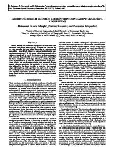
Fig. 1. A flowchart for speech emotion primitives estimation.

The present paper introduces several further new approaches on speech emotion estimation in 3D space, based on the VAM corpus. The overall flowchart is shown in Fig. 1. The main contributions are: 1. Three elementary estimators, i.e., robust regression, support vector regression, and locally linear reconstruction, for speech emotion estimation are introduced. They are diverse and complementary, in the sense that they cover both linear and nonlinear models, and both global and local models. All of them have comparable performance with the best estimator on the same dataset [14]. Among them, locally linear reconstruction (Section 3.4) is fairly new and has not been applied to emotion estimation. 2. We show that better performance can be obtained by properly fusing several elementary estimators. Two estimator fusion approaches, i.e., average fusion and locally weighted fusion, are introduced. Both of them outperform the elementary estimators, and also the best estimator on the same dataset [14]. Among them, locally weighted fusion (Section 4.2) is fairly new and has not been applied to emotion estimation. The rest of this paper is organized as follows: Section 2 introduces the data preparation procedure. Section 3 describes three elementary estimators. Section 4 introduces two estimator fusion approaches. Section 5 presents our experimental results. Finally, Section 6 draws conclusions and proposes future works. 2. DATA PREPARATION This section describes the sub-blocks in the “Data Preparation” block of Fig. 1 in detail.

using only five discrete numbers, after aggregation the final evaluations were almost continuous2 in [-1, 1]. The standard deviation of the evaluations for each utterance was also computed to measure the assessment quality. The mean standard deviation and mean correlation between the evaluators are listed in Table 1. Observe that the mean correlation of listeners’ evaluations on valence is much lower than those on activation and dominance. The mean correlation of listeners’ evaluations on valence is much lower than those on activation and dominance. An ANOVA test shows that the difference is statistically significant (F (2, 2838) = 42.82, p = 0). This suggests that for human listeners valence is more difficult to evaluate than activation and dominance; so, we expect that valence will also be more difficult to estimate. Table 1. Mean standard deviation and mean correlation of evaluations [14]. Mean standard deviation Mean Correlation V A D V A D 0.29 0.34 0.31 0.49 0.72 0.61 Previous research also supports the hypothesis that valence will be more difficult to estimate than either activation or dominance using audio information alone. In [20], the author states that the vocal channel alone is not sufficient for the estimation of valence. To fully capture the valence properties of an utterance, additional channels, such as video, are necessary. Contrastingly, activation is accurately conveyed using the audio information alone. In [17], the authors demonstrated, on a different dataset, that activation and dominance are highly correlated. It is therefore expected that dominance should also be accurately conveyed by the vocal channel. This hypothesis is supported by results demonstrated in [15].

2.1. Data Acquisition The database used in this study is the VAM Corpus, which contains spontaneous speech with authentic emotions recorded from guests in a German TV talk-show Vera am Mittag (Vera at Noon in English). The corpus was released in ICME2008 [16] and has been used by them in [12–15]. The database contains 947 emotional utterances from 47 speakers (11m/36f). All signals were recorded using a sampling frequency of 16 kHz and 16 bit resolution. 2.2. Emotion Primitives Evaluation A listener test was used to evaluate the emotion primitives in each utterance [12]. A group of evaluators listened to the emotional sentences and assessed the emotion primitives using the 5-point self assessment manikins (SAMs) [24]. One half of the database was evaluated by 17 listeners, the other by six, because the second half was evaluated later when a smaller number of evaluators was available. Intuitively, different listeners gave different evaluations for the same utterance. Grimm and Kroschel [12] merged them by a weighted average. Although each evaluator evaluated each sentence

2.3. Speech Feature Extraction Many different features can be extracted from speech signals, e.g., Lee and Narayanan [25] used a combination of acoustic, lexical, and discourse features to detect emotions in spoken dialogs. Among them, acoustic features [5,28] are most frequently used because they can be computed easily from speech signal. Major categories of acoustic features include fundamental frequency f0 (pitch), speaking rate, energy, spectral information, etc. However, it is still unclear which features are best suitable for emotion classification and estimation, and under what conditions. M = 46 acoustic features were used in our study. They are the same as those used by Grimm et al. [15] on the same corpus and cover four major categories: • Pitch related features (9): f0 mean, standard deviation, median, minimum, maximum, range, 25% and 75% quantiles, 2 True continuous annotations can be obtained by using the FEELTRACE tool [4]; however, currently it only supports annotations in the 2D activationevaluation space.

and the inter-quantile distance. • Speaking rate related features (5): mean and standard deviation of the duration of voiced segments, mean and standard deviation of the duration of unvoiced segments, ratio between the duration of unvoiced and voiced segments. • Energy related features (6): energy mean, standard deviation, maximum, 25% and 75% quantiles, and the inter-quantile distance. • Spectral features (26): mean and standard deviation of 13 Mel frequency cepstral coefficients (MFCC) [5]. We normalized each of the 46 features to the interval [0, 1] and then used them in all estimators introduced in the next section. Grimm and Kroschel [14] have also used 137 acoustic features, including the 46 features introduced above. Since the computational cost increases with the number of features, we only use the 46 features in this paper. Our goal is to demonstrate that estimator fusion can achieve better performance than a single estimator using a larger number of features. However, it is also interesting to study the performance of estimator fusion using more comprehensive features, which will be considered in our future research. 3. ELEMENTARY ESTIMATORS This section introduces three elementary estimators shown in the block “Elementary Estimators Construction” in Fig. 1, which have very diverse characteristics: 1. Robust regression (RR), which uses all training examples to construct a global linear regression model. 2. Support vector regression (SVR), which selects only a subset of the training examples (called support vectors) to construct a global nonlinear regression model. 3. Local linear reconstruction (LLR), which uses only nearest neighbors to construct a local linear regression model. In summary, our three elementary models cover both global models and local models, and both linear models and nonlinear models. So, they are diverse and complementary. Next, the procedure for feature ranking and selection for the three estimators is introduced before introducing the details of the three models.

RR [2, 3, 35] has shown to be more suitable for handling outliers and heteroscedasticity. The most frequently used RR method is Mestimation [21], and it was used in our study. Given a set of training examples {(xn , yn )}n=1,...,N , where xn ∈ RM , RR tries to fit a linear model M ∑

yn = a0 +

am xn,m + en

(1)

m=1

by minimizing the weighted objective function J=

N ∑

w(en )2 e2n

(2)

n=1

where en (n = 1, ..., N ) are the residuals, and a0 and am (m = 1, ..., M ) are the coefficients to be determined. Observe that the weight w(en ) is a function of the residual en . When w(en ) is a constant, the RR model reduces to the ordinary least squares model. In RR generally we require that w(en ) is a monotonically nonincreasing function of |en |, i.e., possible outliers get lower weights so that they do not affect the model too much. In the bisquare RR method [3, 9], the weight function is defined as { [1 − ( etn )2 ]2 , |en | ≤ t w(en ) = (3) 0, |en | > t where t is called a turning constant. Smaller values of t produce more resistance to outliers, but at the expense of lower efficiency when the errors are normally distributed [9]. t = 4.685, the default value in Matlab function robustfit, was used in our study. 3.3. Support Vector Regression (SVR) Support vector machine [38] is a very powerful tool for classification and estimation. In this paper it is used for regression and is called SVR. ϵ-SVR [39] was used by Grimm and Kroschel in [14] and achieved good performance. It was also implemented in this paper for comparison purpose. The procedure was the same as that in [14], except that 46 instead of 137 features were used. Due to space limit, interested readers should refer to [14] for further details. 3.4. Locally Linear Reconstruction (LLR)

3.1. Feature Ranking and Selection It is necessary to select a subset of the best features from the 46 features, because redundant features may deteriorate the estimation performance and also increase the computational cost. The wrapper method [19] was used in feature selection. We first rank the features using sequential backward selection [11], and then perform 10-fold cross-validation according to the rank of the features to select the best subset. 3.2. Robust Regression (RR) Intuitively, least squares regression can be used to estimate the emotion primitives from the 46 features; however, ordinary least squares estimation is not suitable for our problem because: 1. There may be outliers in the 947 utterances. In this case, ordinary least squares estimation is inefficient and can be biased. 2. Ordinary least squares estimation assumes a homoscedastic model, i.e., the standard deviation of the estimation error is a constant and does not depend on the inputs. Clearly, our dataset is heteroscedastic [1, 35] because different values of primitives have different standard deviations.

Grimm and Kroschel [14] constructed a k-nearest neighbor (k-NN) estimator for emotion primitive estimation and observed comparable performance with SVR. A variant of their approach is introduced in this section. Given a set of training examples {(xn , yn )}n=1,...,N and a new input x, the k-NN method first finds the k NNs of x according to a distance function. Denote the index set of these k NNs as Ix . Then, the output of the k-NN estimator is computed as: / ∑ ∑ yˆ = wi y i wi (4) i∈Ix

i∈Ix

The performance of k-NN estimator is determined by the number of NNs k, the distance function, and the weights wi . The k-NN estimator constructed by Grimm and Kroschel [14] used equal weights for the k NNs, which is the simplest approach. LLR, a variant of k-NN proposed by Kang et al. [22], is investigated in this paper because it assigns different weights to the NNs by considering the local topology. Moreover, Gupta and Mortensen [18] have shown that LLR minimizes bias and/or first-order error when it is used in weighted k-NN classification.

T LLR determines the weights w = (w1 , ..., ∑wk ) by minimiz1 ing the reconstruction error E(w) = 2 ||x − i∈Ix wi xi ||2 . This minimization problem can be solved explicitly, and the optimal w is:

w = (XT X)−1 XT x

(5)

where X is a matrix whose ith column is x∑ i . To eliminate estimation bias, we also need to normalize w so that i∈Ix wi = 1. 4. ESTIMATOR FUSION Multiple estimators fusion, a branch of the ensemble approach [27, 30], is an important research topic in signal processing and machine learning, because a fused model may have better performance than each elementary model. To guarantee performance improvement, we need multiple diverse elementary models and a good fusion strategy. In the previous section we have constructed three very diverse and complementary elementary estimators (i.e., linear/nonlinear models, and global/local models), and hence better performance is expected if they are fused properly. Next we will introduce two methods to fuse the three estimators, as shown in the “Estimator Fusion” block in Fig. 1. 4.1. Average Fusion (AF) Average fusion (AF) is the simplest model fusion method, where the fused output is simply the average output of the elementary estimators. Let yˆp (p = 1, ..., P ) be the output of the pth estimator. Then, the output of AF is yˆAF =

P 1 ∑ yˆp P p=1

(6)

4.2. Locally Weighted Fusion (LWF) AF weights the elementary estimators equally, whereas it may be more appropriate to assign different weights to different models because they have different accuracy, and utilize different aspects of the input data. Moreover, the local performance of a given model is usually not consistent over the entire input domain. So, it is possible to selectively leverage an elementary model’s locally superior accuracy to improve overall performance. This is the motivation of locally weighted fusion (LWF) [43]. Given a set of training examples {(xn , yn )}n=1,...,N , a new input x, and a group of P estimators, the procedure for LWF is: 1. Individual estimate calculation, where the outputs of the elementary estimators for x are computed. Denote them as yˆp , p = 1, ..., P . 2. Estimator local performance evaluation, where the weights {wp }p=1,...,P for the P elementary estimators are determined. There are different methods for local performance evaluation. A k-NN approach was used in this paper. First, k NNs of x are identified from the training examples, where the best features from LLR were used. Denote the index set of these k NNs as Ix . Then, each estimator is separately used to estimate the outputs for these k NNs. Denote Estimator p’s estimate for the ith NN as yˆp,i . Since the true outputs for these k NNs are known, the estimation error for each elementary estimator can be computed. The weight for the pth estimator is then computed as / ∑ wp = 1 |yi − yˆp,i | (7) i∈Ix

3. Estimator fusion, where the elementary estimates are fused as ∑P ˆp p=1 wp y yˆLW F = ∑P (8) w p p=1 5. EXPERIMENTAL RESULTS Our experimental results on the VAM dataset are reported in this section. To be consistent with the results in [14, 15], two measures are used in performance evaluation: • The mean absolute error (MAE) between the estimates, yˆn , and the human evaluations (references), yn . • The correlation coefficient (CC) between yˆn and yn . 5.1. Elementary Estimator Performance The performances of the three estimators were compared using 10fold cross-validation. The results are show in the first part of Table 2. The third part of Table 2 also shows the performance of a fuzzy logic system (FLS) [14,15] for emotion primitives estimation based on the same dataset, and the performance of the best estimator (SVR-RBF) reported in [14], which represents the state-of-the-art results on the VAM dataset. A graphic comparison of the performances is shown in Fig. 2. Observe that: 1. Each of our three elementary estimators outperformed FLS significantly. 2. Each of our three elementary estimators had comparable performance with SVR-RBF, the best estimator so far in the literature on the VAM dataset. Note that our estimators used only 1/3 of the features in SVR-RBF. So, this suggests that all of our three methods are very suitable for speech emotion estimation. 3. The correlation coefficient for valence is much lower than those for activation and dominance, which indicates it is more difficult to estimate valence. This is consistent with the case for human evaluators, as shown in Table 1, and in previous research [15, 20]. Table 2. Performance comparison of different estimators. Mean Absolute Error Correlation Estimator V A D V A D RR .1304 .1608 .1437 .4542 .8046 .7893 SVR .1334 .1542 .1438 .4460 .8241 .7871 LLR .1317 .1543 .1468 .5009 .8043 .7798 AF .1240 .1448 .1355 .5376 .8416 .8152 LWF .1225 .1409 .1342 .5456 .8472 .8185 FLS [14] .27 .17 .18 .28 .75 .72 SVR-RBF [14] .13 .15 .14 .46 .82 .79

5.2. Fusion Performance 10-fold cross-validation was also used in selecting the optimal k (number of NNs) for LWF. Remarkably, a very small number of NNs (2∼3 in our case) was enough to determine the local weights for LWF. The performance of AF and LWF are summarized in the second part of Table 2, and a graphic comparison with other estimators is shown in Fig. 2. Observe that though each of our three elementary estimators had similar performance as SVR-RBF, both of our fused models outperformed SVR-RBF, i.e., AF and LWF are effective estimator fusion strategies to boost performance. Especially, LWF achieved the best performance of all models.

FLS RR LLR SVR SVR−RBF AF LWF

0.24 0.22 0.2 0.18 0.16 0.14

Valence

Activation

(a)

Dominance

Correlation Coefficient (CC)

Mean Absolute Error (MAE)

0.26

0.8 0.7

LWF AF LLR SVR−RBF RR SVR FLS

0.6 0.5 0.4 0.3

Valence

Activation

Dominance

(b)

Fig. 2. Performance comparison of the five estimators proposed in this paper and two methods in [14]. (a) MAE; and, (b) CC. The black curve in each sub-figure represents the best performance in the literature on the VAM dataset. The dashed curves are our elementary models. For (a), a lower curve represents a better performance. For (b), a higher curve represents a better performance.

The percentage of performance improvement of LWF over the other six models are shown in Table 3. Observe that for MAE, LWF was able to gain 6.02-12.40% improvement over each elementary model, and for CC, the performance improvement was 2.80-22.35%. Additionally, LWF had 0.95-2.68% performance improvement over AF on MAE, which was due to the utilization of local performance information. Table 3. Percentage of performance improvement of LWF over the other six approaches. Mean Absolute Error Correlation Estimator V A D V A D RR 6.02 12.40 6.64 20.13 5.29 3.70 8.13 8.65 6.66 22.35 2.80 3.99 SVR LLR 6.98 8.71 8.61 8.93 5.33 4.97 AF 1.18 2.68 0.95 1.49 0.66 0.41 FLS [14] 54.62 17.12 25.45 94.86 12.96 13.69 SVR-RBF [14] 5.75 6.07 4.15 18.61 3.32 3.61 To see whether the performances of the elementary estimators and the fusion models are significantly different, we also performed ANOVA tests on the MAEs. The results are shown in Table 4. Observe that generally the differences in MAE between the elementary estimators and the fusion models are statistically significant.

Table 4. p-values of ANOVA tests on the MAEs between the elementary estimators and the two fusion models. AF LWF Estimator V A D V A D RR .24 .15 0 0 .12 .07 SVR .08 .04 .08 .01 .12 .07 .14 .08 .10 .02 .03 .02 LLR

6. CONCLUSIONS AND FUTURE WORKS Speech information processing is very important for affective computing. Most research in this direction has focused on classifying emotions into a small number of categories. However, numerical representations of emotions in a multi-dimensional space can be more convenient for human-computer interaction because computers are better at processing numbers, and also sometimes we

only need to deal with a subset of the emotion primitives. Several approaches for emotion primitives estimation in 3D space (valence/activation/dominance) have been presented in this paper. They were compared with the state-of-the-art results on the same dataset. The main findings are: 1. Robust regression, support vector regression, and locally linear reconstruction are very suitable for speech emotion estimation. All of them have comparable performance with the best estimator on the same dataset. 2. Better performance can be obtained by properly fusing several elementary estimators. Particularly, locally weighted fusion, which weights each elementary estimator by its local performance around the new input, appears promising. Our future research includes: 1. Using more features to improve estimation accuracy. Extra features can be considered, e.g., Grimm and Kroschel [14] extracted 137 acoustic features (three times as many as ours) from the same corpus, and Lee and Narayanan [25] considered lexical and discourse features in addition to acoustic features. Additionally, Lu et al. [26] reported that Mel-Frequency Filter Banks (MFBs) are better features than MFCCs in text-independent speaker identification. Since MFCCs were the most important features in our study, it is interesting to investigate how MFBs are useful in speech emotion estimation. 2. Filtering the estimates using the knowledge that usually emotion changes slowly. It is very rare in real life that a person’s emotion changes rapidly from one utterance to the next. So, a filter can be designed to smooth the estimates. 3. Applying our algorithms to emotion estimation from physiological signals or facial expressions. As long as features from physiological signals or facial expressions are extracted, our algorithms can be applied directly. 7. REFERENCES [1] T. S. Breusch and A. R. Pagan, “A simple test for heteroscedasticity and random coefficient variation,” Econometrica, vol. 47, no. 5, pp. 1287–1294, 1979. [2] R. J. Carroll and D. Ruppert, “Robust estimation in heteroscedastic linear models,” The Annals of Statistics, vol. 10, no. 2, pp. 429–441, 1982. [3] W. S. Cleveland, “Robust locally weighted regression and smoothing scatterplots,” Journal of the American Statistical Association, vol. 74, pp. 829–836, 1979. [4] R. Cowie, E. Douglas-Cowie, S. Savvidou, E. Mcmahon, M. Sawey, and M. Schr¨oder, “FEELTRACE: An instrument for recording perceived emotion in real time,” in Proc. ISCA Workshop on Speech and Emotion, Northern Ireland, UK, September 2000, pp. 19–24. [5] S. Davis and P. Mermelstein, “Comparison of parametric representations for monosyllabic word recognition in continuously spoken sentences,” IEEE Trans. on Acoustics, Speech and Signal Processing, vol. 28, no. 4, pp. 357–366, 1980. [6] E. Douglas-Cowie, R. Cowie, and M. Schr¨oder, “A new emotion database: Considerations, sources and scope,” in Proc. ISCA ITRW on Speech and Emotion, Newcastle, UK, September 2000, pp. 39–44. [7] S. H. Fairclough, “Fundamentals of physiological computing,” Interacting with Computers, vol. 21, pp. 133–145, 2009.

[8] B. Fasel and J. Luettin, “Automatic facial expression analysis: a survey,” Pattern Recognition, vol. 36, no. 1, pp. 259–275, 2003. [9] J. Fox, “Robust regression,” 2002. [Online]. Available: http://cran.r-project.org/doc/contrib/Fox-Companion/ appendix-robust-regression.pdf. [10] N. F. Fragopanagos and J. G. Taylor, “Emotion recognition in human-computer interaction,” Neural Networks, vol. 18, no. 4, pp. 389–405, 2005. [11] K. S. Fu, Sequential Methods in Pattern Recognition and Machine Learning. NY: Academic Press, 1968. [12] M. Grimm and K. Kroschel, “Evaluation of natural emotions using self assessment manikins,” in Proc. IEEE Automatic Speech Recognition and Understanding Workshop, San Juan, Pueto Rico, November 2005, pp. 381–385. [13] ——, “Rule-based emotion classification using acoustic features,” in Proc. 3rd Int’l Conf. on Telemedicine and Multimedia, Kajetany, Poland, October 2005. [14] ——, “Emotion estimation in speech using a 3D emotion space concept,” in Robust Speech Recognition and Understanding, M. Grimm and K. Kroschel, Eds. Vienna, Austria: I-Tech, 2007, pp. 281–300. [15] M. Grimm, K. Kroschel, E. Mower, and S. Narayanan, “Primitives-based evaluation and estimation of emotions in speech,” Speech Communication, vol. 49, pp. 787–800, 2007. [16] M. Grimm, K. Kroschel, and S. Narayanan, “The Vera Am Mittag German audio-visual emotional speech database,” in Proc. Int’l Conf. on Multimedia and Expo, Hannover, German, June 2008, pp. 865–868. [17] M. Grimm, E. Mower, K. Kroschel, and S. S. Narayanan, “Combining categorical and primitives-based emotion recognition,” in Proc. European Signal Processing Conf., Florence, Italy, September 2006. [18] M. R. Gupta and W. Mortensen, “Weighted nearest neighbor classifiers and first-order error,” in Proc. Intl. Conf. on Frontiers of Interface Between Statistics and Science, Hyderabad, Andra Pradesh, India, December 2009. [19] I. Guyon and A. Ellisseeff, “An introduction to variable and feature selection,” Journal of Machine Learning Research, vol. 3, p. 2003, 1157-1182. [20] A. Hanjalic, “Extracting moods from pictures and sounds: Towards truly personalized TV,” IEEE Signal Processing Magazine, vol. 23, no. 2, pp. 90–100, March 2006. [21] P. J. Huber, “Robust estimation of a location parameter,” Annals of Mathematical Statistics, vol. 35, pp. 73–101, 1964. [22] P. Kang and S. Cho, “Locally linear reconstruction for instance-based learning,” Pattern Recognition, vol. 41, pp. 3507–3518, 2008. [23] R. Kehrein, “The prosody of authentic emotions,” in Proc. Speech Prosody Conf., Aix-en-Provence, France, April 2002, pp. 423–426. [24] P. J. Lang, “Behavioral treatment and bio-behavioral assessment,” in Technology in Mental Health Care Delivery Systems, J. B. Sidowski, J. H. Johnson, and T. A. Williams, Eds. Norwood, NJ: Ablex Publishing, 1980, pp. 119–137. [25] C. M. Lee and S. Narayanan, “Toward detecting emotions in spoken dialogs,” IEEE Trans. on Speech and Audio Processing, vol. 13, no. 2, pp. 293–303, 2005.

[26] H. Lu, H. Okamoto, M. Nishida, Y. Horiuchi, and S. Kuroiwa, “Text-independent speaker identification based on feature transformation to phoneme-independent subspace,” in Proc. IEEE Int’l Conf. on Communication Technology, Hangzhou, China, November 2008, pp. 692–695. [27] D. Opitz and R. Maclin, “Popular ensemble methods: An empirical study,” Journal of Artificial Intelligence Research, vol. 11, pp. 169–198, 1999. [28] P.-Y. Oudeyer, “The production and recognition of emotions in speech: features and algorithms,” International Journal of Human-Computer Studies, vol. 59, pp. 157–183, 2003. [29] R. Picard, Affective Computing. Cambridge, MA: The MIT Press, 1997. [30] R. Polikar, “Ensemble based systems in decision making,” IEEE Circuits and Systems Magazine, vol. 6, pp. 21–45, 2006. [31] J. A. Russell, “Core affect and the psychological construction of emotion,” Psychological Review, vol. 110, pp. 145–172, 2003. [32] H. Schlosberg, “Three dimensions of emotion,” Psychological Review, vol. 61, no. 2, pp. 81–88, 1954. [33] M. Schr¨oder, R. Cowie, E. Douglas-Cowie, M. Westerdijk, and S. Gielen, “Acoustic correlates of emotion dimensions in view of speech synthesis,” in Proc. Eurospeech, Aalborg, Denmark, September 2001, pp. 87–90. [34] B. Schuller, M. Lang, and G. Rigoll, “Recognition of spontaneous emotions by speech within automotive environment,” in Proc. German Annual Conf. on Acoustics, Braunschweig, Germany, March 2006, pp. 57–58. [35] A. H. Studenmund, Using Econometrics: A Practical Guide, 5th ed. Addison Wesley, 2005. [36] A. Tan and R. Muhlberger, “From operator to interaction: Designing an affective computing system for interactive lighting,” in Proc. Computer/Human Interaction Conf., Boston, MA, April 2009. [37] J. Tao and T. Tan, “Affective computing: A review,” Lecture Notes in Computer Science, vol. 3784, pp. 981–995, 2005. [38] V. Vapnik, The Nature of Statistical Learning Theory. Berlin: Springer-Verlag, 1995. [39] ——, Statistical Learning Theory. New York, NY: Wiley, 1998. [40] L. Vidrascu and L. Devillers, “Real-life emotion representation and detection in call center data,” in Proc. Int’l Conf. on Affective Computing and Intelligent Interaction, Beijing, China, October 2005, pp. 739–746. [41] M. W¨ollmer, F. Eyben, S. Reiter, B. Schuller, C. Cox, E. Douglas-Cowie, and R. Cowie, “Abandoning emotion classes - towards continuous emotion recognition with modelling of long-range dependencies,” in Proc. 9th Annual Conf. of the Int’l Speech Communication Association (InterSpeech), Brisbane, Australia, September 2008, pp. 597–600. [42] W. Wundt, Grundriss der Psychologie. Leipzig: W. Engelmann, 1896. [43] F. Xue, R. Subbu, and P. Bonissone, “Locally weighted fusion of multiple predictive methods,” in Proc. IEEE Int’l Joint Conf. on Neural Networks, Vancouver, BC, Canada, July 2006, pp. 2137–2143. [44] C. Yu, P. Aoki, and A. Woodruff, “Detecting user engagement in everyday conversations,” in Proc. Int’l Conf. on Spoken Language Processing, Jeju Island, Korea, October 2004, pp. 1329– 1332.