Term Structure of Consumption Risk Premia in the Cross Section of Currency Returns Journal of Finance, forthcoming

Irina Zviadadze

∗

July 4, 2016 Abstract

I relate the downward sloping term structure of currency carry returns to compensations for currency exposures to macroeconomic risk embedded in the joint dynamics of US consumption, inflation, nominal interest rate, and their stochastic variance. The interest rate and inflation shocks play a prominent role. Higher yield currencies exhibit higher multi-period exposures to these shocks. The prices of these risk exposures are positive and sizeable across all investment horizons. The interest rate shock operates qualitatively similar to the long-run risk of Bansal and Yaron (2004). ∗

Zviadadze is at the Stockholm School of Economics. I am grateful to the Editor, Kenneth Singleton, the anonymous Associate Editor and two Referees for the constructive feedback. I am indebted to my advisors, Mikhail Chernov and Francisco Gomes, for their unconditional support, stimulating discussions and helpful suggestions. I am also very grateful to David Backus, Jaroslav Boroviˇcka, Tomas Bjork, Laurent Calvet, Joao Cocco, Riccardo Colacito, Mariano M. Croce, Magnus Dahlquist, Vito Gala, Jeremy Graveline, David Edgerton, Lars Hansen, Christian Heyerdahl-Larsen, Christian Julliard, Leonid Kogan, Lars Lochstoer, Igor Makarov, Michael Moore, Ivan Shaliastovich, Paolo Surico, Stijn Van Nieuwerburgh, Christian Wagner, and Stanley Zin for advice and detailed feedback. I also thank many participants of conferences and seminars, including Early Career Women in Finance, Frontiers of Finance Warwick, SED, SoFiE, Young Scholars Nordic Finance Workshop, WFA, World Congress of Econometric Society, Bocconi, HEC Paris, LBS, LSE, Lund University, New Economic School, Rutgers Business School, Stockholm School of Economics, Sveriges Riksbank, UNC Kenan-Flagler Business School, and UCLA Anderson School of Management for many helpful discussions and comments. I gratefully acknowledge the financial support from the AXA research fund, Jan Wallander and Tom Hedelius Foundation, and the Swedish House of Finance. The author has no conflicts of interest, as identified in the Disclosure Policy.

I quantify the risk-return relationship in the foreign exchange (FX) market across different countries and investment horizons. My starting point is new evidence about returns on a currency carry trade, a zero-cost investment strategy of buying bonds in high yield currencies and short selling bonds in low yield currencies, across alternative investment horizons. The term structure of average carry log returns is slightly downward sloping: the average log returns are 1.13% and 0.80% per quarter at the three-month and ten-year investment horizons, respectively. I ask which sources of macroeconomic risk are compensated in the term structure of carry returns. Shocks to consumption growth, inflation, interest rates, and their second order moments reflect different aspects of currency risk. My focus is on the identification of such shocks, measuring their impact on exchange rates in the cross section and at alternative horizons, and understanding their relative importance for carry trade profitability across alternative investment horizons. I find that the interest rate and inflation shocks play a prominent role. Higher yield currencies exhibit higher multi-period exposures to these shocks. The prices of these risk exposures are positive and sizeable across all investment horizons. The interest rate shock contributes most to the cross sectional differences in currency returns across multiple investment horizons and operates qualitatively similar to the long-run risk of Bansal and Yaron (2004). My analysis proceeds in two stages. At the first stage, I describe the empirical properties of currency risk related to macroeconomic fluctuations. To this end, I estimate the joint dynamics of US consumption growth, inflation, nominal interest rate, and the cross section of exchange-rate growths as a vector autoregression (VAR) with stochastic variance. I compute shock-exposure elasticities (Boroviˇcka and Hansen, 2014; Boroviˇcka, Hansen, Hendricks, and

1

Scheinkman, 2011; Zviadadze, 2015) of exchange rates to measure importance of macroeconomic shocks identified from the VAR. Shock-exposure elasticities are marginal multi-period risk sensitivities of exchange rates to alternative current period shocks. Intuitively, a source of risk is economically interesting if the shock-exposure elasticities of low and high interest rate currencies exhibit high dispersion at alternative horizons. I document economically sizeable and statistically significant gaps between the shockexposure elasticities in the cross section of currency baskets. Higher yield currencies exhibit higher exposures to the interest rate and inflation shocks across multiple investment horizons. To the best of my knowledge, this is the first study that explicitly relates the interest rate and inflation shocks, identified from the US macroeconomic data, to the cross section of currency baskets, and explores the term structure of currency exposures to macroeconomic risk. Thus, these novel facts complement the influential evidence of Lustig and Verdelhan (2007) in a nontrivial way. The dispersion in multi-period currency exposures to the sources of risk is a necessary but not sufficient condition for relating the cross sectional spread in currency returns across alternative investment horizons to the macroeconomic risk. An outstanding question is whether the currency risk sensitivity has an economically sizeable price. This is where the second stage of my analysis comes in. In order to measure price of risk, I introduce a US representative agent with recursive utility and an aversion to consumption risk and interpret the estimated VAR as a model of consumption growth with the explicitly specified dynamics of the expected consumption growth and stochastic variance. Consequently, the macroeconomic shocks represent multiple sources of consumption risk. Combining the VAR with recursive preferences comes with its challenges. The nominal 2

yield plays a dual role. On the one hand, the pricing kernel depends on the nominal yield, as it is one of the state variables in the model. On the other hand, the nominal yield is the (log) conditional expectation of the pricing kernel and, therefore, an affine function of the model’s states. The first-order condition implies a set of pricing restrictions on the structural parameters of the model. These structural restrictions imposed on the parameters of the VAR lead to nontrivial complications in estimation that I resolve by using Bayesian MCMC. Armed with the estimated dynamics of the pricing kernel, I characterize how currency sensitivities to macroeconomic risk are compensated in the marketplace at horizons from one quarter up to ten years. Shock-price elasticities (Boroviˇcka and Hansen, 2014; Boroviˇcka, Hansen, Hendricks, and Scheinkman, 2011; Zviadadze, 2015) assign prices to shock-exposure elasticities. Put simply, shock-price elasticities constitute a term structure of marginal prices of risk, or term structure of marginal Sharpe ratios. The analysis of the shock elasticities reveal that the interest rate risk plays the most prominent role in the foreign exchange market. There are two important properties that lead to this conclusion. First, I confirm in the context of the structural VAR that higher yield currencies exhibit larger sensitivities to the shock at horizons from one quarter up to sixteen quarters.1 This fact means that upon realization of the positive shock, high yield currencies are expected to appreciate relative to low yield currencies during a four-year time period. Second, the marginal price for bearing interest rate risk is the largest at all investment horizons. Taken together, the term structure of currency risk premia reflects the interest rate shock at short- and medium-term horizons. An examination of the empirical properties of the interest rate shock suggests that this risk operates qualitatively similar to the long-run risk of Bansal and Yaron (2004). First, the 3

shock affects consumption growth only with a lag of one quarter. Second, the shock originates via a persistent variable and has the highest price of risk. Finally, it is the dominant source of variation in the real risk-free rate. These empirical results complement the argument of Colacito and Croce (2013) about the special role of the long-run risk in currency markets. Their conclusion is based on a symmetric two-country setting which, by construction, does not accommodate the term structure of the cross sectional spreads in currency risk premia. I leave the question of identifying the economic origins of the long-run risk shock operating in the foreign exchange market for future research. Estimation of the structural VAR reveals that, similarly to the interest rate shock case, higher yield currencies have higher exposures to the inflation shock across multiple investment horizons. The marginal price of the shock is less sizeable than that of the interest rate shock but it is economically meaningful. Given the quantitative prominence of the inflation shock in the term structure of currency carry premia, future models of foreign exchange risk should explore not only real, as it has been mostly done so far, but also nominal sources of risk. The variance shock contributes to the term structure of currency risk premia in a conceptually different way. Currencies are not sensitive to the variance shock at any investment horizon, yet it is the only source of time variation in the risk premium. As a result, the log expected return on the one-period carry trade strategy, for example, has fluctuated historically between 0.43% and 3.54% per quarter. The role of the consumption growth shock is limited to high yield currencies at the oneperiod investment horizon. The average price for bearing a three-month exposure of high yield currencies to the consumption growth shock is about 0.24% per quarter. Thanks to the 4

high compensation of the one-period exposure of high yield currencies to the consumption growth shock, the carry risk premium is largest at the three-month investment horizon. The cross section of currency risk premia as compensation for currency exposures to the macroeconomic risk exhibits a downward sloping term structure. At the short- and mediumterm end, the carry risk premia are rather flat and reaches the level of about 1.31% per quarter, on average. At horizons longer than ten quarters, the risk premia are statistically insignificant. Hence, the profitability of investments in bonds of high interest rate currencies, when the money is borrowed in low interest rate environments, is a short- to medium-horizon phenomenon. This paper is related to the international macro-finance literature that examines timeseries and cross sectional properties of currency risk premia. I limit my discussion to papers that interpret currency risk premia as compensation for macroeconomic risk. On the empirical side, Cumby (1988), Lustig and Verdelhan (2007), and Sarkissian (2003) study the ability of the consumption growth factor to explain the cross section of currency returns. The authors consider different cross sections of currency returns: Cumby (1988) and Sarkissian (2003) study individual currencies, whereas Lustig and Verdelhan (2007) examine interestrate-sorted currency portfolios. Cumby (1988) shows that the ex-ante currency returns and the conditional covariances between currency excess returns and US consumption growth connect in a way that is consistent with consumption-based models. Formal testing, however, reveals that basic models, for example, models with a time-separable utility function, cannot quantitatively account for the behavior of currency returns. Sarkissian (2003) adapts the framework of Constantinides and Duffie (1996) to a multi5

country setting and shows that the cross-country variance of consumption growth has explanatory power for cross sectional differences in returns on individual currencies, whereas the consumption growth itself does not. Lustig and Verdelhan (2007) use the framework of the durable CCAPM of Yogo (2006) to establish that the consumption growth is a priced factor in the cross section of returns on currency baskets formed by sorting currencies by respective interest rates. Sarkissian (2003) and Lustig and Verdelhan, 2007) have two common threads. First, both studies recognize the presence of multiple sources of consumption risk but do not describe them explicitly. Second, neither paper extends the analysis beyond a single horizon given by the decision interval of the representative agent (one quarter in the case of Sarkissian, 2003, and one year in the case of Lustig and Verdelhan, 2007). My study fills this void by linking profitability of interest-rate-sorted currency portfolios to multiple sources of consumption risk across alternative investment horizons. The theoretical literature features different macro-based models dedicated to rationalizing the time variation in currency log returns, for example, the violation of the uncovered interest rate parity (Fama (1984) regressions). The models include settings with habits (Heyerdahl-Larsen, 2014; Verdelhan, 2010), long-run risks (Bansal and Shaliastovich, 2013; Colacito, 2009; Colacito and Croce, 2013), and disasters (Farhi and Gabaix, 2016). This paper builds on important lessons drawn from the international long-run risk literature, yet it makes a number of complementary independent contributions. For example, an influential paper by Colacito and Croce (2011) suggests a link between international long-run risk and exchange rate movements. My empirical results reflect the importance of this economic mechanism from a novel perspective: I document the multi-period heterogenous risk ex-

6

posures of low and high yield currencies to the domestic interest rate shock that operates qualitatively similar to the long-run risk. The two-country symmetric theoretical model of Colacito and Croce (2011) does not imply the presence of such a cross section of currency risk exposures across alternative investment horizons (see expression (5) in their paper). My paper adds to a rapidly growing literature on the term structures of various assets. So far there has been no explicit study of the effect of the investment horizon on the profitability of carry trades. Recently Lustig, Stathopoulos, and Verdelhan (2016) have analyzed the profitability of investing in bonds of different maturities across the globe over one period. They document lower average returns on strategies involving longer-term bonds and rely on the assumption of market completeness to interpret this fact as a manifestation of the stationarity of exchange rates. Furthermore, they establish the connection between stationarity of exchange rates and the uncovered interest rate parity at an infinite investment horizon. I characterize the term structure of average carry log returns and explain its shape and level in a flexible consumption-based model of the representative agent with recursive preferences without relying on assumption of market completeness. My analysis is silent about the properties of the investment strategy considered by Lustig, Stathopoulos, and Verdelhan (2016), as I deliberately choose not to model the foreign pricing kernel. Thus, I see my study and paper by Lustig, Stathopoulos, and Verdelhan (2016) as complementary sources of evidence on multi-period profitability of investment strategies involving trades in bonds of different countries and different maturities. My analysis delivers empirical facts which future general equilibrium models of currency risk should be consistent with: the interest rate and inflation shocks are reflected in the term structure of carry returns; the interest rate shock plays the most prominent role in currency 7

pricing and operates qualitatively similar to the long-run risk of Bansal and Yaron (2004). In addition, my findings emphasize the presence of asymmetry across countries, highlighted earlier in Backus, Foresi, and Telmer (2001) and Lustig, Roussanov, and Verdelhan (2011) among others, and the prominence of not only real but also nominal risk in the foreign exchange market. Finally, my paper is related to Hansen, Heaton, and Li (2008), which provides evidence of the importance of the permanent shock to consumption in accounting for the value premium. Both papers use a similar methodology of modeling the pricing kernel (under the assumption of recursive preferences) jointly with asset cash flows. My study differs from Hansen, Heaton, and Li (2008) in three principal dimensions. First, I study the foreign exchange market, which has been examined to a lesser degree than the US equity market. Second, my model has stochastic variance: I account for the variation in the volatility of consumption growth and, therefore, in risk premia. Third, I quantify the relative importance of consumption shocks for short and medium horizons, rather than at an infinite horizon. The paper is organized as follows. Section I presents evidence on the term structure of average carry log returns and empirically analyzes in a reduced form how dynamics of the cross section of exchange rates relates to macroeconomic shocks. Section II develops an equilibrium framework for studying how the term structure of currency returns reflects multiple sources of consumption risk, and discusses the estimation methodology. Section III documents the estimation results: (i) term structure of consumption risk in the cross section of currency baskets, (ii) term structure of prices of consumption shocks in the cross section of currency baskets, (iii) term structure of consumption risk premia in the cross section of currency returns; and discusses the economic underpinnings of the foreign-exchange risk.

8

Section IV concludes. Four appendices contain description of the dataset, solution of the model, and estimation output. The online Appendix contains supplementary robustness checks and various methodological details.

1

Macroeconomic risk in the cross section of exchange rates

A

Multi-period profitability of carry trades I explore the term structure of average carry log returns with holding periods ranging

from one quarter to ten years. At the end of each quarter, the currencies of twelve large economies are sorted based on their interest rates and allocated to three equally weighted baskets: basket “Low” (low interest rate currencies), basket “Intermediate” (intermediate interest rate currencies), and basket “High” (high interest rate currencies). The cross-term foreign interest rate,

˜it =

T 1 X˜ it,t+τ , T τ =1

serves as a sorting variable where symbol T = 40 denotes the number of maturities in the foreign term structure and ˜it,t+τ stands for a foreign yield of maturity τ - periods (quarters) at time t.2 Because the average yield aggregates information from the entire yield curve, this sorting separates low and high interest rate currencies across different investment horizons. A unit investment horizon is one quarter. Table 1 shows the dynamic composition of currency Table 1 is about 9

here

baskets; Appendix A describes the sample and data sources. An investor follows a simple investment strategy. She borrows US dollars at the τ − period risk-free rate it,t+τ , converts the money into the foreign currencies of one of the baskets, buys τ − period foreign risk-free bonds, and at time t + τ converts the proceeds back into US dollars to pay off the debt. The log excess return for this strategy applied to an individual foreign currency is

log rxt,t+τ = log st+τ − log st + ˜it,t+τ − it,t+τ ,

where the exchange rate st is the nominal price of a foreign currency in US dollars. The log excess return for a currency basket is the equal-weighted average log excess return across all currencies in the basket. I use relationship between average log excess returns and yields highlighted by Backus, Boyarchenko, and Chernov (2015),

E(log rxt,t+τ − log rxt,t+1 ) = E(˜it,t+τ − ˜it,t+1 ) − E(it,t+τ − it,t+1 ),

to compute average carry log returns with holding periods longer than one quarter. First, I compute the common component of average log excess returns with alternative holding periods – the average log excess return for a one-period investment horizon E log rxt,t+1 . Then I add the corresponding difference in average yield slopes between the foreign and US nominal bonds, E(˜it,t+τ − ˜it,t+1 ) − E(it,t+τ − it,t+1 ), to the one-period average log excess return. Thus, I construct the entire term structure of average log returns on currency trade. The main advantage of this method, as explained in Backus, Boyarchenko, and Chernov 10

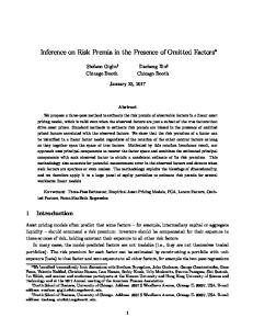
(2015), is the fact that computation of longer-horizon average log returns is not associated with a declining number of available non-overlapping data points. Figure 1 displays the spread in average currency log returns on “High” and “Low” currency baskets across alternative investment horizons. The term structure of carry log Figure 1 returns is slightly downward sloping. The average log return is 1.13% per quarter at the is about three-month investment horizon and 0.80% per quarter at the ten-year investment horizon. here This representation of average profitability of carry trades as a function of investment horizon is new and represents the central stylized fact of my study.3 It is customary in the literature to sort currencies based on their corresponding shortterm interest rates. This is so because the authors seek to understand the origins of the violation of the uncovered interest parity or carry profitability at short horizons. In the current sample, the short-term sorting generates a downward sloping term structure of average carry log returns with a somewhat steeper slope than that in the cross-term sorting. The average carry log return is 1.02% per quarter at the three-month horizon and 0.57% per quarter at the ten-year investment horizon. Below, I conduct my analysis for the cross section of currency baskets sorted by the cross-term foreign rates. The results are robust with respect to the choice of the sorting variable. Section A.1 of the online Appendix describes multi-period profitability of carry trades formed by sorting currencies by the short-term rates and presents the equilibrium analysis of the macroeconomic risk-currency return tradeoff.

11

B

Joint dynamics of macroeconomic fundamentals and exchange rates A joint model of macroeconomic fundamentals and the cross section of exchange rate

growths is informative about the interplay between the macroeconomic and currency risks. Motivated by the extant literature, I choose macroeconomic variables that serve as modeling ingredients in my quantitative analysis. As Lustig and Verdelhan (2007) document, the cross section of currency returns reflects the US consumption growth risk at the investment horizon matching the decision interval of the representative agent. Thus, the US consumption growth is the first variable under consideration. There are distinct shocks affecting the expected consumption growth and the variance of consumption growth. To measure those, I model consumption growth jointly with US inflation, three-month nominal yield, and their common stochastic variance factor as a vector autoregression with stochastic variance. The aforementioned variables are known to have forecasting power for future consumption growth. Hall (1978) and Hansen and Singleton (1983) show that lagged consumption growth is useful in predicting future US consumption growth. Piazzesi and Schneider (2006) argue that inflation is a leading recession indicator. Bansal, Kiku, and Yaron (2012), Colacito and Croce (2011), and Constantinides and Ghosh (2011) argue that the real risk-free rate serves as a direct measure of the predictable component in future consumption growth. Because data on real rates, such as inflation-indexed bonds, are available only from 1997, I use a short-term nominal rate and inflation. In addition, the presence of such variables as real consumption growth and inflation helps the model capture both real and nominal macroeconomic fluctuations. 12

Signals embedded in the nominal interest rates and stochastic variance prove important in currency markets. First, the extensive literature on the UIP violation interprets the violation as a direct manifestation of time variation in the FX risk premium, and relates interest rate risks to those in exchange rates (e.g., Bansal and Shaliastovich, 2013; HeyerdahlLarsen, 2014; Verdelhan, 2010). Second, empirical macroeconomic studies emphasize that exchange rates do respond to shocks affecting interest rates. For example, Eichenbaum and Evans (1995) and Faust and Rogers (2003) quantify the impact of monetary policy shocks, identified through the dynamics of interest rates, on exchange rates. Finally, the stochastic variance of macroeconomic variables, that is the silent feature of macroeconomic data (e.g., Bansal, Kiku, Shaliastovich, and Yaron, 2014; Campbell, Giglio, Polk, and Turley, 2015; Kandel and Stambaugh, 1990; Whitelaw, 2000), serves as the source of time variation in the currency risk premium. I posit that the dynamics of the macroeconomy is described by a discrete-time model with a state Xt = (log gt , log πt , it,t+1 , vt )0 , where log gt is log consumption growth, log πt is log inflation, it,t+1 is three-month nominal yield, and vt is a common stochastic variance factor. I group the first three variables into a vector Yt = (log gt , log πt , it,t+1 )0 which is assumed to follow the vector autoregressive process of order one:

Yt+1 =

1/2

F + G Yt + Gv vt + Hv (vt+1 − Et vt+1 ) + H vt εt+1 .

3×1

3×3

3×1

3×1

3×3

(1)

The factor vt+1 ∼ ARG(1) is assumed to follow a scalar autoregressive gamma process of order one with the scale parameter σv2 /2, the degrees of freedom 2(1 − ϕv )/σv2 , and the serial

13

correlation parameter ϕv : vt+1 = (1 − ϕv ) + ϕv vt + σv ((1 − ϕv + 2ϕv vt )/2)1/2 εvt+1 .

(2)

The autoregressive gamma process can be viewed as the discrete-time counterpart to the continuous-time square-root model. See, for example, Gourieroux and Jasiak (2006) and Le, Singleton, and Dai (2010). The attractive feature of the autoregressive gamma process is the affine functional form of its cumulant generating function, and hence the overall tractability of the model. The model has four structural shocks. Three are the components of the vector εt+1 = (εgt+1 , επt+1 , εit+1 )0 . The fourth shock εvt+1 is the shock to the stochastic variance vt+1 . The shocks εt+1 ∼ MN (0, I) follow the multivariate normal distribution, whereas the shock εvt+1 is, by definition of the autoregressive gamma processes, nonnormal. Henceforth, I refer to the discrete-time four-state model (1)-(2) as a VAR model with stochastic variance. This VAR can be viewed as the data-generating process for consumption growth with the explicitly specified dynamics of the expected consumption growth and stochastic variance. Consequently, the structural shocks εt+1 and εvt+1 represent multiple sources of consumption risk. Carriero, Clark, and Marcellino (2015) show that a reduced form vector autoregression with a common stochastic variance factor efficiently summarizes the informative content of several macroeconomic variables and asset prices, including consumption growth, GDP inflation, the 10-year Treasury bond yield, and the federal funds rate. Their results motivate my choice of a model with only one stochastic variance factor as a compromise between good fit and parsimony. 14

The dynamics of three currency baskets complement the macroeconomic model (1)-(2). I posit that the log exchange-rate growth of each currency basket, log δt,t+1 = log st+1 −log st , loads on the macroeconomic states and shocks as follows: 1/2

log δt,t+1 = log δ + µ0 Yt + µv vt + ξ 0 vt εt+1 1/2 + ξv [(1 − ϕv + 2ϕv vt )/(1 + ϕv )]1/2 εvt+1 + ξ˜w vt w˜t+1 .

(3)

The elements of the vectors µ and ξ, as well as the parameters µv and ξv reflect the impact of both US and foreign macroeconomic fundamentals on currency dynamics, as long as the foreign variables are not orthogonal to the states Xt = (Yt0 , vt )0 and shocks εt+1 and εvt+1 .4 1/2 The process (3) has a component ξ˜w vt w˜t+1 aggregating the impact of idiosyncratic (foreign

specific, orthogonal to the shocks εt+1 and εvt+1 ) disturbances on the exchange-rate growth, but omits a vector of foreign-specific (orthogonal to Xt ) states. The absence of foreignspecific states does not impede the unbiased measurement of the parameters µ, ξ, µv , and ξv . The online Appendix (Section A.2) provides details. I use Bayesian MCMC methods to estimate the vector autoregression (1)–(3) on a sample of quarterly US macroeconomic data from 1947 to 2011 and quarterly currency data from 1986 to 2011. Table 2 provides basic descriptive statistics. The Bayesian approach has Table 2 a number of important advantages. First, it delivers the estimated time-series of stochastic is about variance vt as a byproduct of the estimation routine. Second, it accounts for parameter and here state uncertainty (vt ), thereby facilitating estimation, as it can be implemented in two stages similar to that of Hansen, Heaton, and Li (2008). At the first stage, I estimate the dynamics of macroeconomic states (1)-(2). The vector autoregression (1)-(2) can be viewed as an autonomous stochastic system because exchange 15

rates do not Granger-cause macroeconomic fundamentals.5 At the second stage, I measure sensitivity of the cross section of currency baskets to macroeconomic states and shocks. Because Bayesian methods take into account statistical uncertainty, the estimation procedure does not suffer from the problem of generated regressors. As a part of the estimation output, I obtain the parameter estimates of the covariance matrix Σ = HH 0 and recover disturbances wt+1 ∼ MN (0, I) that are unknown linear functions of the structural shocks εt+1 ∼ MN (0, I): Hεt+1 = Σ1/2 wt+1 .

(4)

The unknown part in the linear mapping (4) is the matrix H. Therefore, I augment the VAR with a number of identifying restrictions and use methods of structural macroeconometrics to estimate the matrix H and recover the structural shocks. I use contemporaneous zero restrictions and consider one of the globally just-identified systems (Rubio-Ramirez, Waggoner, and Zha, 2010): H13 = H21 = H23 = 0. The results highlighted later in the section remain robust for the alternative shock-identifying assumptions within a class of globally just-identified systems. I label the shocks according to the processes from which they originate: consumption growth shock, inflation shock, interest rate shock, and variance shock. The structural shocks identified from the US data are not necessarily specific to the US economy. Aggregate consumption of any country is an equilibrium outcome of risk sharing through trade in goods and asset markets and, therefore, reflects both local and global shocks. The relative importance of global shocks varies across different countries. Lustig, Roussanov, and Verdelhan (2011) and Verdelhan (2015) suggest that the global sources of risk must lie at 16

the core of currency carry trade profitability. Because of the special role of the US economy in the world financial system and trade (e.g., Maggiori, 2013), it is natural to expect that the US data are the most informative about global macroeconomic disturbances.

C

Cross section of multi-period currency risk exposures I study the relative importance of the multiple sources of macroeconomic risk in the

foreign exchange market in the cross section and at alternative investment horizons. It is customary in the literature to measure the quantitative role of each individual shock by its contribution to the risk premium. The risk premium depends on two characteristics of a shock: quantity and price of risk. Thus, in the context of my study, the most important shocks are expected to be associated with big economic differences in risk exposures across currency baskets and high prices of risk, at multiple investment horizons. Table 3 shows that, at the horizon of one quarter, currencies belonging to different interest rate environments load differently on interest rate and inflation shocks. The high Table 3 interest rate currencies appreciate, whereas low interest rate currencies depreciate upon the is about realization of a positive interest rate shock or inflation shock. This evidence complements the here finding of Lustig and Verdelhan (2007) who show that at the one-period investment horizon there is a cross sectional variation in currency exposures to the realized consumption growth. If the holding period of currency investment strategies exceeds one quarter, the effect of a current shock plays a role at multiple investment horizons. The shock-exposure elasticities of Boroviˇcka and Hansen (2014) measure precisely these sensitivities of future trajectories of exchange rates to alternative current period shocks. An appealing feature of these metrics 17

is their ability to disentangle the effect of each specific shock on the multi-period exchangerate growth in the presence of stochastic variance. For example, the variance shock εvt+1 affects the expected multi-period exchange-rate growth directly via the term [(1 − ϕv + 2ϕv vt )/(1 + ϕv )]1/2 εvt+1 and indirectly together with other sources of risk via the terms 1/2

similar to vt+1 εgt+2 . The shock-exposure elasticities take both effects into account. The online Appendix (Section A.4) discusses the details of shock-exposure elasticities. Figure 2 displays the shock-exposure elasticities across horizons from one quarter to forty quarters. The low and high interest rate currencies exhibit significantly different and Figure 2 economically sizeable spreads in exposures to the current period interest rate shock and is about inflation shock. To emphasize the cross sectional differences, I plot the spread in the shock- here exposure elasticities for the corner currency baskets with the corresponding 95% credible interval. The low interest rate currencies keep depreciating relative to the high interest rate currencies in the course of forty quarters after the arrival of a positive interest rate shock. Similarly the low interest rate currencies exhibit lower exposures to the inflation shock at the two-quarter investment horizon, as well as at the investment horizons longer than five quarters. To the best of my knowledge, this is the first evidence of a multi-period relationship between macroeconomic shocks and the cross section of currencies. The documented differences in the multi-period currency exposures are economically interesting only if they have bearing on the term structure of currency carry risk premia. This is the case if the interest rate and inflation shocks are priced at the corresponding investment horizons. Therefore, the term structures of prices associated with shock-exposure elasticities is a necessary ingredient for gauging the role of the risks. Similarly to measuring multiperiod risk exposures to individual shocks, quantifying multi-period risk compensations in

18

the presence of stochastic variance is a challenging task. The core of the problem lies in the convoluted role of the variance shock εvt+1 , which affects the multi-period prices of risk directly (via the term [(1−ϕv +2ϕv vt )/(1+ϕv )]1/2 εvt+1 ) and indirectly (via the terms similar 1/2

to vt+1 εgt+2 ). The shock-price elasticities of Boroviˇcka and Hansen (2014) circumvent the problem. The online Appendix (section A.4) provides detailed exposition of the shock-price elasticities. The necessary input for computation of the shock-price elasticities is the pricing kernel. Thus, my model has to be extended to incorporate valuation of macroeconomic risks. The next section develops such a model.

2

A structural model This section advances the analysis in two important dimensions. First, it develops an

equilibrium framework for studying how the term structure of currency returns reflects the sources of macroeconomic risk. Second, it characterizes the properties of the proposed model and discusses the estimation methodology.

A

The pricing kernel In the context of my analysis, the natural way to characterize compensation for cur-

rency exposures to the multiple sources of macroeconomic risk across alternative investment horizons is to develop a consumption-based model with a representative agent exhibiting recursive preferences. First, the vector autoregression (1)-(2) can be directly interpreted as a data-generating process for consumption growth. It has features that are standard in

19

the macro-based asset pricing literature: time-varying expected consumption growth and stochastic variance. Next, the representative agent exhibiting recursive preferences (Epstein and Zin, 1989; Kreps and Porteus, 1978; Weil, 1990) is averse to any source of consumption risk: shocks that affect consumption growth contemporaneously or with the lag of one-period or that drive the stochastic variance of consumption growth. Therefore, all sources of risk are associated with potentially meaningful prices of risk and play a role in asset markets. Henceforth, I use terms multiple sources of macroeconomic risk and multiple sources of consumption risk interchangeably. I take this path and introduce the representative agent endowed with the recursive utility

Ut = [(1 − β)cρt + βµt (Ut+1 )ρ ]1/ρ ,

(5)

with the certainty equivalent function,

α µt (Ut+1 ) = [Et (Ut+1 )]1/α ,

(6)

where ct is consumption at time t, Ut is utility from time t onwards, (1 − α) is the coefficient of relative risk aversion, 1/(1 − ρ) is the elasticity of intertemporal substitution (EIS), and β is the subjective discount factor. These preferences, combined with dynamics of consumption growth described in equations (1)-(2), imply the dynamics of the pricing kernel 1/2

log mt,t+1 = log m + η 0 Yt + ηv vt + q 0 vt εt+1 + qv [(1 − ϕv + 2ϕv vt )/(1 + ϕv )]1/2 εvt+1 ,

(7)

where η = (ηg , ηπ , ηi )0 and q = (qg , qπ , qi )0 .6 The pricing kernel depends on all the 20

macroeconomic states Xt = (log gt , log πt , it,t+1 , vt )0 , one of which, it,t+1 , is a transformed asset price. The dual role of the nominal yield, as an implication and a state of the model, translates into a number of cross-equation restrictions on the parameters of the consumption growth process. Thus, the valuation exercise requires that a number of cross-equation restrictions, guaranteeing internal consistence of the model, complement the VAR (1)-(2). The parameter restrictions are encoded into the equilibrium relationship between the nominal yield and the states of the model:7

it,t+1 ≡ A log gt + B log πt + Cit,t+1 + Dvt + E,

(8)

where A, B, C, D, and E are the functions of the preference parameters and structural parameters of the consumption growth process (see Appendix B). The identity (8) holds if

A = B = D = E = 0, C = 1.

The restrictions A = B = 0 and C = 1 are linear, and can be represented as G22 G23 − 1 G21 = = = ρ − 1. G11 G12 G13 The restriction E = 0,

E = − log m +

e02 F

(1 − ϕv ) log (1 − σv2 (¯ qv − e02 Hv )/2) + (¯ qv − e02 Hv )(1 − ϕv ), + 2 σv /2

21

(9)

is nonlinear, but can be approximated to the linear restriction

− log β + e02 F − (ρ − 1)e01 F = 0

(10)

by applying the first-order Taylor expansion to the logarithmic function. The approximation is accurate as it does not distort the pricing implications of the model. The nonlinear restriction D = 0, 1 ϕv (¯ qv − e02 Hv ) −(ηv − e02 Gv ) − (q 0 − e02 H)(q 0 − e02 H)0 + ϕv (¯ = 0, qv − e02 Hv ) − 2 1 − σv2 (¯ qv − e02 Hv )/2 (11)

as a function of the endogenous parameters of the utility recursion, does not have an accurate linear approximation. As a result, the estimation of the consumption growth process (1)-(2) complemented with the cross-equation restrictions (9)-(11) is challenging due to the featured nonlinearity. The nonlinear restriction, however, plays a central role in the subsequent analysis: in its absence, the pricing implications of the model are severely biased. The online Appendix (Section A.5) delineates the role of the cross-equation restrictions for the prices of risk.

B

Empirical approach As in Section 2, I use the Bayesian MCMC methods to estimate a vector autoregression

of macroeconomic variables and exchange rates that I interpret as a joint model of consumption growth and a cross section of currency baskets. The important difference with a 22

prior vector autoregression is imposition of the cross-equation restrictions (9)-(11) on the parameters of the data-generating process for consumption growth. The challenge lies in the presence of the nonlinear restriction (11). The Bayesian methods allow to accommodate the nonlinear parameter restriction directly by rejecting parameter draws violating the parameter constraint. At the estimation stage, I account for regularity conditions, ensuring that the nonlinear forward-looking difference equation (5)-(6) defining the recursive utility has a unique solution, and shock-exposure and shock-price elasticities are defined at an infinite investment horizon. To derive the corresponding parameter restrictions, I follow the results of Hansen and Scheinkman (2009) and Hansen and Scheinkman (2012). The online Appendix (Section A.6) contains the relevant details. The cross-equation restrictions (9)-(11) are functions of the twenty-two structural parameters governing the dynamics of the vector autoregression with stochastic variance and the preference parameters α, β, and ρ. I estimate the elements of the matrices F , G, Gv , Hv , and Σ, the parameters of the stochastic variance ϕv and σv2 ; and calibrate the preference parameters: α = −9, β = 0.9924, and ρ = 1/3.8 The values of the preference parameters α and ρ imply the preference for the early resolution of uncertainty and have been extensively used in the literature to address a number of asset pricing puzzles. For example, by utilizing these preference parameters, Bansal and Yaron (2004) explain salient features of the equity market in an equilibrium framework of endowment economy; Hansen, Heaton, and Li (2008) empirically explain the value premium puzzle; whereas Bansal and Shaliastovich (2013) rationalize properties of the term structure of nominal interest rates and the violation of the uncovered interest rate parity. In addition, in the international setting Colacito and Croce

23

(2013) advocate for EIS=3/2 (ρ = 1/3) as a value supported by empirical evidence gained through the lens of their structural model. The value of the subjective discount factor β is from Hansen, Heaton, and Li (2008). I identify structural shocks εt+1 from the reduced-form innovations wt+1 , as is traditional in structural VARs in applied macroeconomics. Because preferences augment the model of consumption growth, important economic considerations lead to a limited choice of identification schemes compared to the case of the reduced-form analysis of Section 2. Specifically, economic intuition suggests that only two out of six globally just-identified systems with contemporaneous zero restrictions make sense. The identifications are labeled “Fast Consumption” and “Fast Inflation” and differ in terms of the identifying assumptions about shocks εgt+1 and επt+1 . I borrow the terminology of “fast variables” from structural VARs in applied macroeconomics. The online Appendix (Section A.7) explains the motivation for the choice of identifying restrictions. Under “Fast Consumption” (“Inflation”), consumption growth (inflation) reacts contemporaneously to an inflation (consumption growth) shock, whereas inflation (consumption growth) reacts to a consumption growth (inflation) shock with a one-quarter delay. Henceforth, I focus my analysis on the case of the “Fast Consumption” identification; H13 = H21 = H23 = 0. The online Appendix (Section A.8) contains the material related to the “Fast Inflation” identification. The results are qualitatively robust across identification schemes. The quantitative difference comes from the differences in the prices of risk for the consumption growth and inflation shocks. The detailed discussion of the remaining technical issues of the empirical implementation appears in the online Appendix. Specifically, Section A.7 contains the estimation algorithm 24

and reports the choice of priors. It also explains how pricing restrictions are imposed and how structural shocks are identified. Finally, it explains why preference parameters are calibrated rather than estimated.

3

Results In this section, I analyze how multiple sources of consumption risk are reflected in the

cross section of currency returns at multiple investment horizons through the lens of the structural consumption-based model of the representative agent with recursive preferences. Armed with the estimated dynamics of the pricing kernel, I describe how featured multiperiod currency risk exposures are priced in the marketplace. Next, I aggregate information encoded in the term structures of currency exposures and prices of risk to identify the most important sources of currency risk. I analyze empirical properties of these shocks as they relate to the distribution of consumption growth. I conclude by suggesting economic channels of risk propagation consistent with the documented empirical facts.

A

Term structure of consumption risk premia in the cross section of currency returns The quantitative importance of alternative sources of risk in asset markets is tradi-

tionally measured by the size of the risk premium earned as compensation for assets’ risk exposures to the shocks. Two components of risk premium matter: quantity and price of risk. These two characteristics vary across different assets and investment horizons. One 25

natural consequence of this is the cross sectional variation in risk premia, potentially across many investment horizons. The term structure of average carry log returns depicted in Figure 1 is a direct manifestation of the cross sectional variation in currency risk premia at many investment horizons. To find which sources of consumption risk are reflected in carry risk premia, I analyze the interaction between the shocks, identified from the structural VAR, and currency baskets according to the following quantitative criteria.9 A source of consumption risk is reflected in the term structure of carry risk premia if (i) currency baskets exhibit statistically different and economically sizeable exposures to the shock at many investment horizons and (ii) the prices of the corresponding risk exposures are economically meaningful and statistically significant. Figure 3 displays shock-exposure elasticities, that is, the sensitivities of currency baskets to the multiple sources of consumption risk, across investment horizons from one quarter up to ten years. This is counterpart to Figure 2 in my structural model. To highlight the Figure 3 cross sectional differences, I plot the spread in the shock-exposure elasticities for the corner is about currency baskets with the corresponding 95% credible interval. Figure 4 displays shock- here price elasticities, that is, multi-period compensations for the corresponding currency risk sensitivities, across the same investment horizons. The shock-price elasticities of the variance Figure 4 shock are basket specific. To compare the marginal prices of the variance risk, I plot the is about difference in the prices for the corner baskets with the corresponding 95% credible interval. here The shock elasticities scale up and down depending on the magnitude of the stochastic variance. In the figures, I set vt at its long-run mean value equal to one. At times of high macroeconomic volatility, the shock-exposure elasticities become more cross sectionally

26

disperse, whereas the shock-price elasticities increase. Naturally, these cyclical properties have direct consequences for the business cycle variation in currency risk premia that I analyze later in this section. An analysis of shock elasticities confirms the dominant role of the interest rate shock that was uncovered in the structural VAR. The properties of the interest rate risk satisfy the two aforementioned criteria of quantitative prominence. First, higher yield currencies exhibit significantly higher exposures to the interest rate shock at horizons from one to sixteen quarters.10 Thus, upon today’s realization of a positive (negative) interest rate shock, high yield currencies keep appreciating (depreciating) relative to their low interest rate counterparts during a four-year time period. Second, the price of the interest rate shock is highest at all investment horizons: it starts at a level of 0.30% per quarter for each extra percent of risk exposure at a one-quarter horizon and reaches the level of 0.35% per quarter at the ten-year investment horizon. Therefore, cross sectional differences in risk exposures are highly compensated in the marketplace. The inflation shock, similarly to the interest rate shock, is associated with sizeable and significant differences in currency exposures across many investment horizons: from one to thirty quarters. In fact, the cross sectional spreads in currency exposures to the inflation shock are at least as sizeable as those to the interest rate shock. The risk exposures, however, are compensated at a price that is half of that for the interest rate shock. Thus, the interest rate shock dominates the inflation shock in the term structure of carry risk premia because of the pricing effect. The other two macroeconomic shocks play a conceptually different role in the foreign exchange market. The variance shock is the only source of time-variation in currency risk and 27

returns. The cross sectional spreads in currency risk premia, and realized currency returns grow when the volatility of macroeconomic shocks is high and decline when volatility is low. The consumption growth shock matters only for high yield currencies: shock-exposure elasticities are positive and significant at the one-quarter investment horizon. I have established how currencies from different interest rate environments are exposed to the multiple sources of macroeconomic risk across alternative investment horizons and how these risk exposures are priced. The next step is to aggregate this information and deduce implications for the term structure of carry risk premia. An important outstanding question is whether total compensation for exposures of carry portfolio to the multiple sources of consumption risk matches the level and the shape of the term structure of carry returns. Figure 1 shows that at the horizons from one to ten quarters the carry risk premia are positive, economically sizeable, and significant. In normal times, that is, when the macroeconomic variance is at its long-run mean of one, it reaches the level of 1.31% per quarter. The risk premium is rather flat but becomes insignificant at horizons longer than ten quarters. Overall, the model-implied term structure of carry risk premia matches closely the shape and the level of the term structure of average carry returns in the data.11 This description of the multi-period carry risk premia is complementary to that of Lustig, Stathopoulos, and Verdelhan (2016) who characterize the term structure of one-period risk premia obtainable as a result of investing in foreign bonds of various maturities. It is customary in asset pricing to measure the role of alternative sources of risk by their corresponding contributions to the total risk premium. In the presence of stochastic variance, measuring multi-period risk premia attributable to shocks of different types is methodologically challenging. The core of the problem lies in the convoluted role of the 28

current period variance shock which multiplicatively interacts with all the future shocks. See Boroviˇcka, Hansen, Hendricks, and Scheinkman (2011) for further details. In the face of this challenge, I can only explicitly characterize the one-period risk premium decomposition. I rely on shock elasticities for gauging the relative importance of shocks across multi-period investment horizons. Table 4 shows the decomposition of the total one-period carry risk premium into contributions attributable to alternative sources of consumption risk. As expected from the Table 4 analysis of shock elasticities, only the interest rate and inflation shocks are associated with is about significant risk premia. Their contributions constitute 60% and 40% of the total risk pre- here mium, respectively. To measure these relative contributions, I divide the individual risk premia for the interest rate and inflation shocks by the sum of the two, thereby, ignoring the insignificant premia associated with the consumption growth and variance shocks. The variance risk contributes to the currency risk premium in a conceptually different way. This shock is the only source of business-cycle variation in the currency risk premia at all investment horizons. During low volatility episodes (vt = 0.33) the one-period carry premium could be as low as 0.43% per quarter, whereas during turbulent times (vt = 2.72), it could be as high as 3.54% per quarter. To report these numbers, I scale the one-period average risk premia of 1.31% per quarter by the corresponding values of the stochastic variance. The role of the consumption growth shock is limited to high yield currencies at the one-period investment horizon: the risk compensation for bearing a three-month exposure of high yield currencies to the shock is 0.24% per quarter (Table 4). The presence of this risk compensation only at the one-period investment horizon explains the larger currency carry premium at the short end of the term structure.

29

B

Economic underpinnings of the foreign-exchange risk Term structure of carry risk premia reflects sources of consumption risk – the interest

rate and inflation shocks – across multiple investment horizons. This novel empirical fact is encouraging for macro-based models of the risk-return tradeoff in the foreign exchange market and complements scarce evidence on the interplay between macroeconomic and currency risk. For earlier contributions see Cumby (1988), Lustig and Verdelhan (2007), and Sarkissian (2003). To make further progress in understanding the currency risk premium, I analyze the properties of the estimated shocks and suggest economic environments that could be consistent with the documented evidence. The relative importance of shocks in a consumption-based model is determined by their dynamic impact on consumption growth and reflected in the magnitudes of the prices of risk. Shocks have different propagation mechanisms: some affect the entire conditional distribution of log consumption growth, others – only selected moments. I trace the responses of the future one-period consumption growth to the macroeconomic shocks over alternative investment horizon. By doing so, I locate the horizons at which the impact of the shocks culminates and horizons at which the impact of the shocks dies out. Figure 5 displays objects similar to shock-exposure elasticities of Boroviˇcka and Hansen (2014), but with the focus on the future one-period consumption growth (to plot the figure I set vt = 1). All the shocks but the interest rate shock affect consumption growth contempo- Figure 5 raneously (Table 5). Nevertheless, three quarters after the shocks are realized, the response is about of the one-period consumption growth to the interest rate shock exceeds the responses to here Table 5 the other shocks. Therefore, the interest rate shock has the dominant impact on future is about consumption growth in the medium- and long-term run. This fact has direct implications here 30

for the sensitivity of the pricing kernel to the shock, that is, price of risk that is largest for the interest rate shock (Table 6).

Table 6 is about

Taking properties of the interest rate shock together, it appears that the interest rate here risk operates qualitatively similar to the long-run risk of Bansal and Yaron (2004). First, it originates in a persistent variable, that is the interest rate. Next, it affects consumption growth with the lag of one-period and has the dominant impact on it in the medium-term and long-term run. Furthermore, it is the dominant source of variation in the real risk-free rate (Table 5 panel (b)). Finally, it is associated with the highest price of risk. Such an interpretation of the interest rate shock speaks to the growing literature on the long-run risk in international asset pricing, e.g, Colacito, Croce, Gavazzoni, and Ready (2015), who argue that a global long-run risk is the source of carry profitability. My analysis suggests that future research on foreign exchange risk should focus on models in which different countries have endogenously different exposures to the source of the long-run risk across several investment horizons. Thus, asymmetry matters and the long-run risk shock is priced in the cross section of currency returns at multiple horizons. Two notions are key here: endogenous long-run risk and endogenous source of asymmetry. Only discovering sources of both would help in making progress towards uncovering the economic source of currency risk. Finally, the documented quantitative importance of the inflation shock suggests that models of currency risk-return tradeoff should explore not only real, as it has been mostly done so far, but also nominal sources of risk. Therefore, I see general equilibrium models with a nontrivial role for monetary policy, nominal frictions, and endogenous sources of asymmetry to the long-lived consumption shock, and nominal risk as a potentially productive way to 31

make progress towards understanding the economic sources of carry risk premium. Backus, Gavazzoni, Telmer, and Zin (2010) is a prominent example that moves us in this direction.

4

Conclusion In this paper, I document the downward sloping term structure of currency carry returns

and reconcile this regularity in a consumption-based model of the representative agent with recursive preferences. I empirically identify multiple sources of consumption risk in a joint dataset of consumption growth, inflation, nominal interest rate, and stochastic variance through the lens of the vector autoregressive model with cross-equation restrictions derived under recursive preferences. I find that higher yield currencies have systematically higher exposures to the interest rate and inflation shocks across multiple investment horizons. The currency exposures are economically meaningfully priced in the marketplace. As a result, the interest rate and inflation shocks are reflected in the term structure of carry risk premia. The interest rate shock operates qualitatively similar to the long-run risk of Bansal and Yaron (2004): (i) it affects consumption growth with a lag of one quarter, (ii) it exerts dominating impact on future consumption growth at medium-term and long-term horizons, (iii) it carries the highest price of risk, and (iv) it explains the major part of variation in the real risk-free rate. The inflation shock operates as a nominal source of risk. The empirical facts documented in this paper suggest that a potentially productive framework for understanding economic sources of currency risk is a general equilibrium model with a nontrivial role for monetary policy, nominal frictions, and endogenous sources of asymmetry to the long-lived consumption shock and nominal risk. I leave it for future research to develop 32

such a framework.

33

References Backus, David K., Nina Boyarchenko, and Mikhail Chernov, 2015, Term structure of asset prices and returns, Working Paper, NYU Stern. Backus, David K., Mikhail Chernov, and Stanley E. Zin, 2014, Sources of entropy in representative agent models, Journal of Finance 69, 51–99. Backus, David K., Silverio Foresi, and Christopher I. Telmer, 2001, Affine term structure models and the forward premium anomaly, Journal of Finance 56. Backus, David K., Federico Gavazzoni, Christopher Telmer, and Stanley E. Zin, 2010, Monetary policy and the uncovered interest rate parity puzzle, NBER Working paper 16218. Bansal, Ravi, Dana Kiku, Ivan Shaliastovich, and Amir Yaron, 2014, Volatility, the macroeconomy and asset prices, Journal of Finance LXIX, 2471–2511. Bansal, Ravi, Dana Kiku, and Amir Yaron, 2012, Risks for the long run: estimation with time aggregation, Working Paper, Duke University. Bansal, Ravi, and Ivan Shaliastovich, 2013, A long-run risks explanation of predictability puzzles in bond and currency markets, Review of Financial Studies 26, 1–33. Bansal, Ravi, and Amir Yaron, 2004, Risks for the long run: A potential resolution of asset pricing puzzles, Journal of Finance 59, 1481–1509. Boroviˇcka, Jaroslav, and Lars P. Hansen, 2014, Examining macroeconomic models through the lens of asset pricing, Journal of Econometrics 183, 67–90. , Mark Hendricks, and Jos´e A. Scheinkman, 2011, Risk-price dynamics, Journal of Financial Econometrics 9, 3–65. 34

Burnside, Craig, Martin Eichenbaum, Isaac Kleshchelski, and Sergio Rebelo, 2011, Do peso problems explain the returns to the carry trade?, Review of Financial Studies 24, 853–891. Campbell, John Y., Stefano Giglio, Christopher Polk, and Robert Turley, 2015, An intertemporal CAPM with stochastic volatility, Working Paper, Harvard University. Carriero, Andrea, Todd E. Clark, and Massimiliano Marcellino, 2015, Common drifting volatility in large Bayesian VARs, forthcoming, Journal of Business and Economic Statistics. Colacito, Riccardo, 2009, Six anomalies looking for a model. A consumption based explanation of international finance puzzles, Working Paper, University of North Carolina. , and Mariano M. Croce, 2011, Risks for the long run and the real exchange rate, Journal of Political Economy 119, 153–183. , 2013, International asset pricing with recursive preferences, Journal of Finance 68, 2651–2686. , Federico Gavazzoni, and Robert Ready, 2015, Currency risk factors in a recursive multi-country economy, Working Paper, University of North Carolina. Constantinides, George M., and Darrell Duffie, 1996, Asset pricing with heterogeneous consumers, Journal of Political Economy 104, 219–240. Constantinides, George M., and Anisha Ghosh, 2011, Asset pricing tests with long run risks in consumption growth, Review of Asset Pricing Studies 1, 96–136. Cumby, Robert E., 1988, Is it risk? Explaining deviations from uncovered interest parity, Journal of Monetary Economics 22, 279–299. 35

Eichenbaum, Martin, and Charles L. Evans, 1995, Some empirical evidence on the effects of shocks to monetary policy on exchange rates, Quarterly Journal of Economics 110, 975–1009. Epstein, Larry G., and Stanley E. Zin, 1989, Substitution, risk aversion, and the temporal behavior of consumption and asset returns: A theoretical framework, Econometrica 57, 937–969. Fama, Eugene F., 1984, Forward and spot exchange rates, Journal of Monetary Economics 14, 319–338. Farhi, Emmanuel, and Xavier Gabaix, 2016, Rare disasters and exchange rates, Quarterly Journal of Economics 131, 1–52. Faust, Jon, and John H. Rogers, 2003, Monetary policy’s role in exchange rate behaviour, Journal of Monetary Economics 50, 1403–1424. Gourieroux, Christian, and Joann Jasiak, 2006, Autoregressive gamma processes, Journal of Forecasting 25, 129–152. Hall, Robert E., 1978, Stochastic implications of the life cycle-permanent income hypothesis theory and evidence, Journal of Political Economy 86, 971–987. Hansen, Lars P., 2012, Dynamic valuation decomposition within stochastic economies, Econometrica 80, 911–967. , John C. Heaton, and Nan Li, 2008, Consumption strikes back? Measuring long-run risk, Journal of Political Economy 116, 260–302.

36

Hansen, Lars P., and Jos´e A. Scheinkman, 2009, Long-term risk: An operator approach, Econometrica 77, 177–234. , 2012, Recursive utility in a Markov environment with stochastic growth, Proceedings of the National Academy of Sciences 109, 11967–11972. Hansen, Lars P., and Kenneth J. Singleton, 1983, Stochastic consumption, risk aversion, and the temporal behaviour of asset returns, Journal of Political Economy 91, 249–265. Heyerdahl-Larsen, Christian, 2014, Asset prices and real exchange rates with deep habits, Review of Financial Studies 27, 3280–3317. Kandel, Shmuel, and Robert F. Stambaugh, 1990, Expectations and volatility of consumption and asset, Review of Financial Studies 3, 207–232. Kreps, David M., and Evan L. Porteus, 1978, Temporal distribution of uncertainty and dynamic choice, Econometrica 46, 185–200. Le, Anh, Kenneth J. Singleton, and Qiang Dai, 2010, Discrete-time dynamic term structure models with generalized market prices of risk, Review of Financial Studies 23, 2184–2227. Lustig, Hanno, Nikolai Roussanov, and Adrien Verdelhan, 2011, Common risk factors in currency markets, Review of Financial Studies 24, 3731–3777. Lustig, Hanno, Andreas Stathopoulos, and Adrian Verdelhan, 2016, Nominal exchange rate stationarity and long-term bond returns, Working paper, Stanford University. Lustig, Hanno, and Adrien Verdelhan, 2007, The cross section of foreign currency risk premia and consumption growth risk, The American Economic Review 97, 89–117.

37

Maggiori, Matteo, 2013, Financial intermediation, international risk sharing, and reserve currencies, Working Paper, Harvard University. Menkhoff, Lukas, Lucio Sarno, Maik Schmeling, and Andreas Schrimpf, 2012, Carry trades and global foreign exchange volatility, Journal of Finance 67, 681–718. Piazzesi, Monika, and Martin Schneider, 2006, Equilibrium yield curves, in Daron Acemoglu, Kenneth Rogoff, and Michael Woodford, ed.: NBER Macroeconomics Annual (MIT Press: Cambridge MA). Rafferty, Barry, 2011, Currency returns, skewness and crash risk, Working Paper, University of Melbourne. Rubio-Ramirez, Juan F., Daniel F. Waggoner, and Tao Zha, 2010, Structural vector autoregressions: Theory of identifications and algorithms for inference, Review of Economic Studies 77, 665–696. Sarkissian, Sergei, 2003, Incomplete consumption risk sharing and currency risk premiums, Review of Financial Studies 16, 983–1005. Verdelhan, Adrien, 2010, A habit-based explanation of the exchange rate risk premium, Journal of Finance 65, 123–146. , 2015, The share of systematic variation in bilateral exchange rates, forthcoming, Journal of Finance. Weil, Philippe, 1990, Nonexpected utility in macroeconomics, Quarterly Journal of Economics 105, 29–42.

38

Whitelaw, Robert F., 2000, Stock market risk and return: an equilibrium approach, Review of Financial Studies 13, 521–547. Wright, Jonathan N., 2011, Term premia and inflation uncertainty: empirical evidence from an international panel dataset, American Economic Review 101, 1514–1534. Yogo, Motohiro, 2006, A consumption-based explanation of expected stock returns, Journal of Finance 61, 539–580. Zviadadze, Irina, 2015, Term structure of volatility and disaster risk implied by asset prices, Work in progress, Stockholm School of Economics.

39

Table 1 Composition of currency baskets Table entry shows the number of periods for which an individual currency belongs to a basket. The three baskets are formed by sorting currencies by cross-term interest rates T P ˜it,t+τ , T = 40 is a number of maturities in the term structure, ˜it,t+τ is a foreign ˜it = 1 T τ =1

yield of maturity τ − periods (quarters) at time t. Quarterly rebalancing. Sample period: 1986 to 2011. Number of periods in currency basket “Low” “Intermediate” “High”

Currency of Australia Canada Denmark Germany Euro area Japan New Zealand Norway South Africa Sweden Switzerland UK

0 20 11 34 17 103 4 1 0 32 95 5

40

23 75 70 16 12 0 10 24 0 29 0 50

76 8 12 2 0 0 73 30 58 15 0 48

Table 2 Descriptive statistics Panel (a): Descriptive statistics for US consumption growth, inflation, and three-month nominal yield. Sample period: second quarter of 1947 – fourth quarter of 2011. Panel (b): Descriptive statistics for cash flows of currency baskets. Sample period: second quarter of 1986 – fourth quarter of 2011. Quarterly. Mean

Std Dev

Skewness

Kurtosis

N observations

(a) Macroeconomic data Consumption growth Inflation Nominal yield

0.0047 0.0083 0.0113

0.0052 0.0076 0.0076

-0.4539 0.8053 0.9300

4.0419 5.3026 4.1306

259 259 259

(b) Currency data Basket “Low” Basket “Intermediate” Basket “High”

0.0045 0.0035 0.0024

0.0503 0.0426 0.0505

0.4528 0.0690 -0.1293

3.3410 3.7210 3.7219

103 103 103

41

Table 3 Exposures of currency baskets to sources of macroeconomic risk I estimate jointly the exchange-rate growth processes 1/2

log δt,t+1 = log δ + µ0 Yt + µv vt + ξ 0 vt εt+1 1/2 + ξv [(1 − ϕv + 2ϕv vt )/(1 + ϕv )]1/2 εvt+1 + ξ˜w vt w˜t+1 ,

for the three currency baskets. Vector ξ is ξ = (ξg , ξπ , ξi )0 ; ξg denotes exposure to the consumption growth shock, ξπ denotes exposure to the inflation shock, ξi denotes exposure to the interest rate shock, ξv denotes exposure to the variance shock. The round brackets contain the 95% credible intervals. Quarterly.

ξg ξπ ξi ξv

“Low”

“Intermediate”

“High”

“HML”

-0.0062 (-0.0262, 0.0069) 0.0065 (-0.0103, 0.0223) -0.0143 (-0.0271, -0.0056) -0.0123 (-0.0414, 0.0093)

-0.0014 (-0.0123, 0.0148) 0.0136 (0.0036, 0.0258) -0.0114 (-0.0192, -0.0053) -0.0077 (-0.0281, 0.0058)

0.0099 (0.0018, 0.0174) 0.0257 (0.0169, 0.0333) 0.0069 (0.0046, 0.0094) -0.0001 (-0.0090, 0.0079)

0.0161 (0.0004, 0.0386) 0.0192 (0.0009, 0.0367) 0.0213 (0.0124, 0.0344) 0.0133 (-0.0120, 0.0427)

42

Table 4 One-period risk premium decomposition Decomposition of the three-month currency risk premia into contributions of multiple sources of risk. εgt+1 stands for the consumption growth risk, επt+1 stands for the inflation risk, εit+1 stands for the interest rate risk, εvt+1 stands for the variance risk. The level of stochastic variance is set at vt = 1. The round brackets contain the 95% credible intervals. The row “Data” contains descriptive statistics for one-period average carry log returns. Quarterly, in percent. “Low”

“Intermediate”

“High”

“HML”

εgt+1

0.0392 (-0.5817, 0.8878)

0.2156 (-0.1872, 0.4515)

0.2442 (0.1264, 0.3905)

0.2051 (-0.6659, 0.8925)

επt+1

-0.0053 (-0.3597, 0.2164)

0.2243 (-0.0142, 0.4515)

0.4239 (0.2420, 0.6315)

0.4292 (0.1745, 0.8018)

εit+1

-0.4398 (-0.9264, -0.0435)

-0.3603 (-0.7932, -0.1002)

0.2082 (0.1198, 0.3084)

0.6480 (0.2541, 1.1353)

εvt+1

-0.0263 (-0.3661, 0.2747)

-0.0041 (-0.2392, 0.2384)

0.0006 (-0.2216, 0.2046)

0.0269 (-0.3262, 0.4164)

Total

-0.4322 (-0.9030, -0.0115)

0.0755 (-0.3817, 0.5042)

0.8769 (0.5312, 1.1939)

1.3091 (0.8231, 1.8087)

Data

0.0826 [0.5063]

0.5355 [0.4279]

1.2120 [0.4996]

1.1294 [0.4416]

43

Table 5 Parameter estimates Panel (a): Parameter estimates for the components of the matrix H 1/2

Yt+1 = F + GYt + Gv vt + Hv (vt+1 − Et vt+1 ) + Hvt εt+1 , | {z } 1/2

=Σ1/2 vt

wt+1

vt+1 = (1 − ϕv ) + ϕv vt + σv ((1 − ϕv + 2ϕv vt )/2)1/2 εvt+1 . I identify structural shocks εt+1 from the reduced form innovations wt+1 : Σ1/2 wt+1 = Hεt+1 , by imposing the following restrictions: H13 = H21 = H23 = 0. Panel (b): Parameter estimates for the loadings of the real interest rate rf,t = − log Et mt,t+1 on structural shocks 1/2

1/2

1/2

rf,t = Et rf,t + h1 vt εgt+1 + h2 vt επt+1 + h3 vt εit+1 + h4 [(1 − ϕv + 2ϕv vt )/(1 + ϕv )]1/2 εvt+1 . Quarterly. Parameter

Estimate

Credible interval, 95%

(a) Shock identification H11 H12 H22 H31 H32 H33

0.0055 0.0017 0.0064 0.0004 0.0005 0.0015

(0.0046, (0.0008, (0.0055, (0.0001, (0.0002, (0.0013,

0.0066) 0.0028) 0.0076) 0.0007) 0.0008) 0.0017)

(b) Loadings of the real rate on structural shocks h1 h2 h3 h4

5.95e-5 -5.67e-5 4.02e-4 -1.90e-7

(1.66e-5, (-1.17e-4, (2.99e-4, (-1.35e-5,

1.18e-4) -2.00e-5) 5.24e-4) -1.39e-6)

44

Table 6 Nominal prices of risk Entries are average one-period nominal prices of risk (vt is set at its unconditional mean of one). Quarterly. Estimate Price Price Price Price

of of of of

the the the the

consumption growth risk inflation risk interest rate risk variance risk

0.2384 0.1483 0.2986 0.1714

45

Credible interval, 95% (0.1725, (0.0868, (0.2198, (0.0299,

0.3052) 0.2140) 0.3672) 0.3238)

Carry risk premia

3 1.5 0 −1.5 1

10

20 30 Investment horizon in quarters

40

Figure 1. Term structure of carry risk premia. The light grey marked line is the term structure of average carry log returns (Data). The black thick line is the model-implied term structure of carry risk premia, the black thin lines correspond to the 95% credible interval. The light grey dashed line is the term structure of average carry log returns implied by the model. The level of stochastic variance is set at vt = 1. Quarterly, in percent.

46

Shock−exposure elasticity Shock−exposure elasticity

(b) Inflation risk

(a) Consumption growth risk 0.05

0.06

0.03 0.03 0 0 −0.03 1

10

20

30

40

1

(c) Interest rate risk

10

20

30

−0.01 40

(d) Variance risk

0.08

0.3

0.04

0.15 0

0 −0.04 1 10 20 30 40 Investment horizon in quarters

−0.15 1 10 20 30 40 Investment horizon in quarters

Figure 2. Shock-exposure elasticity. Unrestricted VAR. Shock-exposure elasticities for the consumption growth risk (panel (a)), inflation risk (panel (b)), interest rate risk (panel (c)), and variance risk (panel (d)). The dashed line is for the basket “Low;” the thin solid line is for the basket “Intermediate;” the marked line is for the basket “High;” the grey thick solid line with vertical bars indicating the 95% credible intervals is for the basket “High-Minus-Low.” The level of stochastic variance is set at vt = 1. Quarterly.

47

Shock−exposure elasticity Shock−exposure elasticity

(b) Inflation risk

(a) Consumption growth risk 0.03

0.06

0

0.03

−0.03

−0.06 1

0 10

20

30

40

1

10

20

30

−0.02 40

(d) Variance risk

(c) Interest rate risk 0.08

0.03

0.04

0.15

0

0

−0.04 1 10 20 30 40 Investment horizon in quarters

−0.15 1 10 20 30 40 Investment horizon in quarters

Figure 3. Shock-exposure elasticity. Structural VAR. Shock-exposure elasticity for the consumption growth risk (panel (a)), inflation risk (panel (b)), interest rate risk (panel (c)), variance risk (panel (d)). The dashed line is for the basket “Low;” the solid line is for the basket “Intermediate;” the marked line is for the basket “High;” the grey thick solid line with vertical bars indicating the 95% credible intervals is for the basket “High-Minus-Low.” The level of stochastic variance is set at vt = 1. Quarterly.

48

Shock−price elasticity

(a) Consumption growth risk

(b) Inflation risk

0.4

0.4

0.2

0.2

0 −0.1 1

0 10

20

30

40

1

Shock−price elasticity

(c) Interest rate risk

10

20

30

−0.1 40

(d) Variance risk

0.4

0.4

0.2

0.2

0

0

−0.1 1 10 20 30 40 Investment horizon in quarters

−0.1 1 10 20 30 40 Investment horizon in quarters

Figure 4. Shock-price elasticity. Shock-price elasticity for the consumption growth risk (panel (a)), inflation risk (panel (b)), interest rate risk (panel (c)), variance risk (panel (d)). In panels (a), (b), and (c) shock-price elasticity is the same for the currency baskets. In panel (d) shock-price elasticity is basket-specific. The dashed line is for the basket “Low;” the solid line is for the basket “Intermediate;” the marked line is for the basket “High;” the grey thick solid line with vertical bars indicating the 95% credible intervals is for the basket “High-Minus-Low.” The level of stochastic variance is set at vt = 1. Quarterly.

49

Dynamic response of the expected consumption growth to the structural shocks

−3

12

x 10

10 8 6 4 2 0 −2

Figure 5.

5

10

15

20 25 Horizon in quarters

30

35

40

Impact of the structural shocks on the future consumption

growth. Horizon-dependent response of the future expected one-period consumption growth log Et gt+i−1,t+i to the individual shocks of unit standard deviation, where i ranges from one to forty quarters. The marked line is for the consumption growth shock. The thin solid line is for the inflation shock. The thick grey solid line is for the long-run growth shock. The dashed line is for the variance shock. The level of stochastic variance is set at vt = 1. Quarterly.

50

A A

Appendix Data Currency and interest rate data The dataset includes daily data on twelve spot exchange rates from Thomson Reuters

provided by Datastream. The sample contains the price of the Australian dollar, the British pound, the Canadian dollar, the Danish krone, the Euro, the Deutsche mark, the Japanese yen, the New Zealand dollar, the Norwegian krone, the South African rand, the Swedish krona, and the Swiss frank in terms of USD. The sample runs from the beginning of 1986 until the end of 2011. According to the latest report of the Bank of International Settlements, these currencies are among the twenty one currencies with the highest daily turnover, as of April 2013. Fixed income data from Datastream, Bloomberg, and the dataset of Wright (2011) provide detailed term structure data for Australia, Canada, Germany, Japan, New Zealand, Norway, Sweden, Switzerland, and the UK until the first quarter of 2009. From the first quarter of 2009 until the last quarter of 2011, I compute the swap-implied interest rates for all these countries except for Germany. For Denmark, the Euro area, and South Africa, I compute the swap implied interest rates for the entire time interval. The term structure data contain yields of forty maturities, from one quarter to ten years. I choose currencies of big economies that are used elsewhere in the literature.12 I use term structures of foreign interest rates for sorting purposes. Because of the limited availability of term structure data, my sample contains a smaller number of currencies. I 51

work with quarterly currency quotes sampled at the end of the corresponding quarter to match the frequency of the consumption data. Macro data The dataset consists of quarterly data on US consumption growth, inflation, and threemonth nominal yield from the second quarter of 1947 to the fourth quarter of 2011. In total, there are 259 observations. The NIPA tables of the Bureau of Economic Analysis provide consumption and price data, including Table 2.1 (Personal income and its disposition), Table 2.3.4 (Personal indexes for personal consumption expenditures by major type of product), and Table 2.3.5 (Personal consumption expenditures by major type of product). Real consumption is measured as per capita expenditure on non-durable goods and services. Non-durables and services is the sum of entries of row 8 from Table 2.3.5 divided by entries of row 8 from Table 2.3.4 and components of row 13 from Table 2.3.5 divided by components of row 13 from Table 2.3.4. I construct the price index associated with personal consumption expenditures. Row 40 of the Table 2.1 provides population data. The nominal yield comes from CRSP.

B

Model’s solution and pricing restrictions In this Appendix, I solve the model. I briefly repeat the main building blocks for ease

of explanation. The representative agent has recursive preferences

Ut = [(1 − β)cρt + βµt (Ut+1 )ρ ]1/ρ 52

(12)

with the certainty equivalent function

α )]1/α , µt (Ut+1 ) = [Et (Ut+1

(13)

and preference parameters α (risk aversion is 1 − α), β (subjective discount factor), and ρ (1/(1 − ρ) is the elasticity of intertemporal substitution). A discrete-time model with four state variables Xt = (log gt , log πt , i0t,t+1 , vt )0 describes the consumption growth process.

I group the first three variables into vector

Yt = (log gt , log πt , it,t+1 )0 which follows the vector autoregressive process of order one 1/2

Yt+1 = F + GYt + Gv vt + Hv (vt+1 − Et vt+1 ) + Hvt εt+1 .

(14)

The common stochastic variance factor vt+1 ∼ ARG(1) follows a scalar autoregressive gamma process of order one with the scale parameter σv2 /2, the degrees of freedom 2(1 − ϕv )/σv2 , and the serial correlation parameter ϕv , vt+1 = (1 − ϕv ) + ϕv vt + σv ((1 − ϕv + 2ϕv vt )/2)1/2 εvt+1 ,

(15)

and has the following cumulant generating function

k(s; vt+1 ) =

ϕv s (1 − ϕv ) log (1 − sσv2 /2) v − . t 1 − sσv2 /2 σv2 /2

The shocks εt+1 = (εgt+1 , επ,t+1 , εi,t+1 )0 are from the multivariate normal distribution. The nonnormal shock εvt+1 is a martingale difference sequence with conditional variance equal to one. 53

To solve the model, I follow closely the solution method of Backus, Chernov, and Zin (2014). Because the utility Ut is determined by a constant elasticity of substitution recursion (12), and the certainty equivalent function is also homogenous of degree one, scale (12) by consumption ct and obtain ut = [(1 − β) + βµt (ut+1 gt+1 )ρ ]1/ρ ,

(16)

where ut = Ut /ct , and gt+1 = ct+1 /ct . The log pricing kernel under the recursive utility is

log mt,t+1 = log β + (ρ − 1) log gt+1 + (α − ρ)(log (ut+1 gt+1 ) − log µt (ut+1 gt+1 )).

(17)

Appendix A.5 of the NBER version of Backus, Chernov, and Zin (2014) provides the corresponding derivation. Use a log-linear approximation of equation (16),

log ut ≈ b0 + b1 log µt (gt+1 ut+1 ),

(18)

to obtain a closed-form solution to the value function log ut and compute the pricing kernel log mt,t+1 . Parameters b0 and b1 in equation (18) are such that b1 = βeρ log µ /[(1 − β) + βeρ log µ ], b0 = ρ−1 log [(1 − β) + βeρ log µ ] − b1 log µ.

The equation (18) is exact if the elasticity of intertemporal substitution is equal to one. In 54

such a case b0 = 0 and b1 = β. See Section III in Hansen, Heaton, and Li (2008) and Appendix A.7 in Backus, Chernov, and Zin (2014) for details about the log-linear approximation and its accuracy. Guess that the solution to the equation (18) is an affine function of the four model’s states

log ut = log u + P 0 Yt + pv vt ,

(19)

where P = (pg , pπ , pi )0 is a vector of loadings on the states Yt , whereas pv is the loading on vt . Verify this guess. Compute

log ut+1 + log gt+1 = log u + (P + e1 )0 (F − (1 − ϕv )Hv ) + (P + e1 )0 GYt + (P + e1 )0 (Gv − ϕv Hv )vt 1/2

+ (P + e1 )0 Hvt εt+1 + ((P + e1 )0 Hv + pv )vt+1 ,

where e1 is a coordinate vector with the first element equal to 1.

55

The log of the certainty equivalent function is

log µt (ut+1 gt+1 ) = log u + (P + e1 )0 (F − (1 − ϕv )Hv ) −

(1 − ϕv ) log (1 − α¯ pv σv2 /2) ασv2 /2

+ (P + e1 )0 GYt + (P + e1 )0 (Gv − ϕv Hv )vt +

α ϕv p¯v vt (P + e1 )0 Σ(P + e1 )vt + , 2 1 − α¯ pv σv2 /2 (20)

where p¯v = (P + e1 )0 Hv + pv , Σ = HH 0 . Substitute (19) and (20) in the equation (18) and collect and match the corresponding terms. The equation (18) has a constant term and four variables; hence, obtain the system of five equations

log u = b0 + b1 log u + b1 (P + e1 )0 (F − (1 − ϕv )Hv ) −

b1 (1 − ϕv ) log (1 − α¯ pv σv2 /2) ,(21) ασv2 /2

pg = b1 (P + e1 )0 Ge1 , pπ = b1 (P + e1 )0 Ge2 , pi = b1 (P + e1 )0 Ge3 ,   ϕv p¯v α 0 0 pv = b1 (P + e1 ) (Gv − ϕv Hv ) + (P + e1 ) Σ(P + e1 ) + , 2 1 − α¯ pv σv2 /2 where ei (i = 1, 2, 3) are the coordinate vectors with the i−th element being one. Equations for pg , pπ , and pi are linear and therefore they result in unique solutions

pg = Ag /Bg , pπ = Aπ /Bπ , pi = Ai /Bi ,

56

where

Ag = −(G11 b1 − G11 G22 b21 + G12 G21 b21 − G11 G33 b21 + G13 G31 b21 + G11 G22 G33 b31 − G11 G23 G32 b31 − G12 G21 G33 b31 + G12 G23 G31 b31 + G13 G21 G32 b31 − G13 G22 G31 b31 ), Aπ = −(G12 b1 + G13 G32 b21 − G12 G33 b21 ), Ai = −(G13 b1 + G12 G23 b21 − G13 G22 b21 ), Bg = Bπ = Bi = G11 b1 + G22 b1 + G33 b1 − G11 G22 b21 + G12 G21 b21 − G11 G33 b21 + G13 G31 b21 − G22 G33 b21 + G23 G32 b21 + G11 G22 G33 b31 − G11 G23 G32 b31 − G12 G21 G33 b31 + G12 G23 G31 b31 + G13 G21 G32 b31 − G13 G22 G31 b31 − 1.

The equation for pv is quadratic Av p2v + Bv pv + Cv = 0,

where

Av = Bv Cv Dv

ασv2 , 2

ασv2 ασv2 = b1 ϕv − Dv − 1 + (P + e1 )0 Hv , 2 2   ασv2 = Dv 1 − (P + e1 )0 Hv + b1 ϕv (P + e1 )0 Hv , 2 αb1 = b1 (P + e1 )0 (Gv − ϕv Hv ) + (P + e1 )0 Σ(P + e1 ). 2

This equation has two real roots if its discriminant Discr = (Bv2 − 4Av Cv ) is positive. Choose 57

the root that satisfies the requirement of stochastic stability (Hansen, 2012)

pv =

−Bv + sign(Bv )Discr1/2 . 2Av

Finally, log u follows as 1 log u = 1 − b1



b1 (1 − ϕv ) log (1 − α¯ pv σv2 /2) b0 + b1 (P + e1 ) (F − (1 − ϕv )Hv ) − ασv2 /2 0

 .

Plug the solution for log ut into (17) and obtain the final expression for the pricing kernel

log mt,t+1 = log β + (ρ − 1)e01 F + (α − ρ)¯ pv (1 − ϕv ) +

(α − ρ)(1 − ϕv ) log (1 − α¯ pv σv2 /2) ασv2 /2

+ (ρ − 1)e01 GYt + (ρ − 1)e01 Gv vt − −

α(α − ρ) (P + e1 )0 Σ(P + e1 )vt + (α − ρ)ϕv p¯v vt 2

(α − ρ)ϕv p¯v vt 1 − α¯ pv σv2 /2 1/2

+ ((α − ρ)(P + e1 )0 + (ρ − 1)e01 )Hvt εt+1 + ((ρ − 1)e01 Hv + (α − ρ)¯ pv )(vt+1 − Et vt+1 ).

or in compact form 1/2

log mt,t+1 = log m + η 0 Yt + ηv vt + q 0 vt εt+1 + qv [(1 − ϕv + 2ϕv vt )/(1 + ϕv )]1/2 εvt+1 ,

58

where

pv (1 − ϕv ) + log m = log β + (ρ − 1)e01 F + (α − ρ)¯

(α − ρ)(1 − ϕv ) log (1 − α¯ pv σv2 /2) , ασv2 /2

η = (ρ − 1)G0 e1 , ηv = (ρ − 1)e01 Gv −

α(α − ρ) (α − ρ)ϕv p¯v (P + e1 )0 Σ(P + e1 ) + (α − ρ)ϕv p¯v − , 2 1 − α¯ pv σv2 /2

q = H 0 ((α − ρ)(P + e1 ) + (ρ − 1)e1 ), p qv = σv ((ρ − 1)e01 Hv + (α − ρ)¯ pv ) (1 + ϕv )/2.

The nominal pricing kernel is

log mt,t+1 − log πt+1 = log m − e02 F − (1 − ϕv )(qv (2/(1 + ϕv ))1/2 /σv − e02 Hv ) + (η 0 − e02 G)Yt + (ηv − e02 Gv )vt − ϕv (qv (2/(1 + ϕv ))1/2 /σv − e02 Hv )vt 1/2

+ (q 0 − e02 H)vt εt+1 + (qv (2/(1 + ϕv ))1/2 /σv − e02 Hv )vt+1 .

The nominal one-period yield is

it,t+1 = − log m + e02 F + (¯ qv − e02 Hv )(1 − ϕv ) +

(1 − ϕv ) log (1 − σv2 (¯ qv − e02 Hv )/2) σv2 /2

1 − (η 0 − e02 G)Yt − (ηv − e02 Gv )vt − (q 0 − e02 H)(q 0 − e02 H)0 vt + ϕv (¯ qv − e02 Hv )vt 2 ϕv (¯ qv − e02 Hv ) vt , (22) − 1 − σv2 (¯ qv − e02 Hv )/2

59

where

q¯v = qv (2/(1 + ϕv ))1/2 /σv .

Re-write the expression (22) in a compact form and note that it is an identity:

it,t+1 ≡ A log gt + B log πt + Cit,t+1 + Dvt + E,

where

A = −(ρ − 1)e01 Ge1 + e02 Ge1 , B = −(ρ − 1)e01 Ge2 + e02 Ge2 , C = −(ρ − 1)e01 Ge3 + e02 Ge3 , ϕv (¯ qv − e02 Hv ) 1 qv − e02 Hv ) − , D = −(ηv − e02 Gv ) − (q 0 − e02 H)(q 0 − e02 H)0 + ϕv (¯ 2 1 − σv2 (¯ qv − e02 Hv )/2 (1 − ϕv ) log (1 − σv2 (¯ qv − e02 Hv )/2) + (¯ qv − e02 Hv )(1 − ϕv ). E = − log m + e02 F + 2 σv /2

To guarantee consistent pricing of the nominal yield, the identity (22) must hold, that is, the following five restrictions must be satisfied:

A = 0,

B = 0,

C = 1,

D = 0,

E = 0.

Three restrictions A = B = 0, C = 1 are linear and can be written as G21 G22 G23 − 1 = = = ρ − 1. G11 G12 G13 60

(23)

The other restrictions are nonlinear and involve the endogenous parameters pg , pπ , pi , and pv . The restriction E = 0 is (α − ρ)(1 − ϕv ) log (1 − α¯ pv σv2 /2) − (α − ρ)¯ pv (1 − ϕv ) ασv2 /2 qv − e02 Hv )/2) (1 − ϕv ) log (1 − σv2 (¯ + + (¯ qv − e02 Hv )(1 − ϕv ) + e02 F = 0. 2 σv /2

− log β − (ρ − 1)e01 F −

It can be simplified without distorting pricing implications of the model. Because α¯ pv σv2 /2 and (¯ qv − e02 Hv )σv2 /2 are small, I use the Taylor series expansion of the log function up to the terms of order one

log (1 − α¯ pv σv2 /2) ≈ −α¯ pv σv2 /2, log (1 − σv2 (¯ qv − e02 Hv )/2) ≈ −σv2 (¯ qv − e02 Hv )/2,

and approximate the restriction E = 0 accordingly

− log β + e02 F − (ρ − 1)e01 F = 0.

(24)

The restriction D = 0 is nonlinear 1 ϕv (¯ qv − e02 Hv ) −(ηv − e02 Gv ) − (q 0 − e02 H)(q 0 − e02 H)0 + ϕv (¯ qv − e02 Hv ) − =0 2 1 − σv2 (¯ qv − e02 Hv )/2 (25)

and does not accommodate an accurate linear approximation.

61

C

Cross-equation restrictions and shock-exposure elasticities

Variance

Interest rate

Inflation

Consump gr

Low

Intermediate

High

0.05

0.05

0.05

0

0

0

−0.05

−0.05

−0.05

−0.1 1 0.04 0 −0.04 −0.08 1 0.07

10

10

20

20

30

30

40

−0.1 1

0.04 0 −0.04 −0.08 40 1 0.07

10

10

20

20

30

30

40

−0.1 1

0.04 0 −0.04 −0.08 40 1 0.07

0

0

0

−0.07

−0.07

−0.07

−0.14 1

10

20

30

40

−0.14 1

10

20

30

40

−0.14 1

10

20

30

40

10

20

30

40

10

20

30

40

0.15 0.15 0.15 0 0 0 −0.15 −0.15 −0.15 −0.3 −0.3 −0.3 1 10 20 30 40 1 10 20 30 40 1 10 20 30 40 Invest hor in quarters Invest hor in quarters Invest hor in quarters

Figure A.1.

Shock-exposure elasticity with and without restrictions.

Shock-

exposure elasticity for the consumption growth risk, inflation risk, interest rate risk, and variance risk. The grey dashed lines indicate elasticities in the unrestricted case. The marked black line is the mean path and the thin black solid lines are the 95% credible intervals of the corresponding shock-exposure elasticities in case the cross-equation restrictions are imposed. The level of stochastic variance is set at vt = 1. Quarterly. 62

D

Estimation output Tables A.I and A.II contain the parameter estimates of the joint evolution of macroe-

conomic variables and cross section of exchange rates

Tables A.1 and 1/2

Yt+1 = F + GYt + Gv vt + Hv (vt+1 − Et vt+1 ) + Hvt εt+1 ,

A.2 are

vt+1 = (1 − ϕv ) + ϕv vt + σv ((1 − ϕv + 2ϕv vt )/2)1/2 εvt+1 ,

about

1/2

log δt,t+1 = log δ + µ0 Yt + µv vt + ξ 0 vt εt+1

here 1/2

+ ξv [(1 − ϕv + 2ϕv vt )/(1 + ϕv )]1/2 εvt+1 + ξ˜w vt w˜t+1 ,

with cross-equation restrictions derived under recursive preferences G22 G23 − 1 G21 = = = ρ − 1, G11 G12 G13 − log β + e02 F − (ρ − 1)e01 F = 0, 1 ϕv (¯ qv − e02 Hv ) −(ηv − e02 Gv ) − (q 0 − e02 H)(q 0 − e02 H)0 + ϕv (¯ qv − e02 Hv ) − = 0. 2 1 − σv2 (¯ qv − e02 Hv )/2 Figure A.2 displays the estimated dynamics of the stochastic variance factor vt . The online Appendix (section A.7) describes the properties of the estimated macro dynamics.

63

Table A.I The model of consumption growth. Parameter estimates I estimate a vector autoregression with stochastic variance 1/2

Yt+1 = F + GYt + Gv vt + Hv (vt+1 − Et vt+1 ) + Σ1/2 vt wt+1 vt+1 = (1 − ϕv ) + ϕv vt + σv ((1 − ϕv + 2ϕv vt )/2)1/2 εvt+1 . and restrictions: (1) G21 /G11 = G22 /G12 = (G23 − 1)/G13 = (F2 − log β)/F1 = ρ − 1 and ϕ (¯ q −e0 H ) qv − e02 Hv ) + 1−σv2 (¯qvv −e20 Hvv )/2 = 0. Note that (2) (ηv − e02 Gv ) + 21 (q 0 − e02 H)(q − H 0 e2 ) − ϕv (¯ v 2 Σ = HH 0 , where H21 = H13 = H23 = 0. To save space, I do not duplicate the symmetric entries of the matrix Σ. Sample period: second quarter of 1947 to fourth quarter of 2011. Quarterly. Parameter

Estimate

Credible interval, 95%

F1 F2 F3 G11 G12 G13 Gv1 Hv1 G21 G22 G23 Gv2 Hv2 G31 G32 G33 Gv3 Hv3 ϕv Σ11 Σ12 Σ13 Σ22 Σ23 Σ33 σv2

-0.0007 -0.0072 -0.0003 0.2138 -0.1697 0.3979 0.0017 -0.0002 -0.1426 0.1131 0.7347 0.0045 0.0003 0.0664 0.0206 0.9533 0.0005 5.60e-5 0.9416 3.46e-5 1.13e-5 3.13e-6 4.18e-5 3.26e-6 2.76e-6 0.0349

(-0.0022, 0.0010) (-0.0083, -0.0062) (-0.0007, 0.0001) (0.0875, 0.3048) (-0.2520, -0.0960) (0.3218, 0.4817) (0.0009, 0.0025) (-0.0005, 3.73e-5) (-0.2032, -0.0583) (0.0640, 0.1680) (0.6789, 0.7854) (0.0036, 0.0056) (0.0001, 0.0005) (0.0383, 0.0964) (-0.0079, 0.0449) (0.9316, 0.9743) (0.0003, 0.0007) (-1.87e-5, 0.0001) (0.8978, 0.9778) (2.31e-5, 5.11e-5) (4.79e-6, 2.03e-5) (1.37e-6, 6.31e-6) (3.04e-5, 5.71e-5) (1.25e-6, 6.68e-6) (1.92e-6, 3.80e-6) (0.0206, 0.0522) 64

Table A.II Exchange-rate growth process. Parameter estimates I estimate jointly the exchange-rate growth processes 1/2 1/2 log δt,t+1 = log δ + µ0 Yt + µv vt + ξ 0 vt εt+1 + ξv [(1 − ϕv + 2ϕv vt )/(1 + ϕv )]1/2 εvt+1 + ξ˜w vt w˜t+1 ,

for the three currency baskets. Vectors µ = (µg , µπ , µi )0 and ξ = (ξg , ξπ , ξi )0 . The round brackets contain the 95% credible intervals. Quarterly. “Low” log δ µg µπ µi µv ξg ξπ ξi ξv

“Intermediate”

“High”

-0.0054 0.0308 0.0037 (-0.1000, 0.0758) (-0.0876, 0.1357) (-0.1625, 0.1718) 0.9421 -0.7309 -2.1961 (0.3288, 1.6178) (-1.3336, -0.1089) (-3.1215, -1.4105) -0.5363 -2.0506 -0.9552 (-1.0231, 0.0003) (-2.5669, -1.5065) (-1.6249, -0.3365) -0.2292 2.0813 1.2081 (-1.0137, 0.6110) (1.3435, 2.9214) (0.4373, 2.0483) -0.0144 0.0076 0.0099 (-0.0949, 0.0522) (-0.0427, 0.0356) (-0.0056, 0.0251) 0.0017 0.0091 0.0102 (-0.0251, 0.0398) (-0.0079, 0.0355) (0.0059, 0.0146) -0.0005 0.0150 0.0286 (-0.0215, 0.0141) (-0.0012, 0.0274) (0.0228, 0.0347) -0.0148 -0.0121 0.0070 (-0.0326, -0.0016) (-0.0250, -0.0029) (0.0043, 0.0095) -0.0015 0.0001 -0.0002 (-0.0170, 0.0151) (-0.0114, 0.0156) (-0.0115, 0.0106)

65

“HML” 0.0091 (-0.1947, 0.1906) -3.1382 (-4.3207, -2.0893) -0.4189 (-1.2812, 0.4175) 1.4374 (0.3099, 2.5729) 0.0242, (-0.0389, 0.1065) 0.0085 (-0.0286, 0.0369) 0.0291 (0.0132, 0.0508) 0.0218 (0.0089, 0.0402) 0.0013 (-0.0185, 0.0211)

Stochastic variance

4 3 2 1 0 47:II

59:III

72:I

84:III

97:I

09:III

Figure A.2. Stochastic variance factor. A common stochastic variance factor of consumption growth, inflation, nominal interest rate, and exchange rate growths. The thick line is the estimated mean path. The thin lines are the 95% credible interval. Sample period: second quarter of 1947 to fourth quarter of 2011. Grey bars are the NBER recessions. Quarterly.

66

Notes

1

Henceforth, I use the structural VAR and the VAR augmented with cross-equation restrictions inter-

changeably. 2

In what follows, the tilde denotes foreign variables.

3

Backus, Boyarchenko, and Chernov (2015) document the downward sloping term structure of average log

returns on investing in bonds of Australia, Germany, or the UK of various maturities by borrowing money in the US money market at the corresponding maturities. 4

Parameters ξg , ξπ , ξi , and ξv measure loadings of the exchange rate growth on the shocks, which have the

unconditional standard deviation of one. Note that the process for stochastic variance (2) is parameterized such that E(vt ) = 1. 5

See the online Appendix (Section A.3) for the results supporting the lack of Granger causality.

6

To derive the closed-form solution of the log pricing kernel, I use a loglinear approximation of the constant

of elasticity substitution recursion (5). The components of the vectors η and q, as well as the parameters ηv and qv are functions of the structural parameters of the model. Appendix B provides the corresponding details. 7

The nominal pricing kernel, necessary to derive the nominal yield, is obtained by subtracting inflation

given by (1)-(2) from the real pricing kernel (7). 8

Long-run risk literature traditionally uses monthly calibrations with a risk aversion of 10 and an IES

of 1.5, whereas I use quarterly data for estimation. Hansen, Heaton, and Li (2008) also use quarterly consumption data to identify the short-run and permanent consumption shocks, and assume similar preference parameters to price assets. Importantly, however, these preference parameters, if anything, are conservative at lower frequencies. See Bansal, Kiku, and Yaron (2012) for a related discussion of how a model specified at a lower frequency pushes an estimate for the parameter of risk aversion upwards.

67

9

Appendix D contains an estimation output of the vector autoregression (1)-(3) with cross-equation

restrictions (9)-(11). The online Appendix (Section A.7) discusses the properties of the estimated dynamics of consumption growth. 10

The shapes of the shock elasticities change in the presence of cross-equation restrictions. Nevertheless,

the shock-exposure elasticities implied by the unrestricted VAR (1)-(2) and its constrained counterpart, augmented with the cross-equation restrictions (9)-(11), are statistically indistinguishable from each other (Figure A.1). I interpret it as evidence suggesting that data fail to reject the structural restrictions. 11

I measure slightly different objects in the data and in the model. In the data, I measure average log

returns on carry trade E log rxt,t+τ . In the model, I measure the conditional log risk premium log Et rxt,t+τ and evaluate it at the unconditional mean of the stochastic variance vt = 1. The difference between these two objects is E log Et rxt,t+τ − E log rxt,t+τ =

1 2 EV

art log rxt,t+τ . I check that the model counterpart of

the expected log return does not differ much from the model-implied risk premium. The dashed black line in Figure 1 displays E log rxt,t+τ implied by the model. 12

See Burnside, Eichenbaum, Kleshchelski, and Rebelo (2011), Lustig, Roussanov, and Verdelhan (2011),

Lustig and Verdelhan (2007), Menkhoff, Sarno, Schmeling, and Schrimpf (2012), Rafferty (2011) among others.

68