The Impact of Tenancy Insecurity on Forest Cover in Nicaragua’s Agricultural Landholdings Zachary D. Liscow1 University of California, Berkeley July 2007 There exists no consensus in the literature on the impact of tenancy insecurity on deforestation, with some theoretical accounts predicting that tenancy insecurity increases discount rates and reduces investment in forest preservation. On the other hand, some small case studies suggest that tenancy security increases agricultural intensification and thereby the returns to agriculture and deforestation, decreasing forest cover. Using socio-economic and geographical controls, this research analyzes a new dataset of a cross-section of approximately 200,000 Nicaraguan land holdings from the 2000 census. Taking advantage of Nicaragua’s history of agrarian reform and war, this study uses instrumental variables to show that tenancy insecurity increases forest cover. This study also suggests a likely mechanism for this relationship: tenancy insecurity reduces investment and access to credit, reducing productivity and therefore returns to deforestation.
1
I would like to thank Mark Rosenzweig for his guidance, criticism, and careful listening. His insights and suggestions have been instrumental to the formulation, writing, and completion of this project. I also thank the participants of the student seminar of the Environmental Economics Program at Harvard for their many helpful comments; Raven Saks for answering many statistical questions; Robert Rose for his assistance with ArcView; Ilyana Kuziemko, Erica Field, Melissa Dell, and Kate Emans for taking the time to read and suggest numerous improvements; Cynthia Lin for her help in the early stages; David Bloom and Jerry Green for their advice; Matthias Schuendeln and Gergely Ujhelyi for their encouragement throughout the year; my parents for their consistent support; Luis Ramirez and others in Nicaragua for their help obtaining this data from the Nicaraguan government; and William Woolston for his thoughtfulness. I would also like to express gratitude for the funding I have received from the David Rockefeller Center for Latin American Studies, the Center for International Development, the Harvard University Center for the Environment, and the National Science Foundation.
1. Introduction That was his property which could not be taken from him where-ever he had fixed it. And hence subduing or cultivating the earth, and having dominion, we see are joined together. One gave title to the other. - John Locke, Second Treatise of Government, 1690.
1.1. Property Rights, Economic Development, and Deforestation With these lines, John Locke anticipated the explosion of economic development and environmental degradation that has taken place over the 315 years since he became the great modern theorist of property. He knew that cultivating an acre with secure property rights would produce “ten times more than . . . an acre of land of an equal richness lying waste in common,” with obvious implications for the economic development and improvement in living standards of the cultivators.2 Advocating the establishment of secure property rights, he also anticipated that this would lead to men’s “subduing” nature, with unclear implications for environmental public goods. The first part of his prediction proved prophetic. It is well-established in the economic literature that property rights and the institutions that undergird them are essential to creating the incentives necessary for economic growth (Acemoglu et al. 2002; North 1981). Property titling is emerging as one of the most effective ways to improve the lives of the poor, who often lack property rights (Binswanger et al. 1995; Baharoglu 2002; de Soto 2002).
2
Locke, 23.
2
But what of the second part of Locke’s prediction? Have property rights3 per se reduced environmental quality? This issue is especially acute with respect to tropical deforestation. Today, scientists consider deforestation one of the world’s greatest environmental problems, imposing external costs by harming global and local climate, polluting aquatic ecosystems, reducing soil fertility, and increasing biodiversity loss. (See Appendix A for a more detailed explanation of the effects of deforestation.) Deforestation confers largely private benefits through income, while reducing the positive externalities that forests provide to society. Many of the social benefits are global and not regional in nature, exacerbating the misalignment of private and social utility by eliminating incentives for national governments to legislate to unify social with private good. Because of this asymmetry between private and social benefits, rational individuals will deforest, despite the social harm. The impact of property rights on deforestation is unclear because insecure property rights could affect forest cover in one of two opposite ways.4 First, as much of the environmental economics theory and cross-country analysis concludes, insecure tenure could lead landholders5 to highly discount the future and reap the immediate benefits of deforestation and extensive agriculture over the longer-term benefits of sustainable forestry (Mendelsohn 1994; Bohn and Deacon 2000; Barbier and Burgess 2001b). Thus, since the returns to forestry are further in the future than those of agriculture, titling will decrease the value of forest relative to agriculture and 3
Following Alston et al. (1999), I consider property rights to consist of three elements: “(a) the right to use the asset (usus), (b) the right to appropriate the returns from that asset (usus fructus), and (c) the right to change its form, substance, and location (abustus)” through selling or subdivision, for example. 4 For a review of literature on the causes of deforestation, see Barbier and Burgess 2001a. The growth in deforestation has been linked with growth in income, population, and road building, as well as changes in agricultural returns, logging returns, and institutional factors. Until recently, though, economists have focused little on institutional factors, like political stability, property rights, and the rule of law. Particularly little research has been done on property rights. 5 Throughout this paper, I will use the term “landholder” to refer to an agent in possession of a piece of land, but not necessarily “owning” in the sense of having a title.
3
will decrease forest cover. Alston et al. (1999) state a common assumption in the literature: “To generate the potential wealth associated with the frontier and to avoid costly and environmentally damaging resource-use practices, property rights must be assigned. . . . The tragedy of the commons will emerge with wasteful, short-term exploitation of natural resources and violence among competing claimants.”
6
For the sake of clarity, I will term this the “commons effect.” On the other hand, as many of the regional-level or small individual-level case studies in the development literature argue, more secure property rights increase investment in land, increasing the value of agriculture relative to that of forest (ie Hornbeck 2007). This theory predicts that insecure tenure leads to less deforestation.7 Since income from forestry is essentially unaffected by investment and agriculture becomes substantially more valuable through intensification, titling may increase the returns to deforestation and therefore decrease forest cover (Alston 2000; Wood and Walker 2000; Godoy 2001). Investment increases for two reasons: (1) landholders can use their land as collateral for credit, allowing investment, and (2) landholders have a greater ability to recoup future returns, encouraging investment (Deininger and Chamorro 2004). For the sake of clarity, I will term this the “investment effect.” To this point, the environmental economics and development literatures have not communicated effectively on this issue of deforestation and land tenancy, each ignoring one of the two effects. As a result, the empirical question of which effect dominates remains largely unanswered. This question places this study squarely in the center of the broader debate on the relationship between environmental quality and economic development: the Environmental 6
Alston et al. (1999), 3. Also see Hardin (1968) and Coase (1960). As explained in the theory section, this effect has this sign only when land quality and investment are complements.
7
4
Kuznets Curve (Grossman and Krueger 1995; Foster and Rosenzweig 2000). Does titling, which spurs investment and economic development, harm or help environmental quality, or at least forest cover? With forest, how reconcilable are development and environmental quality?
1.2. Local Context Nicaragua is an excellent location to answer this question for two reasons: First, its biological importance and high deforestation rate make the results intrinsically valuable (FAO 2002, Jeffrey 2001). Nicaragua lost half of its forest cover between 1983 and 2000 (Atlas Forestal 2004), endangering many of the endemic species which have made it part of the Mesoamerican biodiversity “hotspot” (Myers et al. 2000). Second and more importantly, its history provides a natural experiment in tenancy insecurity, with valuable implications for tropical Latin America. Specifically, policies during its history of agrarian reform and war have left it with substantial amounts of plausibly exogenous variation in tenure security. This exogeneity provides an excellent opportunity to study the effect of tenancy insecurity on forest cover, with implications for policies around the tropical developing world. Although Nicaragua is not perfectly representative, it is largely reasonable to extrapolate these results to the rest of tropical Latin America, based both upon current circumstances and history. Although Nicaragua’s per capita income8 is less than half the mean per capita income in tropical Latin America’s major countries and its literacy rate is more than one standard deviation less than the mean, Nicaragua is within a standard deviation of the characteristics of major Latin American countries on nearly every other variable, including those most relevant for a study on deforestation: forest cover, arable land, cereal yield, life expectancy, and fraction of GDP as
8
Purchasing power parity, 1995 international $.
5
agriculture. (See Table 1.) Table 1: Comparison of Nicaragua with Major Tropical Latin American Countries in 2000 Geography Land area (in hundreds of thous ands of s q km) Fores t area (% of land area) Land us e, arable land (% of land area) Cereal yield (kg per hectare) Population Population, total (in millions ) Population dens ity (people per s q km) Rural population (% of total population) Life expectancy at birth, total (years ) Literacy rate, adult total (% of people ages 15 and above) Economy GDP, PPP (billions of current international $) GNI per capita, PPP (current international $) Agriculture, value added (% of GDP)
Latin American Mean
Nicaragua
8.11 (18.80) 40.25 (19.89) 11.50 (9.99) 2394.92 (940.86)
1.21
22.70 (41.10) 82.94 (92.89) 40.37 (14.31) 69.39 (5.79) 83.75 (12.01) 157.00 (333.00) 4830.53 (2052.36) 13.41 (7.79)
27.00 15.92 1647.99
5.07 41.77 43.86 68.50 66.48
12.68 2310.00 18.58
(Standard deviation in parenthes es ) Countries included: Belize, Bolivia, Brazil, Colombia, Cos ta Rica, Cuba, Dominican Republic, Ecuador, El Salvador, Guatemala, Guyana, Haiti, Honduras , Jamaica, Mexico, Nicaragua, Panama, Paraguay, Peru, Venezuela Source: Calculated us ing W orld Development Indicators , W orld Bank
6
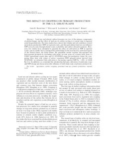
Figure 1: Land Use in Nicaragua in 1983 and 2000
1983
Key: Agriculture Water Scrubland Open-canopy pine forest Closed-canopy pine forest Open-canopy broadleafed forest Closed-canopy broadleaf forest Marshlands Urban
2000
Note: Produced using ArcView and data from MARENA.
7
More important than these somewhat superficial measures, Nicaragua’s history of agrarian reform and tenancy insecurity is typical of Latin America, which has had similarly unbalanced agrarian structures for centuries (Powelson 1988, Thisenhusen 1989). It has followed a similar trajectory as the rest of Latin America from colonization to independence to the present, as an emerging but still somewhat corrupt democracy with an unequal wealth distribution and openness to trade, at least on the regional level. With the proviso that Nicaragua is atypically impoverished, these results should largely be seen as relevant to the rest of tropical Latin America.
1.3. Overview This study has several features which improve upon the existing literature. First, this study’s dataset allows several improvements upon previous micro-level studies (Godoy et a. 2001; Wood and Walker 2000). First, the new cross-sectional dataset from the 2000 agricultural census is three orders of magnitude larger than any used before to answer this question, allowing for more precise estimates. Second, it includes data on an entire country, both reducing the likelihood of having an unrepresentative sample and also including non-frontier regions that are rarely included in deforestation studies but contain a substantial amount of the country’s forest. Third, the study analyzes a broad array of landholding characteristics, apart from landholdinglevel forest cover and tenancy security data, integrated with municipal-level geographical and socio-economic controls. I also decompose the forest by type (primary, secondary, and planted) as well as measure the degree of agricultural intensification and the receipt of credit. These other
8
types of data suggest the mechanisms controlling the relationship between forest cover and tenancy security. Finally, unlike previous work (ie Godoy, et al. 2001), this study has direct measures of tenure status, rather than constructed proxies; it is a study of formal tenure, not informal tenure. Additionally, the use of micro-level data itself has several benefits over regional- or national-level aggregated studies. First, it reduces the likelihood of omitted variables, which plagues Bohn and Deacon (2000), a cross-country study which regresses an index of countrylevel ownership risk on forest stock. For example, although it has little to do with an agricultural landholder’s land use decision, destructive timber concessions may substantially contribute to deforestation and may be more likely in corrupt regimes with insecure land tenancy. Second, the nature of the census data specifically as individually-held agricultural landholdings, not general land use, allows a more focused question and removes potential omitted variables; the dataset does not include timber concessions, national parks, or indigenous communities using slash-andburn agriculture. Third, forestry statistics are notoriously poor. Particularly, the satellite data used on the macro level often used has a resolution inferior to that of a micro-level study and suffers from a computer program’s inherent imperfections in interpreting the color of light reflected as forest cover. This study also checks how representative of the entire country the agricultural dataset by comparing simple bivariate regressions of both aggregated municipallevel data and satellite data of the entire country on tenancy insecurity. Fourth, although measuring insecure tenure with titling is imperfect, this micro-level data removes the need to construct even more arbitrary national-level indices of expropriation risk. Finally, addressing just one country removes the myriad of potential biases introduced from the very different policy
9
environments of multiple countries, any one of which may be an omitted variable correlated with expropriation risk and affecting forest cover. Relatedly, identification, especially with an instrumental variable, is far more plausible within one country. Most importantly, to address the problem of tenancy insecurity’s endogeneity, the study’s instrumental variables approaches take advantage of the natural policy experiment which took place in Nicaragua in the 1980s.9 Previous studies have generally ignored that forest cover and tenure security interact in a simultaneous system, with forest cover affecting demand for title as well as titling affecting forest cover. There are also many omitted variables potentially correlated with both forest cover and tenure security which may cause bias: those untitled tend to be poorer, less well-educated, and in areas with larger amounts of forest.10 The agrarian reform itself, in which Nicaragua redistributed nearly one-third of its agricultural land, accentuated these biases, by giving land with insecure title to the formerly landless poor (Stanfield 1995). I take advantage of two specific policies implemented during the agrarian reform which were exogenous with the proper controls: (1) a policy of increasing redistribution in areas with large amounts of war in order to maintain the loyalties of the people in those regions and (2) an arbitrary division between areas in which expropriation was more and less difficult. Those regions with larger amounts of redistribution have a legacy of insecurity today. This study finds that tenancy insecurity substantially increases forest cover. Specifically, the results suggest that lacking a title increases the fraction of a landholding as forest by 0.15,
9
Both Miceli et al. (2001) and Alston et al. (1999) document the endogeneity of titling. For example, Alston et al. (1996) find that those further from administrative centers—where markets for agricultural or forest products are likely to be—are less likely to have title, due to the increased cost of attaining title at greater distances. They show that having land title is more valuable the closer the land is to the market center, “where competition and private enforcement costs would otherwise be the highest,” due the greater concentration of people with whom to have conflicts. (Alston, et al . 1999, p. 51) 10
10
implying that reducing tenancy insecurity by 10 percent would decrease forest cover on the average agricultural landholding by 8.5 percent.11 I find that the owners of untitled land receive less credit, use less fertilizer, and practice more extensive (versus intensive, or high-input) forms of agriculture, suggesting that tenancy insecurity reduces the returns to deforestation, encouraging landholders to keep the forest cover on their land. This paper proceeds as follows: First, I provide a history of Nicaragua’s experience with agrarian reform. Second, a model with conflicting implications for the impact of tenancy insecurity on forest cover. Third, I describe the individual-level cross-sectional dataset with municipal-controls used in this study. Fourth, I describe the naïve OLS and then the two instrumental variables methodologies used. Fifth, I describe the results. Finally, I briefly conclude.
2. Nicaragua’s History of Agrarian Reform 2.1. 1980s Agrarian Reform & Resulting Insecurity Following decades of undemocratic rule and land concentration among the wealthy, the leftist Sandinista insurgency triumphed over the Somoza dynasty in 1979 and implemented a land redistribution program. Over the ensuing decade while they were in power, the Sandinistas confiscated much of the country’s agricultural land, including the Somozas’ (approximately 20 percent of the country’s agricultural land) and landholdings over a minimum size that the Sandinistas considered abandoned, underused12, or mismanaged.13 The Sandinistas also
11
This marginal effect is calculated using regression (1) of Table 6, given that 38.36 percent of landholdings have no title and 6.76 percent of the average landholding is covered with forest. 12 Underutilized land generally consisted of large tracts of land used for a small herd of cattle); as of 1985, 61 percent of expropriations were justified with underutilization (Stanfield 1995).
11
purchased some land. The Sandinistas then distributed land to multi-family and extended-family cooperatives, individuals, and indigenous communities. Nearly all of the land that the Sandinistas redistributed, either implicitly through permitting land occupations or explicitly after expropriation or purchase, was either given a provisional title or no title at all; this led to the insecure tenancy which persists until the present. The state simply lacked the resources to administer such a massive program, especially after the Contra War (of Iran-Contra fame) started mid-decade. For example, about 3,750 properties, or 70 percent of the total procured from private owners by the Sandinistas, were never legalized as holdings of the state; title was never officially awarded (Stanfield 1995). If title was issued, it was usually issued provisionally because the state did not have legal possession of the land. Even if provisional title was awarded, most of the provisional titles still could not easily be recorded in public registers, since the boundaries and areas of the properties were often not described with sufficient precision, given the hasty nature of the redistribution. According to a 1993 study, “78 percent of the properties investigated remain under the name of the former owners.”14 Finally, even if provisional title was awarded and registered, it could still be challenged by previous owners in courts set up after 1990, when the Sandinistas were voted out of power.15 These challengers include the former owners of the 1,600 properties which were purchased by the Sandinistas, claiming that they were purchased under duress. Thus, the
13
This may seem to create problems for exogeneity. As I explain later on in my methodology section, this does not affect forest cover. 14 Merlet, 36. 15 The review commission had the mandate of reassessing all of the Sandinistas’ property acquisitions and returning those properties that the state acquired unjustly or that third parties illegally occupied. Decisions in favor of former owners, those from whom the land was expropriated, usually allowed the claimant to request the state courts, policy, and army to enforce the eviction of present occupants (Stanfield 1995).
12
combination of challenges, lack of recording in the public registers, and simply untitled land have led to a high degree of tenure insecurity on this land to the present. Table 3: Summary of Land Redistributed in 1980s and Early 1990s Means of Acquisition 1979- Decrees 3, 38, 329: Confiscating land of Somoza and associates 1981- Agrarian Reform Law (Decree 782): Confiscate underused or poorly-managed land 1981- Decree 760: Confiscate abandoned land 1980s- Purchases by Sandinista Government 1980s- De facto occupations Early 1990s- Purchases by UNO Government 1980s- Other means
No. of Properties Area (mz)* 2,000
1,400,000
1,200 252 1,050 510 96 860 5,968
820,000 18,230 196,000 300,000 250,000 88,951 3,073,181
*1 mz = 1.7 acres Note: Due to poor record-keeping, many of these numbers are estimates. Adapted from Stanfield 1995.
As a result of all these conflicts, by 1995 roughly 40 percent of the country’s households found themselves in conflict or potential conflict over land tenure (Stanfield 1995). With the large number expropriations (See Table 3) and redistributions, Nicaragua’s small judicial system was still in 2001, when the data used here is from, sorting through the problems created by the agrarian reform for those who want to have secure tenure, while many others are deterred from obtaining tenure because of the often high costs involved, including multiple visits to Managua without guarantee of success. Even though the government, with the aid of NGOs and United Nations organizations, has been haphazardly establishing titling programs across the country, insecure tenure remains a large problem in Nicaragua today.
2.2. Expectations of Exogeneity Within Communities I make no claims as to the exogeneity of the agrarian reform within communities. The agrarian reform expropriated land from wealthy individuals and redistributed it to the landless 13
poor, who may differ in their land use choices for a variety of reasons, including access to information, credit, and political connections. Given their quasi-socialist ideology, the Sandinistas ostensibly had two sometimes contradictory goals with the redistribution: promoting equality and production (Collins 1986). The first was consistent with their larger goal of maintaining their base of support among the poor and the second was consistent with their larger goal of promoting economic development and maintaining the creation of foreign exchange using the country’s dominant sector, agriculture. To achieve these goals with the redistribution, the government conducted substantial research efforts on the productivity of various types of land, seeking to distribute land of equivalent value to the peasants, while maintaining high agricultural productivity. But the peasants themselves were hardly a random sampling of the population. In my methodology section, I will explain how my approach minimizes the problem of this selection bias.
2.3. Expectations of Exogeneity in Tenancy Security Between Communities Because of the endogenous nature of the agrarian reform within communities, I must find exogenous variation between communities, where there is reason to expect exogeneity in two Sandinista agrarian reform policies, after controlling for geography. First, the government redistributed more land in areas with large amounts of conflict during the Contra War in order to maintain the support of the citizenry, which may have defected otherwise. In areas with high levels of military activity, in the north and south of the country, near the borders from which the insurgents attacked, the government had an additional incentive to redistribute more land in order to keep the support of the people in those regions and prevent defections (Walker 1991; Dillon
14
1991).16 For example, in one of the northernmost regions Esteli, an active war zone, state farms were distributed to such an extent that the state-controlled area was reduced to only 6 percent of the total agricultural land in the region, while the national average was 19 percent (Collinsworth 1988).17 The new owners of this redistributed land were either given provisional titles or no titles at all. Land that was expropriated but not redistributed could easily be returned to former owners, while land that was redistributed entered into a limbo status—with either provisional or no titling. Additionally, there was less rule of law in war-ridden areas, leading to greater numbers of land take-overs, which were not titled, with insecurity lasting until the present. Those areas with larger amounts of land redistribution in the 1980s have a legacy of decreased security in 2000 (Stanfield 1995). Receiving title can be quite costly. Since those areas redistributed in the 1980s were almost always owned by another person, receiving a title could require hiring a lawyer and time in court. Even if the title of the land was not contested, acquiring a title may require trips of many hours to Managua. I talked to some ranchers from the middle of the country who had made the trip three times to receive an uncontested title and still had not received it (Fernandez 2005). Thus, those areas less affected by the war should have a legacy of insecure tenure in 2000 because of the increased amount of redistribution. I argue later in my methodology section that, after controlling for geography and damage to infrastructure, this instrument (which I call hereafter the “war instrument”) is exogenous.
16
It is true that government operations were at risk of rebel attack and dispersing people on newly titled land made them more difficult for the government to police. However, available evidence suggests that large amounts of land redistribution still took place in these areas. 17 Occasionally, the government did take defensive actions which may have reduced land redistribution. For example, in Rio San Juan, the government rounded up individuals to prevent them from aiding the rebels, reducing redistribution. However, the government had only a limited ability to round up civilians and, furthermore, such actions tended to be counter to their goal of keeping the populace on their side.
15
The second exogenous policy shift during the 1980s was the arbitrary division between two regions, in one of which expropriation was easier, resulting in more insecurity. In 1981, the Agrarian Reform Law limited expropriations to farms of over 500 manzanas (2.73 acres) on the Pacific coast and 1000 manzanas in the rest of the country, creating a greater pool for expropriation—and therefore more insecurity—on the Pacific. As with the war instrument, this shift was not completely exogenous—the geography and agrarian structure were different along the Pacific coast than in the rest of the country. However, near the arbitrary division line between these two redistribution treatments, these differences were fairly small—allowing a valid instrumental variables approach (which I call hereafter the “regression discontinuity”) after controlling for geography. The claims to exogeneity of both of these policies is especially strong because most of the redistribution was directed at the municipal- and regional-level during the agrarian reform. In the mid-1980s, MIDIRNA, the Agrarian Reform Ministry, charged the 9 regional offices and later 80 municipal-level zones with administering agrarian reform programs, as Kaimowitz (1989) notes in the aptly-named “The Role of Decentralization in the Recent Nicaraguan Agrarian Reform”.18 These new regional-level structures had substantial budgets and autonomy, promoting adaptation to the two circumstances—war and greater ease in expropriating land— that I propose as my instruments (Kaimowitz 1989).
18
The decision to create 9 regional-level governments contributed to reversing Nicaragua’s long-standing tradition of strong central authority. Until the Sandinista revolution, municipal governments had little authority and autonomy, and despite the division of the country into 16 departamentos, there was no regional government. Fearing US invasion, Nicaraguan carried out the decentralization largely “was carried out to limit the country’s vulnerability to attacks” (Kaimowitz, 396).
16
3. Theory: Model of a Landholder 3.1. A Simple Model In this section, I present a model that shows that: (1) without assumptions on whether investment and land quality are substitutes or complements, the effect of tenancy insecurity on forest cover is ambiguous, and (2) determining the relationship between tenancy insecurity and forest cover can show that investment and land quality are complements. The previous modeling work of Mendelsohn (1994) and Barbier and Burgess (2001) assume that, relative to agriculture, forest cover’s returns are disproportionately in the future; their result is that that tenancy insecurity reduces forest cover. I include this assumption, but also include the effect of tenure security on agricultural investment and productivity, yielding ambiguous theoretical results. Landholder
I assume a rational, profit-maximizing landholder with full information.19
He maximizes the net present value of his future stream of profits ( P ).
Landholding Following Stavins and Jaffe (1990), the landholder lives on a heterogeneous piece of land. In the short-run, the landholding is of fixed size. Potential purchasers of the land value it the same as the current landholder does, so decisions are unaffected by the possibility of selling the land in the future.20 Land is either agricultural or forested; there is no urbanization pressure. Nicaragua has hardly any urban area relative to agricultural area, so this is a reasonable assumption. The fraction of land as agriculture is α (0 <
α < 1), and the fraction of land as forest is 1- α .
19
Given the assumption that all potential landholders value the land the same, the ability to change the size of the landholding should not matter except insofar as there are scale effects, which this model does not consider explicitly. 20 Here, I follow Zwane (2002). This assumption ignores, for example, the effect of migration increasing the value of land.
17
Timing
There are two periods, with each corresponding to five years. The
landholder allocates land between forest and agriculture at the beginning of period one; land allocation stays the same in both periods. The landholders’ land use choices ( α ) are at their equilibrium values. In the past, landholders may have converted from forest to agriculture, reaping the benefits of timber removal and paying the costs of conversion to agriculture, but now markets have achieved their long-term equilibrium. This is possible because deforestation is reversible. This is a plausible assumption, since over half of the forest on Nicaraguan agricultural landholdings is secondary forest, regrown after the original forest was cut down.
Eviction
The landholder discounts the second period because he faces some
probability of eviction (0 < ρ < 1) from the government or other landholders.21 The model could also have included an additional discount factor, but this leaves the results the same, so I excluded it.22
Agricultural land
Agricultural land consists of cropland, planted forest, and
pastureland, which provide profits from the sale of crops or livestock. Planted forest is included since it is intensively and rapidly cultivated, like other crops. The profits from agriculture ( A ) are available in both periods. Profits from agriculture are a function of: (1) the “total quality” of land under cultivation due to geographical characteristics ( Q ), which can be thought of as the sum of a quality index rating for each unit of area; and (2) investments ( I ) in inputs (like fertilizer) and infrastructure Note that ρ is taken as exogenous to α , which may not be the case if certain land uses decrease the likelihood of eviction. 22 Insecure tenure could be seen as equivalent to being impatient. 21
18
(like irrigation systems), given current market conditions.23 Agricultural profits are increasing land quality (
∂A ∂A > 0) and in investment ( > 0). Land quality ( Q ) is a function of fraction of ∂Q ∂I
land devoted to agriculture ( α ), with
∂Q > 0. ∂α
Investment ( I ) is determined exogenously, as a function of the probability of eviction, with
∂I >0. This could function through four channels. First, many landholders are ∂ (1 − ρ )
credit-constrained24; if landholders can demonstrate that they have secure tenure, they can use their land as collateral, which will allow more investment (Alston et al. 1999).25 Second, some investments have liquidity constraints or high transaction costs, especially on a short time scale. For example, if someone were to be removed from his landholding, the liquidity constraints on a barn or soil that he invested in protecting would be almost complete, while the transaction costs of quickly selling a tractor may also be high. Third, the landholder with a higher probability of eviction will choose to invest less because he devalues the future benefits that an investment will bring while valuing relatively higher the costs of the investment. Finally, the landholders with higher probabilities of eviction will spend time and money on defensive tactics, rather than more
23
These current market conditions include the behavior of neighbors. For example, if many neighbors have insecure title and this leads to increased forest cover, then there may be an opening in the market for agricultural goods, inducing increased agricultural land on a titled plot relative to the same plot in an area surrounded by landholders with secure title. See Alston et al. 1999. 24 Although microfinance has spread rapidly, credit is still widely unavailable in rural areas of the third world (Morduch 2000). Credit constraints are especially prevalent in Nicaragua due to the history of bank failures in the country after the Sandinistas left power in 1990; some cities with as many as 30,000 people have no bank. Many still fear putting money in the bank, having lost much of their savings a decade earlier (Guido 2002). 25 The positive effect of tenure security on investment is well-established, though the magnitude is debatable. See Powelson 1988, Alston et al. 1996, and Deininger and Chamorro 2004.
19
productive activities,26 which will reduce investable surplus—often all that is available for investment to a small landholder in a poor country (Field 2003).27
Forested land
Unlike agricultural land, forested land yields profits only in the
second period.28 The landholder must wait for the forest to regrow, through secondary forest at the end of period one through natural forest at the end of period two, at which point it can be harvested.29 Note that this framework is robust to harvesting half of the forest at a time (to maintain windbreaks, for example). The key point is that the landholder must wait for the returns. Profits from forest cover are linear in α , equaling a parameter f > 0 times the amount of land devoted to forest cover (1 - α ).30 In a given area, while agricultural productivity may be highly affected by local geographical conditions, forest productivity is less likely to be affected because forests create their own micro-environments, which make geographical conditions less important. Profits from forest cover are not a function of investment, since investments do not have a substantial direct impact on returns to forests. Few investments other than chainsaws could make forests more productive, and men with chainsaws can easily be “rented” for a portion of the profits from tree-cutting, unlike a warehouse or a tractor (Panayotou and Ashton 1992). 26
For example, a landholder may spend time patrolling rather than planting crops, and conflicts sometimes turn violent. Likewise, conflict with others, which can sometimes turn violent, can also be a substantial cost. See Alston et al. (1999). 27 Microfinance programs are becoming increasingly abundant, but they are hardly ubiquitous. See Alston et al. (1999) and Morduch (2000). 28 Note that results would likely be similar if, following Mendelsohn (1994) and Barbier and Burgess (2001), agriculture were unsustainable, leading to a gradual depletion of soil nutrients and overall quality. The effect would still be that agricultural profits are more forward-loaded than forestry profits. 29 The forest may also provide non-timber resources (like palm leaves and fruits), but those are assumed to be small. 30 This assumption is not perfect. To some extent, returns to forestry will vary with geography. What is important, though, in this exercise, is the change relative to agriculture, which are likely to be far smaller.
20
Figure 2 summarizes the time line. Figure 2: Timing Landholder allocates land between forest (1 − α ) and agricultural ( α ) cover
Landholder receives agricultural profits ( A(•) )
Landholder receives agricultural profits ( A(•) ) and forest profits ( (1 − α ) ⋅ f ) if not evicted Possibility of Eviction
Time Period 1
Time Period 2
The landholder will optimize his land use choice according to the following equation: (1) max P = A(Q (α ), I (1 − ρ ) ) +(1 − ρ ) ⋅ [ A(Q (α ), I (1 − ρ ) ) + (1 − α ) ⋅ f ] 31, α
where all functions are twice continuously differentiable and take and yield only values in the reals. Also, assume that an interior solution exists.
Proposition 1: The effect of property rights on forest cover,
and
∂α * , is of ambiguous sign, ∂ (1 − ρ )
∂2 A , the degree of substitutability or complementarily between land quality and ∂Q∂I
investment, determines the sign. The following result shows conditions with which to show that the sign is ambiguous: by the Monotone Selection Theorem32, (A) If
∂α * ∂2P > 0 , then ≥ 0 ; and (B) if ∂ (1 − ρ ) ∂α∂ (1 − ρ )
Since Q and I are monotone functions of α and (1- ρ ), respectively, I could suppress the intermediate functions, but I am not for clarity of exposition. 32 Thanks to William Woolston for suggesting the use of this theorem. 31
21
∂α ∂2P ∂ 2α * < 0 , then ≤ 0 .33 Hence, determining the sign on depends critically ∂ (1 − ρ ) ∂α∂ (1 − ρ ) ∂ (1 − ρ ) on the sign of
∂P . I now show that theory cannot give clear predictions on the sign of ∂α∂ (1 − ρ )
∂P . ∂α∂ (1 − ρ ) Taking the cross-partial of (1) yields: (2)
∂2P ∂ 2 A ∂Q ∂I ∂A ∂Q = (2 − ρ ) ⋅ ⋅ ⋅ + ⋅ −f ∂α∂ (1 − ρ ) ∂Q∂I ∂α ∂ (1 − ρ ) ∂Q ∂α 14444 4244444 3 14243 (i )
( ii )
We know that term (ii) of (2) is positive, since taking the first-order condition of (1) and rearranging yields: (3) f =
(2 − ρ ) ∂A ∂Q ⋅ ⋅ (1 − ρ ) ∂Q ∂α
Since ρ < 1, we know that f >
∂A ∂Q ⋅ . This makes sense because per-period marginal ∂Q ∂α
profits from forestry ought to be higher to compensate for only being available in the second period.
P ought technically to be redefined as a function only of (1 − ρ ) and α ; however, for clarity of exposition, I am keeping the same function. The statement of the theorem requires that P(α , (1 − ρ )) has increasing 33
differences, which is equivalent to the conditions on the cross-partial, assuming continuous differentiability. Likewise, the theorem’s result is that (1 − ρ ) > (1 − ρ )' implies that α ≤ α ' at equilibrium values of α * , which is equivalent to
∂α * ≥ 0 , assuming continuous differentiability. These results reverse for the negative; this ∂ (1 − ρ )
can be seen by noting that all the result for increasing differences applies when simply taking the negative of (1 − ρ ) .
22
However, term (i) of (2) has an unclear sign, since there is no assumption on the cross∂2 A ∂2 A . Different assumptions on will then yield different signs on partial term ∂Q∂I ∂Q∂I ∂2P ∂ 2α * (and hence on , by the Monotone Selection Theorem). ∂α∂ (1 − ρ ) ∂ (1 − ρ )
Part (A) of the Monotone Selection Theorem result requires that: ∂A ∂Q ⋅ ∂ A ∂Q ∂α > , (4) ∂Q ∂I ∂Q∂I (2 − ρ ) ⋅ ⋅ ∂α ∂ (1 − ρ ) f −
2
which is found by setting the right-hand-side of (2) as greater than zero. Since f >
∂A ∂Q ⋅ ∂Q ∂α
∂2 A and the denominator of (4) is greater than 0, we know that > 0 is a necessary (but not ∂Q∂I
sufficient) condition for part (A). Thus,
complements, implies that
∂2 A > 0, the equivalent of Q and I being ∂Q∂I
∂2P > 0 . This occurs with Cobb-Douglas functions, for ∂α∂ (1 − ρ )
example. Likewise, part (B) of the Monotone Selection Theorem result requires that: ∂A ∂Q ⋅ ∂ A ∂Q ∂α (5) < , ∂Q ∂I ∂Q∂I (2 − ρ ) ⋅ ⋅ ∂α ∂ (1 − ρ ) 2
f −
23
which is found by setting the right-hand-side of (2) as less than zero. Since, as before, the right∂2 A ∂2 A . Thus, < 0 is a sufficient (but not hand-side is positive, we cannot assign a sign to ∂Q∂I ∂Q∂I
necessary) condition for (B) to be satisfied. If Q and I are substitutes or even complements such that (5) is satisfied, then (B) will be satisfied. □
This model then is theoretically ambiguous since either condition on
∂2 A is plausible, ∂Q∂I
so the relationships between tenancy insecurity and forest cover must be determined empirically. However, this model does show that the degree to which land quality and investment are substitutes or complements determines the effect of property rights on forest cover.
Proposition 2: If
∂2 A ∂α * > 0. Total land quality, Q , and investment, I , are > 0, then ∂ (1 − ρ ) ∂Q∂I
complements. Taking the contrapositive of part (B) of the Monotone Selection Theorem result yields: if ∂ 2α * ∂2P > 0 , then ≥ 0 . By reasoning similar to that above, we know that ∂ (1 − ρ ) ∂α∂ (1 − ρ )
∂A ∂Q ⋅ ∂ A ∂Q ∂α ≥ > 0, (6) ∂Q ∂I ∂Q∂I (2 − ρ ) ⋅ ⋅ ∂α ∂ (1 − ρ ) 2
which shows that
f −
∂2P ∂2 A > 0 if ≥ 0 .□ ∂α∂ (1 − ρ ) ∂Q∂I
24
An analogous result is not possible for
∂ 2α * < 0 , since that would depend upon a ∂ (1 − ρ )
sufficient, not a necessary, condition on the relationship between
∂2P ∂2 A and . ∂Q∂I ∂α∂ (1 − ρ )
3.2. Graphical Rendition of Model We are left then with possibly two conflicting implications for the effect of tenancy insecurity on forest cover. A high probability of eviction will disproportionately devalue forest because forests’ returns are disproportionately in the future. Thus, high eviction rates will decrease forest cover. This is the “commons effect,” term (ii) in (2),
∂A ∂Q ⋅ − f , which is the ∂Q ∂α
marginal cost of having agriculture for a change in (1 − ρ ) , when ignoring the effects of technology.34 However, a high probability of eviction will also change the composition of the agriculture, discouraging investment, making agriculture less valuable relative to forestry, which is unaffected by investment. This is the “investment effect,” term (i) in (2). Since
the sign of the investment effect depends upon the sign of
∂I > 0, ∂ (1 − ρ )
∂2 A ∂2 A . If < 0, then the ∂Q∂I ∂Q∂I
∂A ∂Q ⋅ , the first period marginal profits, equal to ∂Q ∂α ⎡ ∂A ∂Q ⎤ the “marginal cost” of having agriculture, (1 − ρ ) ⋅ ⎢ f − , the discounted second period marginal profits. ⋅ ∂Q ∂α ⎥⎦ ⎣ This is what one gets when taking the first-order condition of (1). Increases in (1 − ρ ) , having more secure tenure, 34
Think of setting the “marginal benefit” of having agriculture,
will increase the marginal cost of having agriculture, and forest cover will increase.
25
investment effect is negative, the same as the commons effect. If
∂2 A > 0, then the investment ∂Q∂I
effect is positive, contrary to the commons effect.
I present these two effects in Figures 3 and 4, in which α * is determined by the point at which the line for the marginal returns from forest cover crosses that for agricultural cover. For ∂2 A > 0). I also assume the sake of exhibition in graphical analysis, I assume the latter case ( ∂Q∂I
that
∂ 2Q < 0, the relationship between land for agriculture and total land quality is concave; this ∂α 2
will almost certainly be the case, since the landholder will move to less desirable land35 with more agriculture. Figure 3, the commons effect, presents the view found in Mendelsohn (1994) and Barbier and Burgess (2001). Higher expropriation risk leads to higher effective discount rates. Because forestry’s returns are disproportionately in the future, higher effective discount rates disproportionately discount forest’s value, with agriculture’s value decreasing from line A to line B with greater insecurity, but forest cover’s marginal value decreasing a larger amount from line C to line D. Thus, forest cover is more attractive in a secure-tenancy regime, demonstrated below by the larger amount of forest with higher marginal returns than agriculture (more of C over A than B over D) with secure tenancy than with insecure tenancy. This theory predicts that landholders with insecure tenure, or a high risk of expropriation, will have less forest.
35
For example, as the landholder moves to land further from road, with more of a slope, or with lower soil fertility (Lutz et al. 1994). Also, with little forest left, there will be less protection from wind and water erosion.
26
Figure 3: The Commons Effect: Two-Period Profits Discounted by Expropriation Risk, Holding Technology Constant
Relative Marginal Returns
Percentage of land as forest ( 1 − α ) 0 1 Agriculture: Secure Tenure (low ρ ) A Forest Cover: Secure
Agriculture: Insecure Risk (high ρ )
B Forest: Secure Tenure
C Forest Cover: Insecure
1
Forest: Insecure Tenure
Larger difference for forest
D 0
Fraction of land as agriculture ( α )
Figure 4 shows the investment effect when investment and land quality are complements, occurring simultaneously with the commons effect. Unlike the previous model, which assumes that the type of agriculture stays the same regardless of tenancy security, this diagram looks precisely at this change in the composition of agricultural land. Also unlike the previous diagram, it does not include the effect of increased expropriation risk in discounting future returns. Rather, it only includes the effect of tenancy insecurity on investment behavior. Because of the greater likelihood of capturing future benefits from investment in a securetenancy regime, landholders will invest more, increasing agricultural productivity by changing from more extensive to more intensive agriculture—increasing agricultural returns from line B to line A. Returns to forest, on the other hand, are not directly affected by investment and are the same in both high-risk and low-risk regimes, at line B. Thus, increases in agricultural
27
productivity increase the returns to agriculture—and, therefore, deforestation. The investment effect predicts that landholders with insecure tenure, or a high risk of expropriation, will have more forest.
See Appendix F for additional considerations of the model for empirical analysis. Figure 4: The Investment Effect: Two-Period Profits with Effect of Changed Expropriation Risk on Technology, but Not on Discounting
Relative Marginal Returns
Percentage of land as forest today ( 1 − α ) 0 1
Forest Cover: Secure
A
Intensive Agriculture: Secure Tenure (low ρ )
B
Extensive Agriculture: Insecure Tenure (high ρ )
C
Forest: Secure & Insecure Tenure
Forest Cover: Insecure
1
0
Percentage of land as agriculture ( α )
4. Data This study’s independent variables come from Nicaragua’s 2001 Agricultural Census. The National Institute of Statistics and Censuses (INEC) and the Ministry of Agriculture and Forestry (MAG-FOR) conducted the census in March 2001 on the agricultural year from May 1, 2000, to April 30, 2001. All 199,549 agricultural holdings in the country covering 6,254,514 ha were surveyed, excluding kitchen-gardens in urban areas. These landholdings—cooperatives,
28
commercial enterprises, and individual landholdings—constitute a little over half (52 percent) of Nicaragua’s land area. The survey includes 75 percent of total land area for non-frontier areas and 40 percent for frontier areas, with departments ranging from 22.1 percent36, where there are large forest reserves and Indian reservations to 92.3 percent37 coverage in a well-developed agricultural area. Landholdings range from less than 1 manzana to 35,000 manzanas. The majority of the area falls between 10 and 500 acres, while the majority of the landholders have under 50 acres. (See Table 4.) Nearly 1/3 of the landholdings’ land area consists of natural pasture, while 14 percent consists of forests. (See Table 5.)
Table 4: Area of Landholdings by Size size (in number of manzanas) mean median landholders 0 to 1 0.72 0.75 18,082.00 1 to 5 2.70 2.50 41,183.00 5 to 10 6.63 6.25 27,190.00 10 to 50 22.97 20.00 66,008.00 50 to 100 63.98 60.00 24,656.00 100 to 500 175.32 150.00 20,482.00 500 to 1,000 639.08 600.00 1,432.00 1,000 to 5,000 1,590.54 1,300.00 493.00 5,000 to 10,000 6,275.96 6,000.00 15.00 10,000 to 40,000 19,098.09 15,491.00 8.00 Total 44.78 12.00 199,549.00 Note: Lower bound inclusive, upper bound exclusive 1 manzana = 2.73 acres
36 37
percentage of area 0.15 1.24 2.02 16.97 17.65 40.19 10.24 8.78 1.05 1.71 100.00
In RAAN, the Northern Autonomous Region. In Granada.
29
Table 5: Make-Up of Census's Land
Annual crops Permanent crops Fallow Natural pasture Planted pasture Infrastructure Forest Natural Secondary Planted Other Total
Percentage of Total Percentage Area of Forest 10.72 4.73 18.99 32.82 14.90 1.13 14.22 5.02 42.32 7.76 54.61 0.44 3.07 2.49 100
Those census questions relevant to this study include: tenure, size of holding, education, investment in various farm technologies and agricultural inputs, and land use (forest cover, type of crop, type of grazing, etc.). Those with no secure title, as described in this study, have no title at all, are in the process of legalizing their title, or have a provisional agrarian reform title. The individual-level disaggregates by type: natural, secondary, and planted. This disaggregated forest data is particularly useful because we may expect different effects of land tenancy on different types of forest; for example, planted forest is clearly an investment, while natural forest may or may not be. Such a large individual-level dataset with such detailed land use data is unique in the literature on tenure security and deforestation. As mentioned previously, this study measures the effect of formal tenure security using possession of a public title. By 2000, conflicts remained over lands without secure title and even some with public title (Merlet 2000). Thus, in some cases, landholders may respond that they have publicly-recognized title, despite the existence of others who claim to have a document of equal legitimacy; in the econometrics, this may reduce the effect of “tenure insecurity” on forest
30
cover, since some of those in the titled category may also be insecure. More importantly, though, by 2000, Nicaragua had been stable for a decade; there was little fear of government expropriation (Merlet 2000). In contrast to the 1980s, when all lands seemed fairly insecure, there is now a substantial difference in tenure security between titled and non-titled land. This measure also should not be seen as a comparison of having complete and no tenure security, since many without title have forms of informal title. For example, officials from the United Nations Development Program estimate that about 60 percent of those in the rural region of Esteli do not have legally recorded title, instead functioning under traditional inheritance schemes.38 These problems in my measurement of tenancy security should bias the impact of tenancy on forest cover toward zero. Additionally, there may be problems of response to such questions on census: especially the more economically vulnerable may be reluctant to admit to a government worker that they lack title for fear that the government may come take their land away from them. While this factor would reduce the overall response rate for lacking title, it is unlikely that this would bias the results since I control for socio-economic status. This study also uses Geographical Information Systems (GIS) data associated with the Ministry of Environment and Natural Resource’s 2004 “Atlas Forestal.” The atlas provides high-resolution geographical data on elevation, slope, precipitation, soil texture, and temperature. It also provides socio-economic information on poverty levels in the year 2000 and road density in the mid-1990s. Finally, the atlas contains forest cover data resolved to 30 square meters for 1983 and 2000, a useful check of robustness to the census forest cover data as well as measure of
38
Ibid, 21.
31
initial conditions. This data was processed using Arc geographical software and divided into Nicaragua's municipalities; the data that appears in the regression is constructed by multiplying the proportion of a municipality’s land covered by a particular value (like an annual rainfall of 1000 mm) by the value, and then adding these products together. Finally, I also incorporate municipal-level data on rural and urban population density in 1995, as well as geographical coordinates, from Nicaragua’s National Institute of Statistics and Censuses (INEC). See Appendix B for correlations and Appendix C for summary statistics.
5. Methodology 5.1. Naïve Strategy: Model To determine the impact of tenancy insecurity on forest cover in 2000, I use ordinary least squares regressions on only the individual landholders in the dataset, excluding cooperatives and commercial enterprises, which may operate under very different systems. I use the following specification39: (6)
f i = α + β wi + δcm + γd i +ε i
where f is the fraction of land covered by forest or components of forest (natural, secondary, and planted) in 2000, w is the fraction of a landholding without title (usually 0 or 1, but possibly between if the landholder has multiple parcels), c is a vector of control variables at the municipal
39
I follow Stock and Watson (2003) and use heteroskediastic-robust standard errors because there is no reason to think that the data would be homoskedastic. However, there is little reason to think that the heteroskedasticity would operate primarily at a particular level—municipal, size, etc.—so the general robust standard errors are superior to clustered standard errors.
32
level, and d is a vector of individual-level control variables. Municipal-level controls are poverty level, distance from the capital Managua, rural and urban population density, road density, elevation, mean annual temperature, slope, and soil quality, and precipitation. Individual-level controls are log area of landholding and educational status. See Appendix G for an explanation of why each control is used.
5.2. First Instrumental Variables Approach: Entire Country If these covariates fail to control for any unobserved heterogeneity correlated with tenancy, then estimating an unbiased coefficient on the endogenous tenancy variable requires exogenous variation. There are several reasons that we would expect such omitted variables. First, landholders may deviate from the assumption of a rational, perfectly-informed actor. For example, a lazy individual may neither cut down trees nor attain title. Or an individual may be myopic, cutting down every tree since he cares none for the future, while not investing in a title. Second, unobserved micro-geographic variables may cause both less titling and less forest. For example land that is dry or on a hillside may not be desirable for farming, so a landholder may leave the trees. However, because of the land’s lower value, he may not bother attaining a title. Third, the agrarian reform itself assigned land to a certain type of person, usually poor, which may be correlated with forest cover; it is possible that the measure of education above does not adequately control for this omitted variable. Perhaps more importantly, forest cover and tenancy security may simultaneously cause each other. For example, at some points in Nicaragua’s past, before the 1980s, the government
33
granted title partly dependent upon demonstrating use of the land through clearing the forest. Thus, deforestation may increase the availability of secure tenure on the supply side. Alternatively, deforestation may increase the demand for titling on the demand side. Landholders with forest are more vulnerable to land invasions from neighbors since their land looks underutilized; recognizing that they lack the informal tenure security provided by agriculture, they may have a higher demand formal title (Alston et al. 1999). Using instrumental variables is one way to well-identify the coefficient on the endogenous tenancy variable. For an instrument (Zi) to be valid, it must satisfy two conditions: (A) corr(Zi, , Xi) ≠ 0, and (B) corr(Zi , ε i ) = 0, for the equation Yi = β 0 + β1 X i + ε i , in which X is the endogenous variable or variables. To find a relevant instrument, I take advantage of Nicaragua’s unique history. In the mid-1980s, the Sandinistas responded to the war against the counterinsurgency by increasing the amount of land redistribution in order to maintain the support of the locals and discourage them from aiding the rebels. Since the insurgency was mounted from Nicaragua’s borders, I have two instruments as good measures of the extent to which the war affected the municipality: presence in a department adjacent to the southern border and also the northern border. To increase the strength of these regional-level variables, I interact multiplicatively location adjacent to the northern and southern borders with the landholder’s educational status. Educational status is relevant to titling status because those who received land during the agrarian reform were primarily those who were in need of land, the poor. Those who had political connections may also have received more land. Since my measure of socio-economic status is educational status, I would expect the least amount of redistribution among the rich,
34
those with post-secondary degrees. Depending on whether the effect of political connections or the effect of need matters most, I would expect either the lower socio-economic group (without any education) or the intermediate group (primary or secondary education) to have the most redistribution—and, therefore, tenancy insecurity. The interaction with educational attainment is exogenous because I also separately control for education in both the first and second stages.40 Unless individuals with the same educational status differed between the north and the south in some way that affected forest cover, other than a different likelihood of receiving land, interacting location adjacent to a border with educational status will introduce no bias. Table 6 compares the mean values for departments adjacent to and not adjacent to the borders. Conveniently, the number of landholdings is approximately the same in both regions. Approximately 50 percent more landholdings are insecure in border regions than non-border ones. Landholdings are approximately the same size on average. The center of the country also has substantially less forest and higher population densities. Geographically, the main difference between the two regions is soil type. The landholders in the center of the country have somewhat higher educational attainments. There may be several objections to these instruments. Certainly, without geographical controls, the instrument would not be exogenous. Most differences in means in Table 6 are significant, so it is clear that the instrument is only conditionally exogenous. 41 For example, the
40
The interaction captures two effects, neither of which is correlated with the errors after controlling for educational status itself. First, it captures the absolute increase in the number of those of lower educational status who receive land; they were the most likely to receive land during the redistribution, so increasing the percentage of the population to receive land will result in a disproportionately high increase in the absolute number of uneducated who receive redistributed land. Second, it captures the relative increase in the educational strata which receive more land in the war-ridden areas. It is unclear what the marginal group is which would be more likely to receive land in areas with more redistribution, assuming that there is any affect at all. In any case, the two effects are indistinguishable. 41 The variables for which the means are not significantly different are the receipt of credit, elevation, and slope.
35
northern part of the country is mountainous, where agriculture is less viable and one would expect both more forest cover and that the rebels would have more easily evaded government forces, making government control—and land redistribution—more difficult.
36
Table 6: Means for Border and Non-Border Departments for War Instrument observations
Non-Border Border 94250.00 102658.00
Dependent Variables
Non-Border Border Controls: Municipal-Level precipitation (m/year)
fraction total forest fraction natural forest fraction secondary forest fraction planted forest
0.04
0.09
(0.13)
(0.19)
0.01
0.04
(0.06)
(0.13)
0.03
0.05
(0.10)
(0.14)
0.004
0.002
(0.04)
(0.03)
Endogenous Independent Variables fraction without title 0.30 log area (mz) warehouse ownership Mechanisms receipt of credit (1 = yes, 0 = no) use of fertilize (1 = yes, 0 = no) ownership of tractor (1 = yes, 0 = no) cropland/(cropland + pastureland) fraction cropland permanent cropland / total cropland fraction pastureland planted pastureland / total pastureland fraction fallow
permanent workers temporary workers
(0.49)
2.69
(1.72)
(1.58)
0.07
0.06
(0.26)
(0.23)
0.15
0.15
(0.36)
(0.35)
0.56
0.41
(0.50)
(0.49)
0.09
0.07
(0.29)
(0.26)
0.62
0.62
(0.40)
(0.37)
0.44
0.41
(0.36)
(0.33)
0.29
0.28
(0.38)
(0.34)
0.29
0.27
(0.34)
(0.32)
0.25
0.32
(0.38)
(0.43)
0.14
0.17
(0.24)
(0.23)
3.29 (2.36)
0.63
0.47
(2.89)
(2.68)
2.25
2.83
(14.02)
(12.65)
area (mz)
slope/100 ( percent) fine sandy soil clay soil
2.26
(2.13)
temperature (C)
0.46
(0.45)
Labor Characteristics: Individual-Level members of household working 2.91
elevation (km)
38.38
44.61
(120.35)
(102.94)
sandy soil heavy clay soil high poverty distance from Managua (degrees) rural population density (persons/sq km 1995) urban population density(persons/sq km road density (km road/km^2) 1983 forest cover Controls: Individual Level no education can read and write primary education secondary education post-secondary education
1.45
1.77
(0.42)
(0.70)
0.40
0.44
(0.25)
(0.33)
24.24
23.74
(1.34)
(1.57)
0.29
0.28
(0.12)
(0.12)
0.37
0.18
(0.32)
(0.26)
0.06
0.02
(0.14)
(0.08)
0.35
0.66
(0.37)
(0.41)
0.10
0.05
(0.15)
(0.14)
0.38
0.67
(0.47)
(0.46)
0.99
1.76
(0.61)
(0.66)
78.11
26.71
(0.24)
(0.02)
99.39
15.02
(0.25)
(0.03)
0.02
0.01
(0.06)
(0.02)
0.44
0.69
(0.23)
(0.23)
0.40
0.45
(0.49)
(0.50)
0.05
0.06
(0.22)
(0.24)
0.39
0.41
(0.49)
(0.49)
0.09
0.06
(0.28)
(0.23)
0.07
0.03
(0.25)
(0.16)
Standard deviation in parenthesis.
Likewise, the northern and southern parts of the country have more forest than the rest of 37
the country because they are further from the capital Managua in the center of the country. However, looking at a national map of Nicaragua’s forest cover (see Figure 2), it becomes readily apparent that the agricultural frontier forms a semi-circle with Managua as its center; therefore, controlling for distance from Managua should be an adequate control for the less developed parts of the country, which are likely to have both less secure tenancy and more forest cover. Controlling for distance from Managua means that the instrument, rather than working along a strict north-south axis, works outwardly in concentric circles radiating from Managua. Likewise, controlling for the slope and elevation using the municipal-level data from the Nicaraguan Environmental Ministry should remove the bias of the disproportionately mountainous northern regions, for example. The comprehensive set of geographical controls used should remove any bias introduced by other such endogeneity problems. Second, one may argue that the possibility of greater amounts of redistribution spurred large migrations into these regions—or alternatively, that the war spurred large migrations out of these areas. In the former case, that redistribution encouraged migration into these areas, given certain initial conditions then, areas with larger amounts of redistribution and insecurity would appear to have less forest, assuming that higher population densities lead to reduced forest cover. There were substantial migrations during the 1980s, but they were largely into cities (Walker 1991). Furthermore, controlling for rural and urban 1995 population density should control for this bias. In addition, I run 8 permutations of municipal-level regressions of absolute as well as percentage change in both total as well as rural population density between 1971 and 1995, both controlling and not controlling for distance from Managua (since areas at the frontier have more space for expansion, they may have had larger absolute increases in density), attempting to test if
38
border regions did indeed experience larger migrations in or out. Each of these regression yields an insignificant coefficient on the municipality being in border region, suggesting that migration does not introduce a substantial bias. A third concern is errors-in-variables bias: that the distance from the borders measures something other than the effect of the war that is correlated with forest cover, even after geographical controls. For example, if Honduras or Costa Rica (Nicaragua’s neighbors to the north and south, respectively) represented significant export markets for Nicaraguan wood and transport costs were significant, then areas of Nicaragua near the borders might have higher forest cover due to the higher value of timber products (Foster and Rosenzweig 2003). However, Nicaragua is a small country; the entire length can be driven in a matter of hours. While an insurgency predominantly on foot may be impeded by distances, trade likely is not. Fourth, errors-in-variables bias would also be problematic if there were substantial cultural differences between the different regions that were not controlled for either by distance from the capital or geographical covariates. While the western half of the country has been controlled by the Spanish and their descendants since the 16th century, the eastern half was under English control for a substantial portion of that time, and it still has substantial indigenous communities. However, cultural differences are not worrisome because cultural and developmental divides in Nicaragua are predominantly between the east and the west, not the north and the south (Enriquez 1991; Merlet 2000). Fifth, war likely increased damage to infrastructure, which could discourage agricultural intensification—and thereby decrease the returns to deforestation. In fact, state farms were a primary target of the counterinsurgents (Collinsworth 1988). Consequently, given that it is
39
possible that this infrastructure damage lasted until 2000 in the war-ridden areas, I include a measure of infrastructure (fraction of landholding devoted to infrastructure) as an endogenous variable in the instrumented regressions. Sixth, redistributed land is likely to be smaller relative to the rest of the land because the predominant mode of redistribution was taking large landholdings owned by the wealthy and redistributing that to the poor in smaller holdings. We would expect that in the non-war regions where there was more redistribution, the size of the landholding of the wealthiest would be most reduced. Thus, the size of the landholding is another endogenous variable and I instrument for it, along with fraction of land without title and fraction of land devoted to infrastructure. Having suggested that the instrument is both relevant and exogenous, I run a two-stage least square regression, on OLS regressions, with the following specification in the first stage: (10) X 1i = ς 1 + π 1 Z i + η1 d i + ψ 1c m +ε 1i (11) X 2i = ς 2 + π 2 Z i + η 2 d i + ψ 2 c m +ε 2i (12) X 3i = ς 3 + π 3 Z i + η 3 d i + ψ 3 c m +ε 3i where X 1i is the fraction of the landholding without title, X 2i is the log of the size of landholding, X 3i is the fraction of landholding devoted to infrastructure, Z is a vector of instruments interacting educational status with presence at the northern and southern borders, d is a vector of individual level educational controls, and c is a vector of municipal-level controls. Having done regressions (10)-(12), we now have predicted values for the three endogenous variables: (13) Xˆ 1i = πˆ1 Z i + ηˆ1 d i + ψˆ 1c m
40
(14) Xˆ 2i = πˆ 2 Z i + ηˆ 2 d i + ψˆ 2 c m (15) Xˆ 3i = πˆ 3 Z i + ηˆ3 d i + ψˆ 3 c m , where Xˆ 1i are the predicted values for being without title, Xˆ 2i are the predicted values for size of landholding, Xˆ 3i are the predicted values for fraction of landholding devoted to infrastructure, and the other variables are the same as above. The second stage is then: (16) f i = α + β 1 Xˆ 1i + β 2 Xˆ 2i + β 3 Xˆ 3i + γd i + δc m +u i , where the symbols are the same as in the OLS, and Xˆ ni are the values predicted by the first stage. Although Local Average Treatment Effects (LATE) may seem like a concern, the identified effects actually correspond closely to average treatment effects for poor landholders. The fact that much of the land that was redistributed was expropriated on the basis of its being “underutilized” may arouse suspicion that “underutilized” equated with being covered by more trees than most agricultural land. This could mean that the instrument would pick up the effect only of redistributing marginal or highly tree-covered land. Admittedly, the location of these underutilized plots was not completely random and probably was correlated with more marginal land qualities. To see how significant this concern should be, I interviewed the Minister of Agrarian Reform during the 1980s, Jaime Wheelock Ramon. When asked, “Was the land that was expropriated and then redistributed more or less likely to have forest?” Wheelock responded, “No. Generally, the land that was underutilized was brushland that had only a few cattle on it, but not more trees” (Wheelock 2005). Often underutilized plots were adjacent to plots of
41
intensive agriculture with the same land qualities. The owners had just left because of the war, and the land was likely farmed relatively recently. Likewise, the redistributed land may have been of a particular type because of the size of the landholdings which were redistributed. After 1981, only large plots of over 500 manzanas on the Pacific Coast and over 1000 manzanas elsewhere were expropriated and then redistributed. According to Wheelock, the only exception to this type of redistribution occurred when land was occupied by squatters, which would mitigate this effect somewhat. Since this study shows that larger plots of land in 2000, ceteris paribus, have a higher fraction of forest cover, once that land was redistributed, those with insecure tenure on the new plots may have had a larger amount of forest as their initial condition; this is problematic if forest cover in the 1980s matters for forest cover in 2000. However, an even larger amount of land associated with the Somoza dynasty was expropriated before 1981, which consisted of very large landholdings with highly intensive agroexport agriculture and few trees (Wheelock 2005). Though a smaller proportion of the Somozas’ land was redistributed than the post-1981 land, the Somozas’ land amounted to a massive 20 percent of the country’s agricultural land. It is unclear which of these two effects dominates, but that they go in opposite directions offers some hope that they cancel each other out somewhat.42 However, the group which benefited is not representative of Nicaragua’s population; it is representative of the rural poor, and the result should be seen as such. In any case, this is primarily the group of interest to studies on deforestation, since it is the group believed to be the proximate cause of much of the deforestation in the world today (Alston et al. 1999). 42
The former Somoza land has since been divided up between pervious owners, ex-soldiers, and former workers of the state enterprises in roughly equal proportions (Stanfield 1995).
42
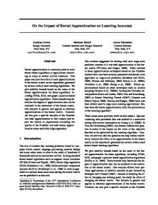
Figure 5: Tenancy Insecurity by Municipality
Note: Generated using ArcView with 2000 Agricultural Census data
43
5.3. Second Instrumental Variables Approach: Regression Discontinuity 5.3.1. Forest Cover I also undertake a second instrumental variables approach, using regression discontinuity as a test of robustness for the first approach. I take advantage of the arbitrary line drawn between two similar areas in which two different policies were implemented: to the west, land could be expropriated with a minimum of 500 manzanas, and, to the east, with a minimum of 1000 manzanas, creating a larger pool of land to expropriate in the west—and, therefore, more expropriation and subsequent insecurity. Therefore, using the same methodology described above, I look only at the 17 municipalities—9 on the west and 8 on the east—adjacent to the line dividing these two policy treatments. This second approach is particularly valuable as a test of whether the results are merely a frontier phenomenon because these 17 municipalities are entirely in non-frontier areas. Table 7 compares the mean values for each of the two regions. Conveniently, both have about the same number of observations. They both have substantially less forest than the country as a whole, particularly for natural forest. The western side has slightly more forest. The intensification measures are not uniformly higher in either region. A substantially larger number of landholders on the western side lack title: 45 percent versus 33 percent. The eastern side is substantially more municipal-level impoverished, reflecting potentially different market conditions; educational attainment in both regions is remarkably similar, though, suggesting that large socio-economic differences do not exist. The east also has a substantially higher elevation.
44
As with the first instrument, geographic controls are essential, since most of the means are significantly different between the east and the west.43 The only instrument in this case is geographical location—to the west or to the east of the discontinuity. Therefore, the area of the landholding cannot be endogenous—or there would be more endogenous variables than there are instruments. If I looked at the entire census of landholdings, size would be endogenous because landholdings between 500 and 1000 manzanas were expropriated and redistributed on the western side, while they were not on the eastern side; since the fraction of forest cover tends to increase with the size of the landholding, including the observations would make the instrument correlated with forest cover. To remove this endogeneity, I remove all landholdings—only 2 percent of the total—larger than 500 manzanas. This should not introduce any bias because the observations removed are equivalent on both sides of the discontinuity; the result is that the meaning of the results is a bit more limited than the war instrument, limited only to lands which could have been redistributed and could not have been expropriated. Considering the area of the landholding as exogenous also requires the assumption that, in redistributing land, the Sandinistas did not consider the amount of forest on the land when dividing up expropriated parcels. For example, if they thought that areas with a large number of trees were particularly valuable, they may have assigned the person who received that part of the land a smaller plot, in the interest of fairness—making the size of the landholding endogenous. Alternatively, if they viewed forests as wasted land, possible given their focus on increasing
43
The exceptions are fraction pastureland, number of members of the household working, number of permanent workers, distance from the capital, rural and urban population density, 1983 forest cover, and primary and postsecondary education.
45
agricultural production in the short-term to produce foreign exchange, they may have done the opposite. Given that the direction of the bias is unclear and Minister Wheelock pointed out that the amount of forest on this land was very small to begin with, whatever effect forest cover had on the size of the landholding was likely minimal. It is also possible that, given the greater amount of land available for redistribution available on the western side of the line, the average redistributed landholding there would be larger—and that size of landholding would be endogenous even after removing landholdings over 500 manzanas. A simple test shows that the insecure landholdings are not any larger on the western side of the discontinuity today (t = 0.08). While this is not a definitive test, there is no reason to believe that landholders on the western side would have disproportionately titled larger landholdings relative to the eastern side, especially given the Sandinistas’ devotion to equality (Collins 1986). So we may take this structure today as a reflection of the policies of the 1980s and proceed with area as an exogenous control variable. Another objection to this instrument may be important unobserved cultural, historical, or other differences between the regions. Indeed, the line drawn between the two policy areas is not completely arbitrary; it follows departmental boundaries. These divisions themselves, however, are essentially meaningless. Except for the brief period in the mid-1980s during the agrarian reform, a departmental government has never existed in Nicaragua (Enriquez 1991). Only in the late 1990s did the national government begin to devolve limited powers to the municipalities, which are severely hampered by a lack of funds (Merlet 2000). Areas so close are unlikely to have substantial cultural differences, and both areas have had common histories as part of the Spanish empire and then part of independent Nicaragua.
46
Table 7: Means for Western and Eastern Parts of Regression Discontinuity West East number of variables 9322.00 9468.00 Dependent Variables fraction total forest fraction natural forest fraction secondary forest fraction planted forest receipt of credit use of fertilize ownership of tractor ownership of warehouse cropland/(cropland + pastureland) fraction cropland permanent cropland / total cropland
fraction pastureland planted pastureland / total pastureland fraction fallow
Independent Variable fraction without title
West Controls: Municipal-Level precipitation (m/year)
permanent workers temporary workers
1.00 (0.20)
0.032
0.038
0.28
0.64
(0.11)
(0.14)
(0.28)
0.001
0.003
temperature (C) 24.96
23.21
(0.01)
(0.03)
(0.97)
(1.21)
0.028
0.032 (0.10)
0.003
0.002
(0.03)
(0.02)
0.14
0.19
(0.35)
(0.40)
0.66
0.59
(0.47)
(0.49)
0.10
0.08
(0.30)
(0.27)
0.04
0.07
(0.20)
(0.25)
0.54
0.55
(0.38)
(0.37)
0.36
0.39
(0.32)
(0.32)
0.07
0.05
(0.23)
(0.17)
0.34
0.34
(0.33)
(0.32)
0.37
0.20
(0.43)
(0.36)
0.18
0.16
(0.26)
(0.24)
slope/100 (percent) fine sandy soil clay soil sandy soil heavy clay soil high poverty distance from managua (degrees) rural population density (persons/sq km) urban population density (persons/sq km) 2
road density (km road/km ) 1983 forest cover
0.25
0.33
(0.10)
(0.08)
0.57
0.55
(0.32)
(0.21)
0.04
0.00
(0.09)
(0.00)
0.06
0.16
(0.07)
(0.14)
0.28
0.18
(0.19)
(0.17)
0.01
0.46
(0.01)
(0.46)
1.06
1.10
(0.40)
(0.18)
29.56
30.39
(13.44)
(5.52)
0.03
0.03
(0.04)
(0.04)
0.02
0.02
(0.02)
(0.02)
0.46
0.45
(0.21)
(0.18)
Controls: Individual-Level area (mz) 34.02
29.77
(54.11) (51.13)
0.45
0.33
(0.49)
(0.46)
log area (mz) no education
Labor Characteristics: Individual-Level members of household working
1.33 (0.28)
(0.09)
(0.09)
elevation (km)
East
3.09
3.03
(2.20)
(2.15)
0.38
0.36
(1.47)
(1.30)
1.46
2.21
(6.20)
(11.99)
can read and write primary education secondary education post-secondary education
2.62
2.47
(1.44)
(1.40)
0.43
0.46
(0.50)
(0.50)
0.06
0.05
(0.24)
(0.22)
0.38
0.38
(0.49)
(0.49)
0.07
0.06
(0.26)
(0.23)
0.05
0.04
(0.21)
(0.20)
Note: Standard deviation in parentheses
47
I then instrument only for tenancy insecurity, using the same methodology above, with the exception of omitting the control for ownership of a warehouse. Infrastructure is no longer endogenous under this methodology, since the greater amount of redistribution has affected investment only through tenancy insecurity.
5.3.2. Mechanisms of the Tenancy Insecurity-Forest Cover Relationship I then run the same instrumented regression with several other variables which suggest the mechanisms that may be at work in the tenancy insecurity-forest cover relationship. I look at four potential avenues of agricultural intensification, important under the “investment effect” described above: credit, use of fertilizer, ownership of a tractor, and ownership of a warehouse. Since these four variables are binary, I also run instrumented probit regressions, using the following specification: (17) Pr( f i = 1 | wi , c m , d i ) = φ ( β wi + δc m +γd i ) , where φ is the cumulative standard normal distribution function, f is a binary variable of the four mechanisms of intensification, and the individual- and municipal-level controls are the same as above. To offer additional evidence about the effect of intensification, I run the same linear instrumented regressions to assess the landholder’s agricultural land use decisions. Under the investment effect, we expect more intensive agriculture with more tenure security. To assess this, I construct four variables: (1) fraction of agricultural land (crops and pasture) that is crops, (2) fraction of crops which is permanent, or more intensive, (3) fraction of pasture which is planted, or more intensive, and (4) fraction of total land that is fallow. Variable (4) uses the
48
same linear instrumented functional form described above, but variables (1)-(3) require conditioning on a denominator greater than 0, such that the model that I use is: (18) f i = α + β wi + δc m + γd i +ε 1i | t > 0 , where f is: variables (1)-(3), conditional on t being greater than 0, where, for (1), t is agricultural land; for (2), t is cropland; and, for (3), t is pastureland.
49
6. Results and Interpretation These results offer strong evidence that tenure insecurity increases forest cover, through decreasing access to credit and investment—and, therefore, decreasing agricultural intensification and the returns to deforestation. The investment effect appears to dominate the commons effect.
6.1. First Instrumental Variables Approach: Entire Country 6.1.1 Relevance and Exogeneity of the Instruments Table 8 presents the first-stage regressions for the endogenous variables on the instruments and shows that the coefficients are as expected for insecure tenure and size of landholding. For tenancy insecurity, the effect of being in the north or south is positive, as expected, since there should have been more redistribution in those regions—and therefore tenancy insecurity. For the northern border, the effect is largest for those with the least education, also as expected: the poorest benefited the most from the agrarian reform. For the southern border, those with no education have the greatest amount of insecurity today, as expected. The middle two educational groups have insignificant coefficients, suggesting that the poorest benefited disproportionately in the south. The coefficient for the southern border on postsecondary education is actually negative, relative to the excluded group of those who can only read and write; this makes sense if the poor did indeed disproportionately benefit in the south.
50
Table 8: War Instrument: First Stage Regressions fraction land warehouse without title log area (mz) ownership (1) (2) (3) northern border * no 0.127 -0.096 -0.019 education (31.21)** (8.32)** (11.96)** northern border * 0.114 -0.24 -0.02 (27.87)** (19.51)** (9.48)** primary education northern border * 0.098 -0.355 -0.014 (10.97)** (10.66)** (1.99)* secondary education northern border * 0.029 0.083 0.021 (3.12)** (1.790) (1.740) postsecondary education southern border * no 0.031 0.018 0.014 (5.71)** (1.230) (6.47)** education southern border * 0.006 -0.258 0.002 (1.100) (16.10)** (0.580) primary education southern border * -0.006 -0.608 -0.032 (0.540) (14.82)** (3.94)** secondary education southern border * -0.028 -0.681 -0.015 (2.08)* (9.26)** (0.860) postsecondary education -0.056 -0.142 -0.009 no education (10.79)** (9.74)** (4.26)** -0.084 0.08 0.026 primary education (16.15)** (5.38)** (10.79)** -0.161 0.597 0.102 secondary education (24.92)** (26.83)** (23.16)** -0.252 1.295 0.233 post-secondary education (41.44)** (51.55)** (39.02)** 0.003 0.256 -0.007 high poverty (0.940) (24.73)** (3.80)** 0.093 0.327 -0.012 distance from Managua (38.78)** (42.48)** (10.47)** (degrees) 0.071 -0.752 -0.04 rural population density (10.84)** (24.75)** (15.11)** (persons/sq km 1995) -0.056 -0.809 0.013 urban population density (10.12)** (36.20)** (2.93)** (persons/sq km 1995) -0.626 -0.344 -0.003 road density (km (20.17)** (3.29)** (0.190) road/km^2) -0.165 -0.043 0.151 Constant (3.64)** (0.330) (6.88)** 0.08 0.3 0.06 R-squared Robust t statistics in parentheses * significant at 5%; ** significant at 1% Controls omitted from table: elevation, temperature, slope, and soil quality Observations: 195673
Likewise, the results for the size of the landholding largely support the theory proposed in the methodology section. In the south, the overall effect of landholding size on tenancy insecurity is negative, as expected, since redistribution should decrease the
51
size of landholdings. Also, as expected, the effect of education increases in magnitude from insignificant for those with no education to the largest for those with postsecondary degrees, those whose landholding size should have been the most affected. The results in the north show the largest decrease in the size of the landholding for those with secondary education, but the effect on those with postsecondary degrees is insignificant, perhaps due to the small sample size of those with postsecondary degrees in the north. The effect of the instruments on warehouse ownership, a proxy of infrastructure, are also consistent with the explanation in the methodology, suggesting that indeed ownership of infrastructure is endogenous, due to the destruction of infrastructure during the war. With the exception of the coefficient on one of the 8 instruments, if the result is significant, it suggests that there are fewer landholdings with warehouses in the border regions, where the war would have destroyed them.
6.1.2. Forest Cover and Tenancy Insecurity Table 9 presents the instrumented linear results for the components of forest. Both the forest overall and two components of forest—natural and secondary—increase with increased tenure insecurity. All regressions pass tests of overidentifying restrictions.1 Regression (1), for total forest, suggests that the fraction forest cover is 0.149 greater if landholdings lack title. This implies that providing title to 10 percent of the 38 percent of landholdings without title would decrease forest cover on the average agricultural landholding by 8.5 percent of the current 6.8 percent forest cover, a 1
Although it is impossible to prove an instrument exogenous, I can show that it cannot be proven endogenous. A test of overidentifying restrictions is the best statistical test for proving instruments invalid. The test essentially works by seeing if the instruments are consistent with each other; if they are not, then one or both of the instruments is invalid. It regresses the residual error from the second stage equation (Equation (14), in this case) on the instruments and the control variables; if the coefficients on the instruments collectively yield significant results, then the instrument is not consistent.
52
substantial change in forest cover. The fraction of land as natural forest, which accounts for approximately half of all forest, is increased by 0.089 on untitled land, while the fraction as secondary forest, most of the other half, increases by 0.066. This effect is larger for natural forest perhaps because the commons effect is likely larger for secondary forest: more of the returns to secondary forest are more distant in the future because it is Table 9: War Instrument - Instrumented Regressions on Land Use: Fraction of Total Landholding
fraction without title log area (mz) warehouse ownership no education primary education secondary education post-secondary education high poverty distance from Managua (degrees) rural population density (persons/sq km 1995) urban population density (persons/sq km 1995) road density (km road/km^2) Constant
forest (1) 0.149 (3.41)** 0.134 (7.52)** -1.935 (7.47)** -0.009 (1.540) 0.044 (6.84)** 0.139 (7.61)** 0.337 (7.26)** -0.069 (9.76)** -0.059 (7.25)** 0.009 (0.770) 0.154 (8.59)** 0.097 (2.26)* 0.13 (2.47)*
natural forest (2) 0.089 (3.38)** 0.069 (6.48)** -1.15 (7.36)** -0.003 (0.980) 0.029 (7.56)** 0.089 (8.05)** 0.205 (7.36)** -0.038 (9.09)** -0.031 (6.31)** -0.001 (0.070) 0.083 (7.83)** 0.091 (3.57)** 0.207 (6.45)**
secondary forest (3) 0.066 (3.61)** 0.058 (8.07)** -0.678 (6.30)** -0.004 (1.750) 0.013 (4.77)** 0.045 (5.91)** 0.114 (5.98)** -0.027 (9.36)** -0.023 (7.01)** 0.004 (0.800) 0.067 (9.17)** 0.01 (0.550) -0.112 (4.99)**
planted forest (4) -0.008 (2.37)* 0.007 (5.11)** -0.106 (5.40)** -0.001 (2.41)* 0.002 (2.79)** 0.005 (3.97)** 0.017 (4.72)** -0.003 (6.16)** -0.004 (6.30)** 0.005 (3.13)** 0.004 (2.58)** -0.005 (1.140) 0.034 (7.50)**
Passes test of over-identifying restrictions? Yes Yes Yes Yes Robust t statistics in parentheses * significant at 5%; ** significant at 1% Controls omitted from table: elevation, temperature, slope, and soil quality Observations: 195673 Instruments (8): n./s. border * no education, n./s. border * primary education, n./s. border * secondary education, n./s. border * postsecondary education
53
gradually regrowing and becoming more productive, leading to the a larger discounting of secondary forest under insecure tenancy regimes relative to natural forest. The fraction of land as planted forest, on the other hand, decreases with lack of title. This result is expected, since planted forest is more like agriculture—a permanent intensive crop with dividends far in the future—than natural or secondary forest. Across nearly all of the regressions, instrumenting increases the magnitude of the coefficient of insecurity on forest cover . (See Appendix D.1 for un-instrumented regressions.) For example, the coefficient for the effect of insecure tenure on total forest cover increases from 0.031 to 0.149 with instrumenting. This suggests that previous studies have substantially underestimated the extent to which tenancy insecurity leads to increased forest cover. One potential explanation is unobserved characteristics of the land itself: for example, being far from market, controlled for on a municipal- but not a local-level here. Someone more distant from market has less of an incentive to gain title because he likely has fewer abutters; he would also be less likely to value firewood, which is very bulky and has a low value per unit of mass or volume compared to agricultural goods; since forest would be less valuable, the landholder would choose agriculture over forestry more. This would create a downward bias on the uninstrumented coefficient on tenure insecurity. Alternatively, the instrument may correct for the simultaneity in the system, which tends to bias results toward zero. Forest cover may increase demand for title. If local market conditions are such that there is high demand for forest products, agricultural producers will have more forest. For example, in areas with the appropriate soil, brick-makers demand large amounts of firewood, which may increase forest cover
54
on surrounding landholdings (Foster and Rosenzweig 2003). Forest cover decreases a landholder’s informal property rights, since the land appears less used. Landholders may therefore demand more formal property rights to compensate. In other words, formal property rights through titling may be a substitute for agricultural production, which confers informal property rights.
6.1.3. Forest Cover and Other Variables of Interest Several other interesting findings emerge from this study’s most important regression, (1) in Table 7. The coefficient on infrastructure is negative: as expected, agricultural intensification decreases forest cover. The log of the size of the landholding has a positive coefficient: larger landholdings have more forest cover. This is perhaps due to the fact that much of forest cover’s benefits also accrue to neighboring farms. For example a windbreak will benefit a neighbor as well as the landholder who has the trees. Larger landholdings are better-able to capture those benefits, while smaller landholders would be conferring positive externalities onto neighbors. Greater amounts of education increase forest cover. This result lends support to the poverty-deforestation hypothesis, in which those of lower socio-economic levels cause a disproportionate amount of deforestation, likely due to their higher discount rates (Alston et al. 1999, Harrison et al. 2002). Landholders in municipalities with dense urban populations have more forest, perhaps because these markets disproportionately increase demand for forest products, which are bulky and not worth transporting to distances greater than the nearest town.
55
6.1.4. Tests of Robustness I perform several tests of robustness. (See Appendix H for more information on the methodology of the robustness checks.) Instrumented tobit results are listed in Appendix D. The marginal effect of the coefficients in the tobit regressions is similar to that of the instrumented linear regressions. However, the coefficient on insecure tenure for planted forest becomes insignificant in the instrumented tobit regressions, perhaps due to the extremely small amount of planted forest in the country—less than 0.5 percent. An ad hoc test of the value of the forest measure—comparing the correlations of insecurity with both satellite and census measures of forest cover at the municipal levels—reveals fairly similar numbers, with a correlation of 0.71 for the satellite data, 0.56 for the total forest census data, and 0.61 for the natural forest census data. The higher correlation for the satellite data is unsurprising because it includes large tracts of indigenous lands and national parks in the eastern half of the country, where insecurity is high. That the numbers are fairly close provides some evidence that at least the two measures of forest cover are consistent. Furthermore, the correlation between the census and satellite measures of forest cover is 0.80, suggesting that, unless both measures suffer from the same biases, this census offers results largely applicable to the entire country. The results are also robust to the inclusion of variables measuring 1983 forest cover and municipal-level tenancy security. (See Appendix D.2.) This suggests that initial conditions are not the factor dominating the current distribution of forest. Likewise, robustness despite controlling for municipal-level tenancy security suggests that neighborhood effects resulting from large amounts of insecurity—like lack of markets for agricultural goods—are not driving the results.
56
Weighting by the size of the landholding, on the other hand, increases the size of the coefficients, suggesting that smaller landholdings that have a relatively small amount of forest are not the ones causing this effect. (See Appendix D.2)
6.2. Second Instrumental Variables Approach: Regression Discontinuity 6.2.1. Relevance and Exogeneity of the Instrument Appendix E.1 shows that the instrument is relevant, with the fraction of landholders without title higher by 0.232 on the western side, where there were greater amounts of redistribution. Because there is just one instrument, a test of overidentifying restrictions cannot be performed. However, since the regression discontinuity’s main advantage is likely eliminating endogenity problems—by drastically limiting the area assessed—the claims to exogeneity are stronger here than with the first instrumental variables approach.
6.2.2. Forest Cover and Tenancy Insecurity Table 10 confirms the results of the first instrumental variables approach for total forest and secondary forest. Unfortunately, this region contains almost no natural or planted forest, so these results appear insignificant. These results suggest that having no title causes landholders to increase the fraction of land devoted to forest by 0.097 and secondary forest by 0.080, similar to the earlier results of 0.149 and 0.066 respectively. The increase in the coefficient on total forest is explicable by the greater component of natural forest on the national level, which appears to be more positively affected by tenancy insecurity. Like the first instrumental variables strategy, instrumenting increases the significance and magnitude of the forest cover variables versus the uninstrumented OLS
57
regressions (Appendix E.2). This is consistent with the explanation offered above that the instrument largely compensates for simultaneity. Table 10: Regression Discontinuity - Instrumented Regressions on Land Use: Fraction of Total Landholding natural secondary planted forest forest forest forest (1) (2) (3) (4) fraction without title 0.097 -0.004 0.09 0.008 (2.52)* (0.510) (2.46)* (0.890) log area (mz) 0.018 0.001 0.016 0.001 (10.96)** (3.18)** (10.23)** (2.49)* no education -0.006 0 -0.006 0.001 (1.420) (0.420) (1.490) (0.800) primary education -0.006 0 -0.005 0 (1.240) (0.200) (1.190) (0.430) secondary education 0.001 0 0 0.002 (0.130) (0.280) (0.080) (1.450) 0.017 -0.002 0.01 0.009 post-secondary (1.580) (1.150) (2.62)** education (1.690) high poverty -0.012 -0.007 -0.001 -0.002 (0.920) (2.80)** (0.100) (0.770) -0.009 0.008 -0.014 -0.001 distance from Managua (5.54)** (2.27)* (0.910) (degrees) (1.420) rural population density -1.503 -0.21 -1.126 -0.17 (persons/sq km 1995) (5.64)** (3.85)** (4.44)** (3.32)** 0.034 0.052 0.008 -0.004 urban population density (2.50)* (0.090) (0.160) (persons/sq km 1995) (0.320) road density (km 0.497 0.037 0.45 0.005 road/km^2) (3.86)** (1.290) (3.70)** (0.180) Constant 0.245 -0.068 0.249 0.055 (2.80)** (6.06)** (3.01)** (2.44)* Robust t statistics in parentheses * significant at 5%; ** significant at 1% Controls omitted from table: elevation, temperature, slope, and soil quality Observations: 17320 Instrument: Treated with more land redistribution
6.2.3. Agricultural Intensification and Tenancy Insecurity The mechanisms that the regression discontinuity suggest are consistent with the investment hypothesis. Table 11 shows that the likelihood of landholders without title receiving credit decreases by 0.32, using fertilizer decreases by 0.50, and owning a
58
tractor by 0.75, relative to those with title.
These are all consistent with the investment
effect. The coefficient on warehouse ownership is insignificant. Table 11: Regression Discontinuity - Instrumented Regressions on Intensification Mechanisms (1 = Yes, 0 = No) warehouse receipt of credit fertilizer us e tractor owners hip owners hip (1) (2) (3) (4) fraction without title -0.321 -0.503 -0.752 -0.039 (2.13)* (2.79)** (4.80)** (0.670) log of area (mz) 0.002 0.001 -0.019 0.015 (0.310) (0.180) (2.90)** (6.05)** no education -0.07 -0.03 -0.039 -0.008 (4.39)** (1.500) (2.45)* (1.270) primary education -0.021 0.045 -0.005 0.011 (1.240) (2.20)* (0.300) (1.520) s econdary education -0.047 0.053 0.012 0.043 (2.09)* (1.950) (0.490) (3.83)** pos t-s econdary education -0.147 0.012 -0.004 0.165 (4.38)** (0.260) (0.110) (7.87)** high poverty -0.018 -0.094 0.021 -0.008 (0.660) (2.68)** (0.790) (0.760) dis tance from Managua 0.196 0.049 0.104 0.019 (degrees ) (4.01)** (0.790) (2.04)* (1.140) rural population dens ity 5.542 3.085 -0.926 0.192 (pers ons /s q km 1995) (5.15)** (2.38)* (0.820) (0.500) -0.571 1.825 1.148 0.194 urban population dens ity (1.450) (2.95)** (2.30)* (1.070) (pers ons /s q km 1995) -2.484 -1.398 0.194 0.306 road dens ity (km road/km^2) (4.88)** (2.18)* (0.360) (1.590) Cons tant 0.159 0.735 -1.041 0.374 (0.460) (1.630) (2.60)** (2.60)** Obs ervations 17320 15580 17320 17320 Robus t t s tatis tics in parenthes es * s ignificant at 5%; ** s ignificant at 1% Controls omitted from table: elevation, temperature, s lope, and s oil quality Ins trument: Treated with more land redis tribution
Table 12 shows that untitled land has fewer crops as a fraction of agricultural land, less permanent crop land as a fraction of cropland, and less planted pastureland as a fraction of pasture, all as predicted by the investment effect. Fallow land, somewhat surprisingly, also decreases for land without title. A plausible explanation for this finding is that fallow land is actually agricultural land not being used in the 2000 agricultural
59
season, and untitled land has less agricultural land. A rational actor would leave land fallow as an investment, allowing soils to regenerate. This would conform to the investment hypothesis. Table 12: Regression Discontinuity - Instrumented Linear Regressions on Land Use: Fraction of Total Landholding crops / permanent planted (crops and crops / pas ture / pas ture) crops pas ture fallow (1) (2) (3) (4) fraction without title -0.358 -0.306 -0.855 -0.176 (2.91)** (4.29)** (2.59)** (2.02)* log area (mz) -0.183 -0.023 -0.015 0.049 (34.34)** (6.98)** (0.620) (13.44)** no education -0.006 -0.022 -0.035 0.005 (0.460) (2.71)** (1.350) (0.530) primary education -0.032 -0.014 -0.035 -0.012 (2.49)* (1.630) (1.340) (1.280) s econdary education -0.106 0.009 -0.032 -0.028 (5.93)** (0.740) (0.870) (2.14)* -0.139 0.056 -0.082 -0.065 pos t-s econdary education (4.89)** (2.42)* (1.350) (3.17)** high poverty 0.09 0.056 -0.088 0.124 (4.11)** (4.21)** (2.16)* (7.78)** 0.082 0.1 0.461 -0.038 dis tance from M anagua (3.74)** (4.27)** (1.270) (degrees ) (1.97)* 1.497 0.771 1.959 -0.898 rural population dens ity (1.620) (1.300) (1.350) (pers ons /s q km 1995) (1.620) urban population dens ity 1.83 0.773 -2.197 0.827 (pers ons /s q km 1995) (4.89)** (3.57)** (2.43)* (2.77)** road dens ity (km -1.989 -0.969 0.868 -2.09 road/km^2) (4.52)** (4.24)** (0.880) (6.44)** Cons tant -1.663 -0.347 -0.116 -1.621 (5.49)** (2.00)* (0.120) (7.35)** Obs ervations 16877 15709 11032 17320 Robus t t s tatis tics in parenthes es * s ignificant at 5%; ** s ignificant at 1% Controls omitted from table: elevation, temperature, s lope, and s oil quality Ins trument: Treated with more land redis tribution
Appendices E.4 and E.5 show that the uninstrumented regressions on the mechanisms and results of agricultural intensification are either insignificant or around 0. This is an unexpected result. It is partially explicable by the same simultaneity bias described above: those with greater degrees of agricultural intensification have less of a
60
need for formal title because of their high degrees of informal security. However, one would expect this effect to be swamped by an opposite argument for simultaneity: that those with large amounts of intensification, especially if it takes the form of illiquid assets, would have a greater demand for formal titling to avoid land take-overs. Likewise, omitted variable bias may explain some of the result; for example, since fertilizer is a substitute for poor soil quality, and bad agricultural land is less likely to be titled, fertilizer use may appear to be caused by insecure tenure. However, the bulk of omitted variable arguments—myopic landholders who neither attain title nor invest in agriculture, for example—suggest that the uninstrumented result should over-estimate the role of tenure insecurity.
6.2.4. Tests of Robustness Appendix E.3 shows the regressions controlling for initial 1983 municipal-level forest conditions. Natural forest stays insignificant, and total forest stays at a similar magnitude and significance, an expected finding since the main component of forest cover in this region is secondary, which is unlikely to be affected by initial forest cover. However, the coefficient on 1983 forest cover, though small, is significant and positive, suggesting that initial conditions do matter for forest cover 17 years later. Probit regressions in Appendices E.9 and E.10 expectedly provide results similar to the instrumented linear regressions for the receipt of credit, fertilizer use, tractor ownership, and warehouse ownership. For example, the instrumented linear regression (1) in Table 9 gives a coefficient of -0.32 for the effect of tenancy insecurity on the receipt of credit, while regression (2) in Appendix E.10 gives a coefficient of -0.40 for
61
the marginal effect of tenancy insecurity on the receipt of credit at the mean value of other variables.
7. Conclusion This study offers strong evidence that, contrary to many theoretical predictions, tenancy insecurity protects forests. “The tragedy of the commons” does not occur in this case; ironically, the opposite happens for forests (Hardin 1968). This research supports the results of at least two small-scale case studies using a larger number of observations and an instrumental variables strategy that achieves better identification. Using more disaggregated data, it contradicts country-level studies and theoretical results, addressing the deforestation of an entire country. The study suggests that previous theoretical studies over-emphasize the effect of tenancy insecurity on discounting future forest returns and ignore what appears to be more important—the effect of tenancy insecurity on investment and agricultural productivity. The model developed here suggests that this effect is driven by complementarity between investment and land quality. Integration of development economics’ emphasis on investment in agriculture with more secure tenure and environmental economics’ emphasis on lowered discount rates with more secure tenure would inform better future research on the relationship between tenure security and deforestation. This research suggests that, contrary to much development literature, assigning property rights is not a complete panacea for the environment and development. Rather, problems with tenancy security may have unintended positive consequences for the local and global environment. The benefits of titling have likely been overstated. This result
62
reveals the costs of creating better markets for land titling without creating any markets for the positive externalities provided by forests. Most importantly, these results should raise a cautionary note: titling land may exacerbate deforestation, further necessitating the adoption of effective forest policies that align private with public preferences. Perhaps, as markets for land titles are increasingly created, similar markets could be created for the protection of forests: perhaps a subsidization scheme for forest preservation. At least in Nicaragua, where land use regulations are regularly flouted,2 these results suggest that the daunting challenge of preserving the country’s forests may be even more difficult than was previously recognized.
2
Torrez, Juan, personal interview with the author, 20 August 2004.
63
Appendix A: Problems Caused by Deforestation Today, scientists consider deforestation one of the world’s greatest environmental problems, causing external costs from harming global and local climate, polluting aquatic ecosystems, reducing soil fertility, and increasing biodiversity loss. Approximately one fifth of current anthropocentric carbon dioxide emissions are thought to come from land transformation, exacerbating global climate change (Vitousek et al. 1997). The fires associated with deforestation change the reactive chemistry of the lower parts of the atmosphere, creating harmful chemicals like urban-like photochemical air pollution in even remote areas of Africa and South America (Vitousek et al. 1997). Furthermore, forest removal may decrease an ecosystem’s ability to dampen climatic disturbances. Forests absorb water, providing relief during droughts and mitigation during floods. For example, one of the reasons that many believe that Nicaragua was so heavily damaged when Hurricane Mitch ripped through the country in 1998 was deforestation. Reduced forest cover decreased the ability of forests to absorb water and thereby reduce flooding. Also lost was their ability to hold soil in place and reduce mudslides, one of the greatest causes of damage. Runoff of sediments and nutrients from deforested areas represent both lost productivity for terrestrial ecosystems and damage to aquatic ecosystems. Aside from removing the ability of forests to form soil, deforestation also removes the trees which keep the existing nutrients in place. The addition of silt and such high nutrient loads to ecosystems unadapted to these inputs is one of the main causes of declines in fisheries across the world.
64
Likewise, forest loss is the greatest cause of decreases in terrestrial biodiversity. Forests provide permanent or temporary habitat to species with value to the entire globe as genetic resources for pharmaceuticals, crops, other commercial uses, as well as sources of scientific exploration and existence value. Biodiversity loss is particularly problematic in areas with exceptionally high rates of species endemism and habitat loss, called “biodiversity hotspots,” one of which is Mesoamerica, including all of Nicaragua (Myers 2000).
65
Appendix B: Correlations
Appendix B.1: Correlations for War Instrument
fraction total forest fraction natural forest fraction secondary forest fraction planted forest fraction without title northern border * no education northern border * primary education northern border * secondary education northern border * post-secondary education southern border * no education southern border * primary education southern border * post-secondary education southern border * secondary education receipt of credit (1 = yes, 0 = no) use of fertilize (1 = yes, 0 = no) ownership of tractor (1 = yes, 0 = no) ownership of warehouse (1 = yes, 0 = no) fraction temporary crops fraction permanent crops fraction crops fraction natural pasture fraction planted pasture fraction pasture fraction fallow area (mz) log area (mz) precipitation (m/year) elevation (km) temperature (C) slope/100 ( percent) fine sandy soil clay soil sandy soil heavy clay soil no education primary education can read and write secondary education post-secondary-education high poverty distance from managua (degrees) rural population density/1000 (pers/sq km) urban population density/1000 (pers/sq km) road density (km road/km^2) members of household working permanent workers temporary workers 1983 forest cover
total forest 1.000 0.612 0.726 0.181 0.118 0.062 0.043 0.011 0.006 0.081 0.019 -0.006 -0.005 -0.051 -0.148 -0.073 -0.001 -0.183 -0.143 -0.268 -0.140 -0.035 -0.147 -0.016 0.154 0.293 0.271 -0.074 0.039 -0.044 -0.169 -0.078 0.233 -0.119 0.029 -0.022 0.021 -0.023 -0.011 0.135 0.231 -0.057 -0.061 -0.092 0.060 0.012 0.022 0.224
natural forest
second forest
planted forest
untitled
n * no
n * prim
n * sec
n * post
s * no
s * prim
s * sec
s * post
credit
fertilize
tractor
1.000 -0.057 -0.019 0.116 0.076 0.054 0.011 -0.004 0.052 0.016 -0.006 -0.009 -0.059 -0.152 -0.062 -0.025 -0.113 -0.086 -0.164 -0.103 -0.021 -0.105 0.017 0.106 0.201 0.224 -0.072 0.016 -0.019 -0.175 -0.076 0.235 -0.101 0.034 -0.012 0.013 -0.025 -0.035 0.145 0.221 -0.053 -0.068 -0.080 0.046 -0.005 0.014 0.204
1.000 -0.011 0.057 0.020 0.012 0.004 0.010 0.065 0.014 -0.003 0.000 -0.018 -0.068 -0.049 0.016 -0.136 -0.106 -0.199 -0.086 -0.024 -0.092 -0.027 0.108 0.208 0.164 -0.029 0.029 -0.032 -0.072 -0.044 0.112 -0.073 0.013 -0.018 0.016 -0.010 0.007 0.064 0.125 -0.037 -0.026 -0.060 0.039 0.017 0.016 0.125
1.000 -0.011 -0.020 -0.014 -0.002 0.004 -0.015 -0.008 -0.002 0.004 0.014 0.023 0.026 0.019 -0.019 -0.023 -0.034 -0.029 -0.010 -0.031 -0.030 0.001 0.003 -0.016 -0.026 0.031 -0.034 0.013 0.033 -0.048 0.022 -0.019 -0.001 0.003 0.008 0.032 -0.053 -0.057 0.031 0.020 0.038 -0.005 0.010 0.002 -0.039
1.000 0.110 0.065 -0.005 -0.044 0.076 0.021 -0.017 -0.030 -0.030 -0.108 -0.067 -0.120 0.044 -0.062 -0.009 -0.091 -0.009 -0.087 0.070 -0.064 -0.025 0.151 -0.046 0.017 -0.009 -0.103 -0.075 0.146 -0.054 0.083 -0.010 0.028 -0.068 -0.120 0.147 0.223 -0.057 -0.105 -0.103 0.043 -0.100 -0.048 0.205
1.000 -0.183 -0.061 -0.042 -0.125 -0.108 -0.043 -0.026 -0.023 -0.063 -0.049 -0.064 0.064 -0.013 0.045 -0.112 -0.015 -0.110 0.055 -0.048 -0.025 -0.083 0.191 -0.265 0.161 -0.067 -0.089 0.130 -0.134 0.500 -0.354 -0.104 -0.119 -0.095 0.222 0.261 -0.060 -0.102 -0.089 0.058 -0.054 -0.015 0.325
1.000 -0.059 -0.041 -0.122 -0.106 -0.042 -0.026 0.076 0.039 0.008 0.000 0.061 0.025 0.072 -0.085 -0.002 -0.079 -0.009 -0.041 -0.038 -0.124 0.240 -0.282 0.149 -0.017 -0.060 0.046 -0.109 -0.366 0.518 -0.102 -0.116 -0.093 0.164 0.227 -0.052 -0.090 -0.066 -0.002 -0.012 0.037 0.266
1.000 -0.014 -0.040 -0.035 -0.014 -0.009 0.036 0.030 0.046 0.044 -0.003 0.020 0.013 -0.010 0.010 -0.004 -0.012 0.014 0.013 -0.043 0.067 -0.078 0.021 0.008 -0.013 -0.027 -0.015 -0.121 -0.114 -0.034 0.508 -0.031 0.014 0.067 -0.016 -0.023 -0.001 -0.033 0.041 0.052 0.059
1.000 -0.028 -0.024 -0.010 -0.006 0.044 0.047 0.079 0.097 -0.019 0.029 0.006 -0.005 0.016 0.004 -0.013 0.061 0.056 -0.041 0.051 -0.059 -0.003 0.016 0.012 -0.054 0.001 -0.085 -0.080 -0.024 -0.027 0.447 -0.033 0.008 -0.008 -0.006 0.040 -0.053 0.133 0.115 -0.001
1.000 -0.072 -0.029 -0.018 -0.081 -0.151 -0.062 -0.038 -0.104 -0.087 -0.157 0.103 0.033 0.113 0.051 0.072 0.172 0.479 -0.272 0.258 -0.255 -0.238 -0.064 0.264 -0.044 0.333 -0.236 -0.069 -0.079 -0.063 0.064 0.156 -0.060 -0.079 -0.086 0.099 -0.032 -0.036 0.082
1.000 -0.025 -0.015 -0.029 -0.054 -0.014 -0.007 -0.082 -0.021 -0.087 0.088 0.025 0.094 0.004 0.049 0.092 0.298 -0.230 0.217 -0.206 -0.187 -0.019 0.163 0.042 -0.216 0.305 -0.060 -0.069 -0.055 -0.027 0.066 -0.040 -0.062 -0.074 0.012 -0.007 -0.021 -0.013
1.000 -0.006 -0.008 0.001 0.025 0.015 -0.043 0.020 -0.022 0.032 0.011 0.035 -0.007 0.034 0.027 0.073 -0.093 0.088 -0.090 -0.066 0.008 0.030 0.067 -0.086 -0.081 -0.024 0.360 -0.022 -0.042 -0.007 -0.012 -0.021 -0.031 -0.025 0.018 -0.001 -0.038
1.000 -0.002 0.007 0.037 0.047 -0.040 0.026 -0.015 0.014 0.016 0.022 -0.003 0.047 0.029 0.016 -0.059 0.059 -0.059 -0.033 0.001 -0.002 0.072 -0.053 -0.050 -0.015 -0.017 0.279 -0.044 -0.027 -0.005 -0.008 -0.021 -0.030 0.036 0.008 -0.049
1.000 0.240 0.124 0.082 0.111 0.046 0.131 -0.028 -0.022 -0.038 -0.089 -0.031 -0.027 -0.180 0.181 -0.155 0.112 0.134 0.033 -0.150 0.014 -0.083 0.075 0.004 0.013 0.002 -0.053 -0.071 0.002 -0.030 -0.006 0.040 0.068 0.109 -0.022
1.000 0.278 0.098 0.288 0.105 0.329 -0.087 -0.086 -0.129 -0.202 -0.103 -0.186 -0.381 0.210 -0.154 0.056 0.279 0.147 -0.396 0.137 -0.107 0.075 -0.023 0.042 0.051 -0.326 -0.340 0.082 0.060 0.102 -0.027 0.044 0.077 -0.195
1.000 0.097 0.233 -0.049 0.164 -0.058 -0.019 -0.064 -0.103 -0.006 -0.028 -0.116 -0.123 0.105 -0.193 0.032 0.118 -0.244 0.234 -0.088 0.023 -0.014 0.064 0.093 -0.230 -0.182 -0.003 0.057 0.137 -0.032 0.053 0.042 -0.241
66
ownership of tractor (1 = yes, 0 = no)
warehouse
ownership of warehouse (1 = yes, 0 = no)
1.000
temp crops
perm crops
crops
natural pasture
planted pasture
pasture
fallow
area
fraction temporary crops
-0.089
1.000
fraction permanent crops
0.021
-0.253
1.000
fraction crops
-0.061
0.669
0.550
1.000
fraction natural pasture
0.080
-0.329
-0.288
-0.505
1.000
fraction planted pasture
0.067
-0.201
-0.172
-0.306
-0.148
1.000
fraction pasture
0.110
-0.414
-0.360
-0.634
0.824
0.439
1.000
fraction fallow
-0.047
-0.261
-0.222
-0.396
-0.209
-0.081
-0.237
1.000
area (mz)
0.183
-0.215
-0.147
-0.298
0.165
0.156
0.239
0.055
1.000
log area
precip
eleva
temp
slope
fine sandy
clay
log area (mz)
0.185
-0.372
-0.430
-0.652
0.388
0.293
0.521
0.226
0.528
precipitation (m/year)
-0.060
-0.230
-0.162
-0.323
0.116
0.121
0.174
0.120
0.185
1.000 0.397
1.000
elevation (km)
0.071
0.100
0.171
0.218
-0.064
-0.115
-0.124
-0.094
-0.129
-0.231
-0.553
1.000
temperature (C)
-0.059
-0.110
-0.097
-0.170
0.053
0.081
0.095
0.081
0.106
0.159
0.455
-0.885
1.000
slope/100 ( percent)
0.031
0.057
0.018
0.063
0.016
-0.035
-0.006
-0.036
-0.080
-0.068
-0.385
0.728
-0.680
1.000
fine sandy soil
0.028
0.136
0.048
0.154
-0.037
-0.056
-0.065
-0.078
-0.111
-0.251
-0.594
0.373
-0.244
0.242
1.000
clay soil
-0.005
0.020
0.278
0.231
-0.145
-0.098
-0.188
-0.075
-0.083
-0.267
-0.154
-0.017
0.083
-0.210
-0.021
1.000
sandy soil
-0.032
-0.160
-0.185
-0.280
0.112
0.094
0.156
0.126
0.140
0.381
0.660
-0.181
0.023
0.066
-0.714
-0.377
heavy clay soil
0.011
0.063
-0.110
-0.030
0.051
0.045
0.072
-0.015
0.020
0.000
-0.233
-0.343
0.362
-0.365
0.030
-0.025
no education
-0.117
0.038
-0.073
-0.023
-0.026
-0.028
-0.040
0.059
-0.052
-0.012
0.094
-0.023
0.003
0.021
-0.045
-0.065
primary education
0.004
0.028
0.018
0.038
0.007
0.000
0.006
-0.046
-0.030
-0.045
-0.060
0.053
-0.046
0.032
0.028
0.007
can read and write
-0.021
-0.006
-0.015
-0.017
-0.001
0.009
0.005
0.010
-0.001
0.025
0.043
-0.026
0.015
-0.013
-0.042
-0.014
secondary education
0.081
-0.052
0.049
-0.007
0.031
0.020
0.039
-0.025
0.052
0.022
-0.045
-0.020
0.034
-0.042
0.030
0.052
post-secondary-education
0.190
-0.085
0.087
-0.007
0.009
0.032
0.027
-0.012
0.129
0.081
-0.074
-0.017
0.041
-0.058
0.049
0.087
high poverty
-0.040
-0.109
-0.142
-0.203
0.095
0.085
0.135
0.101
0.095
0.283
0.283
0.132
-0.248
0.310
-0.357
-0.295
distance from managua (degrees)
-0.055
-0.107
-0.217
-0.259
0.056
0.116
0.117
0.153
0.124
0.349
0.448
0.005
-0.142
0.056
-0.377
-0.322
rural population density/1000 (pers/sq km)
-0.011
-0.002
0.212
0.161
-0.088
-0.063
-0.116
-0.050
-0.063
-0.197
-0.114
0.049
0.011
-0.014
0.167
0.164
urban population density/1000 (pers/sq km)
0.028
-0.010
0.211
0.154
-0.129
-0.081
-0.164
-0.032
-0.070
-0.224
-0.124
-0.036
0.080
-0.114
0.209
0.173
road density (km road/km^2)
-0.011
0.021
0.190
0.164
-0.091
-0.060
-0.117
-0.076
-0.055
-0.211
-0.154
-0.158
0.180
-0.256
0.201
0.238
members of household working
-0.003
-0.023
-0.079
-0.080
0.042
0.044
0.064
0.025
0.074
0.212
0.124
-0.026
0.006
0.015
-0.084
-0.079
permanent workers
0.259
-0.093
0.049
-0.042
0.048
0.052
0.074
-0.025
0.288
0.202
-0.018
0.032
-0.030
0.014
-0.006
-0.008
temporary workers
0.191
-0.044
0.085
0.027
-0.010
0.010
-0.003
-0.027
0.142
0.125
-0.050
0.087
-0.078
0.051
0.013
-0.011
1983 forest cover
-0.063
-0.014
-0.004
-0.015
-0.135
0.008
-0.118
0.104
-0.007
0.095
0.220
0.288
-0.371
0.360
-0.183
-0.293
67
sandy sandy soil
heavy clay
no edu
primary edu
read/ write
sec edu
post edu
high pov
dist
rural dens
urban dens
road dens
1
heavy clay soil -0.3813
1
no education
0.1137
-0.0459
1
primary education
-0.035
0.0043
-0.7076
1
can read and write
0.0414
-0.0035
-0.2079
-0.1963
1
secondary education -0.0831
0.0448
-0.2382
-0.2249
-0.0661
1
post-secondary-education -0.1306
0.048
-0.1892
-0.1787
-0.0525
-0.0601
1
high poverty
0.6008
-0.3069
0.1127
-0.0168
0.024
-0.0905
-0.1421
1
distance from managua (degrees)
0.621
-0.2785
0.1027
-0.0087
0.0292
-0.0852
-0.1493
0.6639
rural population density/1000 (pers/sq km) -0.2035
-0.0607
-0.0472
0.0124
-0.0103
0.0366
0.0484
-0.1787
-0.2292
1
urban population density/1000 (pers/sq km) -0.3088
-0.0709
-0.0673
-0.0074
-0.0227
0.0564
0.1302
-0.3025
-0.3393
0.2166
1
0.045
-0.0494
0.0003
-0.0206
0.0485
0.0788
-0.3023
-0.3202
0.5335
0.3657
1
-0.0416
0.1243
-0.0402
0.0393
-0.0931
-0.1284
0.1286
0.1439
-0.0581
-0.088
-0.0788
road density (km road/km^2) -0.3584
1
members of household working
0.1456
permanent workers
-0.0006
0.0089
-0.1034
-0.0164
-0.0206
0.0768
0.2117
-0.0147
-0.0265
-0.0051
0.0092
-0.0045
temporary workers
-0.0073
-0.0183
-0.0707
0.0027
-0.0126
0.0417
0.1243
0.0111
0.0086
-0.0053
-0.0099
-0.0187
1983 forest cover
0.4498
-0.5159
0.0892
-0.0064
0.0201
-0.0834
-0.1151
0.4966
0.511
-0.0055
-0.2028
-0.2169
68
Appendix B.2: Correlations for Regression Discontinuity fraction total forest fraction natural forest fraction secondary forest fraction planted forest fraction without title 1983 forest cover receipt of credit (1 = yes, 0 = no) use of fertilize (1 = yes, 0 = no) ownership of tractor (1 = yes, 0 = no) ownership of warehouse (1 = yes, 0 = no) fraction temporary crops fraction permanent crops fraction crops fraction natural pasture fraction planted pasture fraction pasture fraction fallow area (mz) log area (mz) precipitation (m/year) elevation (km) temperature (C) slope/100 ( percent) fine sandy soil clay soil sandy soil heavy clay soil no education primary education can read and write secondary education post-secondary-education high poverty distance from managua (degrees) rural population density/1000 (pers/sq km) urban population density/1000 (pers/sq km) road density (km road/km^2) members of household working permanent workers temporary workers western side (instrument)
total forest 1.000 0.215 0.930 0.278 -0.014 0.033 0.044 0.031 -0.027 0.082 -0.192 0.002 -0.187 -0.050 -0.002 -0.048 -0.075 0.156 0.193 0.004 0.157 -0.150 0.070 0.006 -0.028 0.016 -0.104 -0.050 -0.003 0.022 0.032 0.065 -0.027 0.081 -0.054 0.084 -0.098 0.013 0.051 0.026 -0.030
natural forest
second forest
planted forest
untitled
1983 forest
credit
fertilize
tractor
warehouse
temp crops
perm crops
crops
natural pasture
planted pasture
pasture
fallow
1.000 -0.014 0.009 -0.007 -0.033 -0.004 -0.010 -0.019 -0.004 -0.043 -0.012 -0.046 -0.022 -0.011 -0.028 0.007 0.042 0.054 -0.046 0.023 0.001 0.011 0.008 -0.024 0.007 0.005 0.007 -0.002 -0.001 -0.005 -0.005 0.012 0.048 0.008 -0.034 0.043 0.006 -0.001 -0.002 -0.048
1.000 0.010 -0.007 0.042 0.044 0.040 -0.028 0.079 -0.177 0.005 -0.172 -0.043 0.002 -0.039 -0.076 0.150 0.187 0.015 0.164 -0.158 0.077 0.012 -0.041 0.014 -0.112 -0.049 0.001 0.024 0.028 0.055 -0.030 0.085 -0.057 0.082 -0.112 0.014 0.047 0.030 -0.024
1.000 -0.017 0.004 0.012 -0.008 0.015 0.033 -0.055 0.000 -0.054 -0.016 -0.004 -0.017 -0.021 0.022 0.018 0.005 -0.001 -0.011 -0.021 -0.024 0.058 -0.008 0.002 -0.017 -0.016 -0.005 0.024 0.055 -0.015 -0.031 -0.010 0.060 -0.016 -0.008 0.025 -0.004 0.019
1.000 0.098 0.026 0.003 -0.060 -0.104 0.064 -0.056 0.042 -0.059 0.031 -0.033 -0.003 -0.137 -0.091 0.193 -0.058 0.051 0.060 0.116 -0.119 -0.049 -0.036 0.031 0.015 0.035 -0.039 -0.104 0.009 0.131 -0.056 -0.164 -0.078 0.035 -0.126 -0.035 0.128
1.000 0.046 0.033 -0.142 -0.059 -0.119 -0.028 -0.127 -0.003 0.177 0.114 -0.028 0.000 0.066 0.596 0.150 -0.305 0.655 0.584 -0.150 0.051 -0.720 -0.019 0.056 -0.020 -0.016 -0.044 0.229 0.235 0.022 -0.237 -0.530 0.069 -0.061 0.011 0.027
1.000 0.168 0.078 0.044 0.050 0.007 0.051 -0.026 0.036 0.000 -0.056 0.000 0.035 0.029 0.098 -0.106 0.045 0.075 -0.043 -0.041 -0.075 -0.059 0.056 0.022 0.001 -0.017 -0.010 0.038 0.011 -0.004 -0.075 0.067 0.040 0.072 -0.068
1.000 0.194 0.058 0.175 -0.015 0.166 -0.045 0.020 -0.028 -0.131 0.023 0.051 0.064 0.059 -0.061 -0.048 0.061 -0.048 -0.117 -0.032 -0.047 0.057 0.003 -0.011 -0.012 -0.177 0.015 -0.028 0.052 -0.082 0.076 0.027 0.077 0.036
1.000 0.151 0.149 0.019 0.153 -0.036 -0.029 -0.052 -0.081 0.054 0.031 -0.098 -0.079 0.097 -0.194 -0.178 0.113 -0.011 0.186 -0.097 0.022 -0.011 0.066 0.116 -0.081 -0.121 -0.060 0.134 0.129 -0.016 0.162 0.049 0.040
1.000 -0.091 0.054 -0.070 0.055 0.043 0.078 -0.038 0.229 0.174 -0.099 0.096 -0.087 -0.031 -0.098 0.050 0.037 0.003 -0.122 -0.003 -0.017 0.085 0.219 -0.039 -0.032 -0.005 0.155 0.003 -0.025 0.290 0.109 -0.055
1.000 -0.127 0.933 -0.421 -0.272 -0.566 -0.327 -0.371 -0.566 -0.130 -0.012 0.057 -0.095 -0.019 -0.004 -0.076 0.127 0.086 0.002 0.002 -0.084 -0.113 -0.030 -0.093 0.060 -0.007 0.070 -0.026 -0.099 -0.030 -0.073
1.000 0.239 -0.136 -0.076 -0.175 -0.113 -0.081 -0.205 -0.023 -0.068 0.023 -0.156 -0.152 0.417 -0.056 0.089 -0.041 0.009 -0.009 0.021 0.063 -0.031 -0.193 0.115 0.308 0.070 -0.023 0.063 0.041 0.074
1.000 -0.462 -0.294 -0.617 -0.361 -0.393 -0.628 -0.136 -0.037 0.064 -0.149 -0.074 0.147 -0.095 0.157 0.069 0.005 -0.001 -0.074 -0.088 -0.041 -0.162 0.101 0.106 0.094 -0.033 -0.074 -0.015 -0.045
1.000 -0.228 0.768 -0.261 0.187 0.329 -0.044 0.073 -0.091 0.062 -0.059 -0.100 0.161 -0.059 -0.073 0.015 -0.001 0.058 0.072 0.074 0.063 -0.046 -0.007 0.038 -0.019 0.059 0.015 -0.101
1.000 0.448 -0.140 0.175 0.274 0.318 -0.033 -0.042 0.092 0.173 -0.085 -0.083 -0.120 -0.052 0.010 0.003 0.039 0.049 -0.028 0.137 -0.077 -0.126 -0.098 0.054 0.053 0.015 0.148
1.000 -0.331 0.287 0.481 0.168 0.045 -0.112 0.117 0.060 -0.147 0.094 -0.133 -0.100 0.020 0.001 0.079 0.099 0.050 0.148 -0.092 -0.089 -0.029 0.019 0.088 0.023 0.004
1.000 0.116 0.240 -0.060 -0.088 0.142 -0.001 0.022 -0.054 -0.006 0.034 0.038 -0.021 -0.005 -0.009 -0.026 -0.013 0.009 0.006 -0.107 -0.017 0.008 -0.015 0.001 0.044
69
area (mz) log area (mz) precipitation (m/year) elevation (km) temperature (C) slope/100 ( percent) fine sandy soil clay soil sandy soil heavy clay soil no education primary education can read and write
area 1.000 0.730 0.026 -0.041 0.033 -0.019 -0.047 -0.054 0.059 0.010 -0.127 -0.003 -0.022
secondary education 0.108 post-secondaryeducation 0.208 high poverty -0.010 distance from managua (degrees) 0.025 rural population density/1000 (persons/sq km) -0.089 urban population density/1000 (persons/sq km) -0.021 road density (km road/km^2) 0.006 members of household working 0.070 permanent workers 0.366 temporary workers 0.101 western side (instrument) 0.040
log area
precip
eleva
temp
slope
fine sandy
clay
sandy
heavy clay
no edu
primary edu
read/ write
1.000 0.121 -0.025 0.011 0.086 0.055 -0.207 0.081 -0.077 -0.098 -0.008 0.006
1.000 -0.290 0.066 0.196 0.524 -0.058 -0.298 -0.268 -0.019 0.047 0.015
1.000 -0.911 0.624 0.243 -0.292 0.128 -0.638 -0.021 0.019 -0.012
1.000 -0.692 -0.282 0.215 -0.195 0.713 0.038 -0.031 0.013
1.000 0.591 -0.473 0.284 -0.887 0.025 0.038 -0.017
1.000 -0.337 -0.529 -0.633 0.068 0.027 -0.004
1.000 -0.236 0.317 -0.070 -0.003 -0.019
1.000 -0.124 -0.026 0.004 -0.011
1.000 0.009 -0.044 0.018
1.000 -0.714 -0.219
1.000 -0.191
1.000
0.081
-0.012
-0.014
0.006
-0.051
-0.077
0.066
0.025
0.027
-0.240
-0.210
-0.064
1.000
0.150 0.020
-0.067 -0.072
0.035 0.100
-0.038 -0.235
-0.071 0.448
-0.132 -0.083
0.119 -0.161
0.035 0.641
0.030 -0.142
-0.194 0.038
-0.170 0.006
-0.052 -0.014
-0.057 -0.032
1.000 -0.054
1.000
0.152
0.314
0.314
-0.263
0.413
0.350
-0.507
0.067
-0.440
-0.019
0.068
0.003
-0.034
-0.077
0.022
1.000
-0.125
-0.102
0.184
-0.160
0.190
0.354
0.336
-0.382
-0.181
0.032
-0.002
-0.030
-0.021
-0.013
-0.147
-0.203
1.000
-0.169
-0.369
0.236
-0.229
-0.302
-0.529
0.655
0.045
0.098
-0.120
-0.001
-0.019
0.095
0.199
-0.325
-0.429
0.169
1.000
-0.037
-0.220
-0.473
0.476
-0.542
-0.569
0.232
0.261
0.651
0.016
-0.035
0.007
0.021
0.010
0.171
-0.126
-0.088
-0.013
1.000
0.170 0.259 0.108
0.076 -0.062 -0.027
0.017 0.009 0.015
-0.012 -0.014 -0.007
0.072 -0.078 0.000
0.108 -0.109 0.021
-0.060 0.110 -0.013
-0.045 0.021 -0.018
-0.044 0.044 -0.010
0.134 -0.156 -0.054
-0.041 -0.020 0.012
0.025 -0.031 -0.009
-0.109 0.111 0.033
-0.124 0.325 0.074
0.039 -0.044 -0.017
0.030 -0.074 0.004
0.023 0.006 0.020
-0.101 0.149 -0.004
0.055
0.554
-0.627
0.624
-0.400
0.031
0.285
-0.431
0.254
-0.030
0.000
0.025
0.030
0.010
-0.565
-0.067
-0.041
0.025
sec edu post edu high pov
dist
rural dens
urban dens
road dens
house work
perm work
temp work
-0.047 0.048 -0.017
1.000 -0.076 -0.008
1.000 0.156
1.000
0.009
0.014
0.006
-0.039
west
1.000
70
Appendix C.1: Summary Statistics for War Instrument observat ions
m ean
st andard deviat ion
m in
m ax
196908 196908 196908 196908
0.07 0.03 0.04 0.00
0.16 0.11 0.12 0.03
0.00 0.00 0.00 0.00
1.00 1.00 1.00 1.00
196908 196908 196908 196908
0.38 41.63 2.48 0.06
0.48 111.66 1.66 0.25
0.00 0.01 -4.61 0.00
1.00 12000.00 9.39 1.00
196908 196908 196908 196908 196908 196908 196908 196908
0.16 0.15 0.02 0.01 0.08 0.06 0.01 0.00
0.37 0.36 0.14 0.10 0.27 0.23 0.10 0.06
0.00 0.00 0.00 0.00 0.00 0.00 0.00 0.00
1.00 1.00 1.00 1.00 1.00 1.00 1.00 1.00
195673 195673 195673 195673 195673 195673 195673 195673 195673 195690
1.62 0.42 23.98 0.29 0.27 0.04 0.51 0.07 0.53 1.39
0.61 0.30 1.49 0.12 0.31 0.11 0.42 0.15 0.49 0.75
0.53 0.10 20.40 0.08 0.00 0.00 0.00 0.00 0.00 0.00
4.12 1.28 27.00 0.58 1.00 0.69 1.00 0.84 1.00 4.60
rural populat ion densit y/1000 (persons/sq km 1995)
195690
0.05
0.17
0.00
3.97
urban populat ion densit y/1000 (persons/sq km 1995) road densit y (km road/km^2) 1983 forest cover Cont rols: Individual Level no educat ion can read and writ e primary educat ion secondary educat ion post -secondary-educat ion Mechanisms receipt of credit (1 = yes, 0 = no) use of fert ilize (1 = yes, 0 = no) ownership of t ract or (1 = yes, 0 = no) cropland/(cropland + past ureland) fract ion cropland perm anent cropland / t ot al cropland fract ion past ureland plant ed past ureland / t ot al past ureland fract ion fallow Labor Charact erist ics: Individual-Level members of household working perm anent workers t em porary workers
195690 195690 196908
0.06 0.02 0.57
0.18 0.04 0.26
0.00 0.00 0.00
1.49 0.44 1.00
196908 196908 196908 196908 196908
0.43 0.05 0.40 0.07 0.05
0.49 0.23 0.49 0.26 0.21
0.00 0.00 0.00 0.00 0.00
1.00 1.00 1.00 1.00 1.00
196908 179161 196908 192034 196908 179739 196908 111393 196908
0.15 0.48 0.08 0.62 0.42 0.28 0.28 0.28 0.16
0.36 0.50 0.27 0.39 0.35 0.36 0.33 0.41 0.24
0.00 0.00 0.00 0.00 0.00 0.00 0.00 0.00 0.00
1.00 1.00 1.00 1.00 1.00 1.00 1.00 1.00 1.00
196908 196908 196908
3.10 0.55 2.56
2.26 2.78 13.33
1.00 0.00 0.00
45.00 270.00 1100.00
Dependent Variables fract ion t ot al forest fract ion nat ural forest fract ion secondary forest fract ion plant ed forest Endogenous Independent Variables fract ion wit hout t it le area (mz) log area (mz) warehouse ownership Inst rum ent s nort hern border * no educat ion nort hern border * primary educat ion nort hern border * secondary educat ion nort hern border * post -secondary educat ion sout hern border * no educat ion sout hern border * primary educat ion sout hern border * post -secondary educat ion sout hern border * secondary educat ion Cont rols: Municipal-Level precipit at ion (m/year) elevat ion (km) t emperat ure (C) slope/100 ( percent ) fine sandy soil clay soil sandy soil heavy clay soil high povert y dist ance from managua (degrees)
71
Appendix C.2: Summary Statistics for Regression Discontinuity
Dependent Variables fraction total forest fraction natural forest fraction secondary forest fraction planted forest receipt of credit (1 = yes, 0 = no) use of fertilize (1 = yes, 0 = no) ownership of tractor (1 = yes, 0 = no) ownership of warehouse (1 = yes, 0 = no) cropland/(cropland + pastureland) fraction cropland permanent cropland / total cropland fraction pastureland planted pastureland / total pastureland fraction fallow Independent Variable fraction without title Instrument western side Controls: Individual-Level area (mz) log area (mz) no education can read and write primary education secondary education post-secondary-education Controls: Municipal-Level precipitation (m/year) elevation (km) temperature (C) slope/100 ( percent) fine sandy soil clay soil sandy soil heavy clay soil high poverty distance from managua (degrees) rural population density/1000 (persons/sq km 1995) urban population density/1000 (persons/sq km 1995) road density (km road/km^2) 1983 forest cover Labor Characteristics: Individual-Level members of household working permanent workers temporary workers
observations
mean
standard deviation
min
max
18790 18790 18790 18790 18790 16766 18790 18790 18328 18790 16913 18790 12379 18790
0.035 0.002 0.030 0.003 0.168 0.622 0.092 0.054 0.544 0.372 0.062 0.338 0.282 0.168
0.101 0.024 0.095 0.028 0.374 0.485 0.289 0.227 0.376 0.320 0.202 0.324 0.406 0.251
0.000 0.000 0.000 0.000 0.000 0.000 0.000 0.000 0.000 0.000 0.000 0.000 0.000 0.000
1.000 0.875 1.000 0.979 1.000 1.000 1.000 1.000 1.000 1.000 1.000 1.000 1.000 1.000
18790
0.386
0.476
0.000
1.000
18790
0.496
0.500
0.000
1.000
18790 18790 18790 18790 18790 18790 18790
31.878 2.543 0.450 0.055 0.384 0.066 0.044
52.672 1.422 0.497 0.229 0.486 0.248 0.206
0.010 -4.605 0.000 0.000 0.000 0.000 0.000
490.000 6.194 1.000 1.000 1.000 1.000 1.000
18790 18790 18790 18790 18790 18790 18790 18790 18790 18790
1.162 0.458 24.080 0.291 0.561 0.019 0.110 0.228 0.236 1.077
0.293 0.289 1.402 0.101 0.270 0.067 0.125 0.188 0.400 0.309
0.862 0.104 21.250 0.121 0.118 0.000 0.000 0.000 0.000 0.495
1.709 1.067 26.167 0.561 0.981 0.264 0.431 0.515 0.996 1.907
18790
0.030
0.010
0.012
0.055
18790 18790 18790
0.029 0.016 0.452
0.039 0.020 0.198
0.001 0.000 0.105
0.122 0.060 0.969
18790 18790 18790
3.061 0.366 1.843
2.176 1.390 9.577
1.000 0.000 0.000
30.000 45.000 800.000
72
Appendix D: Tables for War Instrument Appendix D.1: War Instrument - Uninstrumented OLS Regressions on Land Use: Fraction of Total Landholding
fraction without title log area (mz) warehouse ownership no education primary education secondary education post-secondary education high poverty distance from Managua (degrees) rural population density (persons/sq km 1995) urban population density (persons/sq km 1995) road density (km road/km^2) Constant
forest (1) 0.031 (41.21)** 0.025 (98.77)** -0.019 (13.10)** -0.002 (1.410) -0.004 (2.78)** -0.01 (5.11)** -0.005 (2.48)* -0.025 (23.19)** 0.019 (26.80)** 0.011 (4.49)** 0.035 (15.62)** 0.006 (0.520) -0.054 (3.86)** 0.14
natural forest (2) 0.018 (34.88)** 0.009 (53.36)** -0.013 (12.94)** 0.001 (1.370) 0.001 (0.810) -0.002 (1.440) -0.004 (2.78)** -0.014 (18.70)** 0.014 (29.25)** 0.004 (2.68)** 0.016 (10.70)** 0.037 (4.95)** 0.101 (10.57)** 0.09
secondary forest (3) 0.013 (21.23)** 0.015 (75.18)** -0.008 (6.48)** -0.003 (2.26)* -0.005 (3.73)** -0.007 (4.71)** -0.003 (1.830) -0.011 (12.31)** 0.007 (11.57)** 0.002 (1.100) 0.021 (11.72)** -0.03 (3.38)** -0.176 (15.76)** 0.07
R-squared Robust t statistics in parentheses * significant at 5%; ** significant at 1% Controls omitted from table: elevation, temperature, slope, and soil quality Observations: 195673
planted forest (4) 0.0004 (2.54)* 0.001 (10.41)** 0.001 (4.15)** -0.001 (2.49)* -0.001 (1.650) -0.001 (1.660) 0.002 (3.70)** -0.001 (3.59)** -0.002 (10.01)** 0.004 (7.77)** -0.002 (4.86)** -0.001 (0.330) 0.02 (6.69)** 0.01
73
Appendix D.2: War Instrument - Tests of Robustness Controlling for Initial Forest Cover & Municipal-Level Insecurity
fraction without title log area (mz) warehouse ownership 1983 forest cover fraction municipality's area with insecure tenure no education
forest (1) 0.192 (3.53)** 0.13 (6.69)** -1.994 (8.23)** -0.022 (1.090)
natural forest (2) 0.156 (4.98)** 0.062 (5.55)** -1.115 (7.94)** -0.038 (3.22)**
forest (3) 0.42 (3.68)** 0.113 (7.17)** -1.803 (7.31)**
natural forest (4) 0.205 (3.02)** 0.06 (6.41)** -1.098 (7.39)**
secondary forest (5) 0.186 (3.88)** 0.048 (7.46)** -0.613 (5.95)**
planted forest (6) 0.02 (2.16)* 0.005 (4.32)** -0.094 (5.22)**
-(0.267) (2.84)** -0.01 (1.750) 0.048 (6.59)** 0.165 (7.01)** 0.386 (7.02)** -0.061 (9.36)** -0.05 (8.16)** -0.002 (0.200) 0.149 (8.87)** 0.116 (2.61)** (0.080) (1.480)
-(0.114) (2.04)* -0.004 (1.130) 0.031 (7.09)** 0.1 (7.10)** 0.227 (6.88)** -0.035 (9.03)** -0.027 (7.43)** -0.005 (0.750) 0.081 (8.16)** 0.099 (3.79)** (0.187) (5.72)**
-(0.121) (3.06)** -0.005 (1.950) 0.015 (4.80)** 0.056 (5.73)** 0.136 (5.98)** -0.023 (8.64)** -0.019 (7.42)** -0.001 (0.270) 0.064 (9.36)** 0.018 0.95 -(0.135) (5.81)**
-(0.027) (3.53)** -0.001 (2.73)** 0.002 (3.39)** 0.008 (4.50)** 0.022 (5.15)** -0.003 (5.47)** -0.003 (6.98)** 0.004 (2.45)* 0.003 (2.55)* -0.003 0.62 (0.029) (6.40)**
-0.01 -0.004 (1.750) (1.130) 0.046 0.03 primary education (7.13)** (8.08)** 0.151 0.096 secondary education (8.20)** (9.00)** 0.365 0.221 post-secondary education (7.97)** (8.35)** -0.034 high poverty -0.067 (8.70)** (7.79)** -0.034 distance from Managua -0.063 (6.89)** (degrees) (7.40)** 0.005 -0.002 rural population density (0.290) (persons/sq km 1995) (0.430) 0.152 0.077 urban population density (7.19)** (persons/sq km 1995) (7.99)** 0.115 0.119 road density (km road/km^2) (2.54)* (4.61)** (0.235) Constant (0.153) (2.67)** (6.96)** Passes test of over-identifying Yes Yes Yes Yes Yes restrictions? Robust t statistics in parentheses * significant at 5%; ** significant at 1% Controls omitted from table: elevation, temperature, slope, Observations: 195673 Instruments (8): n./s. border * no education, n./s. border * primary education, n./s. border * secondary education, n./s. border * postsecondary education
Yes
74
Appendix D.3: War Instrument - Weighted Instrumented Linear Regressions on Land Use: Fraction of Total natural forest (2) 0.2 (3.14)** 0.124 (3.01)** -0.869 (4.55)** -0.013 (1.400) 0.023 (2.04)* 0.068 (1.98)* 0.131 (2.13)* -0.057 (4.40)** -0.046 (4.45)** 0.234 (2.18)* 0.093 (2.74)** 0.265 (1.530) 0.237 (1.630)
secondary forest (3) 0.218 (4.97)** 0.095 (2.87)** -0.387 (2.64)** -0.013 (2.00)* -0.002 (0.290) 0.003 (0.140) 0.038 (0.890) -0.039 (4.15)** -0.02 (2.73)** 0.191 (2.26)* 0.129 (4.37)** -0.29 (2.80)** -0.621 (6.00)**
planted forest (4) -0.004 (0.480) 0.006 (1.420) -0.051 (2.15)* -0.002 (2.03)* 0 (0.320) 0.002 (0.580) 0.012 (1.650) -0.003 (2.48)* -0.004 (2.96)** 0.043 (2.53)* 0.002 (0.620) -0.029 (1.220) 0.014 (0.900)
forest (1) 0.42 fraction without title (4.51)** 0.224 log area (mz) (3.28)** warehouse ownership -1.305 (4.41)** no education -0.028 (1.99)* 0.021 primary education (1.230) 0.075 secondary education (1.420) 0.182 post-secondary education (2.00)* high poverty -0.099 (4.77)** -0.07 distance from Managua (4.47)** (degrees) 0.466 rural population density (2.67)** (persons/sq km 1995) 0.224 urban population density (persons/sq km 1995) (3.89)** road density (km -0.045 road/km^2) (0.180) Constant -0.377 (1.730) Robust t statistics in parentheses * significant at 5%; ** significant at 1% Controls omitted from table: elevation, temperature, slope, and soil quality Observations: 195673
75
Appendix D.4: War Instrument - Instrumented Tobit Regressions on Land Use: Fraction of Total Landholding natural secondary planted forest forest forest forest (1) (2) (3) (4) 0.409 0.759 0.224 -0.886 fraction without title (3.18)** (4.35)** (2.79)** (5.93)** 0.568 0.661 0.383 0.348 log area (mz) (11.91)** (10.14)** (12.73)** (6.53)** -6.83 -7.864 -3.73 -5.011 warehouse ownership (9.33)** (8.06)** (8.18)** (5.84)** -0.012 -0.024 -0.085 no education -0.031 (1.710) (0.490) (2.17)* (4.18)** 0.15 0.203 0.07 0.042 primary education (7.27)** (7.41)** (5.44)** (1.810) 0.441 0.547 0.211 0.199 secondary education (8.44)** (7.84)** (6.47)** (3.30)** 1.082 1.275 0.541 0.609 post-secondary education (8.50)** (7.47)** (6.83)** (4.14)** -0.33 -0.144 -0.178 high poverty -0.246 (12.38)** (12.11)** (11.62)** (7.68)** -0.25 -0.141 -0.144 distance from Managua -0.231 (7.96)** (9.71)** (5.52)** (degrees) (9.97)** 0.142 -4.204 0.124 0.191 rural population density (4.86)** (persons/sq km 1995) (3.82)** (17.31)** (4.94)** 0.571 -0.306 0.373 0.113 urban population density (11.90)** (1.530) (12.26)** (2.08)* (persons/sq km 1995) -2.896 -0.817 -0.88 road density (km -0.327 (9.53)** (8.29)** (5.65)** road/km^2) (2.28)* 0.094 0.189 -0.918 1.016 Constant (0.550) (0.820) (8.56)** (5.10)** Robust t statistics in parentheses * significant at 5%; ** significant at 1% Controls omitted from table: elevation, temperature, slope, and soil quality Observations: 195673
76
Appendix E: Tables for Regression Discontinuity Appendix E.1: Regression Discontinuity - First Stage Regressions
Pacific side of discontinuity log area (mz) no education primary education secondary education post-secondary education high poverty distance from Managua (degrees) rural population density (persons/sq km 1995) urban population density (persons/sq km 1995) road density (km road/km^2) Constant
fraction without title (1) 0.232 (5.93)** -0.038 (13.01)** -0.046 (2.98)** -0.052 (3.30)** -0.077 (3.73)** -0.176 (7.20)** 0.189 (6.74)** 0.351 (10.93)** 5.927 (8.61)** 0.822 (1.600) -3.708 (8.78)** -0.269 (0.710) 17320 0.09
Observations R-squared Robust t statistics in parentheses * significant at 5%; ** significant at 1% Controls omitted from table: elevation, temperature, slope, and Observations: 17320
77
Appendix E.2: Regression Discontinuity - Uninstrumented Linear Regressions on Land Use: Fraction of Total Landholding natural secondary planted forest forest forest forest (1) (2) (3) (4) 0.003 0 0.003 0 fraction without title (1.99)* (1.150) (2.07)* (0.300) 0.014 0.001 0.012 0 log area (mz) (23.34)** (7.64)** (21.99)** (3.04)** -0.01 0 -0.01 0 no education (2.97)** (0.740) (3.01)** (0.340) 0 -0.01 0 primary education -0.011 (2.96)** (0.120) (2.84)** (0.140) 0 -0.007 0.002 secondary education -0.007 (1.380) (0.020) (1.620) (1.190) 0 -0.002 -0.005 0.007 post-secondary education (0.010) (2.43)* (0.810) (2.45)* 0.015 -0.009 0.024 0 high poverty (2.42)* (3.91)** (4.04)** (0.010) 0.001 0.007 -0.005 -0.001 distance from Managua (5.03)** (1.270) (0.580) (degrees) (0.120) -0.237 -0.582 -0.122 rural population density -0.917 (7.60)** (5.20)** (3.90)** (persons/sq km 1995) (7.68)** 0.053 0.051 0.027 -0.003 urban population density (2.41)* (0.300) (0.100) (persons/sq km 1995) (0.560) 0.249 0.049 0.219 -0.015 road density (km (3.42)** (1.750) (3.29)** (1.040) road/km^2) 0.094 -0.061 0.11 0.043 Constant (1.450) (3.86)** (1.790) (2.68)** 0.08 0.02 0.08 0.01 R-squared Robust t statistics in parentheses * significant at 5%; ** significant at 1% Controls omitted from table: elevation, temperature, slope, and soil quality Observations: 17320 Instrument: Treated with more land redistribution
78
Appendix E.3: Regression Discontinuity Test of Robustness Controlling for Initial Forest Cover natural forest forest (1) (2) 0.206 -0.004 fraction without title (3.65)** (0.570) 0.036 0 1983 forest cover (2.72)** (0.010) 0.022 0.001 log area (mz) (9.32)** (3.55)** -0.001 0 no education (0.190) (0.420) 0 0 primary education (0.020) (0.230) 0.009 0 secondary education (1.160) (0.300) 0.036 -0.002 post-secondary education (2.76)** (1.780) -0.048 -0.007 high poverty (2.45)* (2.29)* -0.02 0.008 distance from Managua (2.19)* (4.84)** (degrees) -2.132 -0.209 rural population density (5.49)** (3.85)** (persons/sq km 1995) -0.096 0.052 urban population density (0.630) (2.07)* (persons/sq km 1995) 0.879 0.037 road density (km (4.43)** (1.160) road/km^2) 0.524 -0.068 Constant (3.65)** (4.04)** Robust t statistics in parentheses * significant at 5%; ** significant at 1% Controls omitted from table: elevation, temperature, Observations: 17320 Instrument: Treated with more land redistribution
79
Appendix E.4: Regression Discontinuity - Uninstrumented Linear Regressions on Intensification Mechanisms (1 = Yes, 0 = No) receipt of tractor warehouse credit fertilizer use ownership ownership (1) (2) (3) (4) 0.021 -0.011 -0.007 -0.016 fraction without title (3.43)** (1.330) (1.590) (6.06)** 0.015 0.02 0.009 0.016 log of area (mz) (6.58)** (6.15)** (5.14)** (12.01)** -0.054 -0.009 -0.004 -0.007 no education (4.08)** (0.530) (0.530) (1.240) -0.002 0.069 0.035 0.012 primary education (0.180) (4.19)** (3.93)** (1.950) -0.02 0.081 0.07 0.045 secondary education (1.140) (3.65)** (5.08)** (4.40)** -0.086 0.107 0.129 0.169 post-secondary (4.06)** (6.71)** (9.18)** education (4.51)** 0.098 -0.089 -0.11 0.013 high poverty (4.29)** (2.78)** (8.23)** (1.230) -0.054 -0.146 -0.058 -0.01 distance from Managua (3.00)** (5.45)** (4.83)** (1.190) (degrees) 3.399 0.264 -5.591 0.052 rural population (0.360) (15.50)** (0.240) density (persons/sq km (6.69)** -0.643 1.716 0.991 0.19 urban population (1.830) (3.06)** (3.10)** (1.040) density (persons/sq km -1.574 -0.154 2.174 0.366 road density (km (0.380) (9.05)** (2.67)** road/km^2) (5.33)** 0.709 1.49 0.157 0.41 Constant (3.14)** (4.57)** (0.870) (3.65)** 17320 15580 17320 17320 Observations R-squared 0.04 0.11 0.08 0.08 Robust t statistics in parentheses * significant at 5%; ** significant at 1% Controls omitted from table: elevation, temperature, slope, and soil quality
80
Appendix E.5: Regression Discontinuity - Unistrumented Linear Regressions on Land Use: Fraction of Total Landholding
fraction without title log area (mz) no education primary education secondary education post-secondary education high poverty distance from Managua (degrees) rural population density (persons/sq km 1995) urban population density (persons/sq km 1995) road density (km road/km^2) Constant
permanent crops/ crops / (crops and crops pasture) (1) (2) 0.003 -0.013 (0.670) (4.58)** -0.168 -0.012 (88.04)** (8.42)** 0.009 -0.009 (0.950) (1.600) -0.015 0.001 (1.500) (0.140) -0.08 0.026 (5.90)** (2.59)** -0.077 0.114 (4.29)** (6.38)** -0.021 0.018 (1.140) (1.760) 0.053 0.026 (3.42)** (3.57)** -0.734 -0.916 (1.670) (4.17)** 1.791 0.707 (5.49)** (5.03)** -1.014 -0.243 (4.24)** (2.49)* -1.09 0.102 (5.65)** (1.090) 16877 15709 0.39 0.23
planted pasture / pasture (3) 0.016 (2.02)* 0.047 (12.21)** -0.002 (0.120) -0.002 (0.130) 0.022 (1.080) 0.051 (2.06)* 0.205 (7.32)** -0.141 (6.18)** -0.851 (1.210) -3.592 (7.62)** 2.971 (8.17)** 2.151 (7.07)** 11032 0.15
fallow (4) 0.008 (2.21)* 0.056 (39.18)** 0.013 (1.800) -0.002 (0.310) -0.014 (1.310) -0.032 (2.47)* -0.091 (6.29)** 0.105 (8.14)** -2.054 (5.53)** 0.788 (2.80)** -1.6 (8.05)** -1.325 (8.32)** 17320 0.13
Observations R-squared Robust t statistics in parentheses * significant at 5%; ** significant at 1% Controls omitted from table: elevation, temperature, slope, and soil quality Observations: 17320
81
Appendix E.6: Regression Discontinuity - Instrumented Linear Regressions on Land Use Weighted by Landholding Size: Fraction of Total Landholding secondary forest (3) 0.229 (2.30)* 0.034 (4.05)** -0.001 (0.140) 0.003 (0.270) 0.001 (0.110) 0.024 (1.220) -0.011 (0.440) -0.04 (2.90)** -1.849 (3.47)** -0.292 (1.310) 1.057 (3.28)** 0.285 (1.23)
forest natural forest planted forest (1) (2) (4) 0.222 -0.003 -0.009 fraction without title (2.23)* -(0.210) -(0.610) 0.035 0.001 -0.001 log area (mz) (4.18)** -(0.960) -(0.540) -0.002 0 -0.001 no education (0.230) (0.240) (0.780) 0.002 0 -0.001 primary education (0.160) (0.100) (0.700) 0.001 -0.001 0 secondary education (0.050) (0.420) (0.130) 0.024 -0.003 0.003 post-secondary (1.250) (1.220) (0.920) education -0.021 -0.012 0.003 high poverty (0.810) (2.68)** (0.690) -0.03 0.01 0 distance from Managua (2.18)* (3.65)** (0.200) (degrees) -2.208 -0.273 -0.084 rural population density (4.17)** (3.31)** (1.360) (persons/sq km 1995) -0.232 0.053 0.017 urban population (1.030) (1.500) (0.480) density (persons/sq km 1.044 0.019 -0.04 road density (km (3.22)** (0.270) (0.880) road/km^2) 0.231 -0.097 0.028 Constant (1.00) (3.72)** (0.77) Robust t statistics in parentheses * significant at 5%; ** significant at 1% Controls omitted from table: elevation, temperature, slope, and soil quality Observations: 17320 Instrument: Treated with more land redistribution
82
Appendix E.7: Regression Discontinuity - Instrumented Linear Regressions on Intensification Mechanisms Weighted by Landholding Size (1 = Yes, 0 = No) receipt of tractor warehouse credit fertilizer use ownership ownership (1) (2) (3) (4) -0.713 -0.571 -0.536 -0.145 fraction without title (2.11)* -(1.930) (2.40)* -(0.900) -0.052 -0.027 -0.044 0.019 log of area (mz) -(1.820) -(1.070) (2.31)* -(1.370) -0.106 -0.096 -0.034 -0.004 no education (3.50)** (3.16)** (1.770) (0.300) -0.062 -0.025 0 0.015 primary education (1.890) (0.780) (0.000) (1.000) -0.087 0 0.041 0.057 secondary education (2.11)* (0.000) (1.440) (2.69)** -0.185 -0.061 0.057 0.177 post-secondary (2.92)** (0.930) (1.250) (4.87)** education 0.207 0.097 0.003 0.009 high poverty (2.33)* (1.120) (0.050) (0.230) -0.02 -0.114 0.023 -0.033 distance from Managua (0.440) (2.30)* (0.800) (1.500) (degrees) 7.922 2.542 -1.658 0.427 rural population (4.17)** (1.590) (1.320) (0.500) density (persons/sq km -1.358 1.847 0.239 -0.459 urban population (1.920) (2.00)* (0.410) (1.170) density (persons/sq km -3.478 0.045 0.673 0.48 road density (km (3.05)** (0.040) (0.850) (0.910) road/km^2) -0.561 0.656 -0.189 0.579 Constant (0.690) (0.820) (0.330) (1.440) 17320 15580 17320 17320 Observations Robust t statistics in parentheses * significant at 5%; ** significant at 1% Controls omitted from table: elevation, temperature, slope, and soil quality Instrument: Treated with more land redistribution
83
Appendix E.8: Regression Discontinuity - Instrumented Linear Regressions on Land Use Weighted by Landholding Size: Fraction of Total Landholding planted pasture / pasture (3) -0.672 -(1.690) -0.019 -(0.460) -0.034 (1.000) -0.031 (0.870) -0.002 (0.050) -0.059 (0.880) 0.344 (3.33)** -0.079 (1.500) 1.536 (0.710) -2.717 (2.87)** 0.887 (0.630) -0.172 (0.160) 11032
crops/ (crops permanent and pasture) crops / crops fallow (1) (2) (4) -0.394 -0.166 -0.607 fraction without title (1.99)* (2.03)* (2.50)* -0.195 -0.016 -0.012 log area (mz) (11.33)** (2.24)* -(0.600) -0.01 -0.013 -0.008 no education (0.550) (1.670) (0.380) -0.05 -0.002 -0.037 primary education (2.48)* (0.270) (1.590) -0.1 0.014 -0.049 secondary education (3.94)** (1.220) (1.640) -0.112 0.059 -0.146 post-secondary (2.39)* (3.20)** education (2.91)** 0.053 0.03 0.026 high poverty (1.010) (1.120) (0.390) 0.027 0.036 0.14 distance from Managua (0.950) (2.77)** (4.25)** (degrees) 0.88 -0.282 -2.007 rural population density (0.760) (0.700) (1.460) (persons/sq km 1995) 1.276 0.878 1.939 urban population density (2.48)* (3.91)** (3.26)** (persons/sq km 1995) -1.505 -0.917 -3.722 road density (km (2.07)* (3.51)** (4.36)** road/km^2) -1.927 -0.422 -2.651 Constant (3.76)** (1.910) (4.32)** 16877 15709 17320 Observations Robust t statistics in parentheses * significant at 5%; ** significant at 1% Controls omitted from table: elevation, temperature, slope, and soil quality Observations: 17320 Instrument: Treated with more land redistribution
84
Appendix E.9: Regression Discontinuity - Uninstrumented Probit Regressions on Intensification Mechanisms (1 = Yes, 0 = No) fertilizer uset: receipt of receipt of credit: $ credit marginal effect fertilizer use marginal effect$ (1) (2) (3) (4) 0.092 0.022 -0.029 -0.011 fraction without title (3.68)** (3.68)** (1.270) (1.270) 0.066 0.016 0.057 0.022 log of area (mz) (6.73)** (6.73)** (6.20)** (6.20)** -0.218 -0.052 -0.022 -0.008 no education (4.40)** (4.40)** (0.480) (0.480) -0.006 -0.002 0.2 0.075 primary education (0.130) (0.130) (4.28)** (4.28)** -0.07 -0.016 0.233 0.085 secondary education (1.040) (1.040) (3.57)** (3.57)** -0.356 -0.072 0.33 0.117 post-secondary (4.18)** (3.90)** (3.90)** education (4.18)** 0.367 0.088 -0.212 -0.08 high poverty (3.43)** (3.43)** (2.33)* (2.33)* -0.277 -0.067 -0.394 -0.149 distance from (3.19)** (3.19)** (5.48)** (5.48)** Managua (degrees) 17.562 4.226 3.188 1.209 rural population (7.09)** (1.530) (1.530) density (persons/sq km (7.09)** -5.599 -1.347 4.499 1.706 urban population (3.03)** (3.06)** (3.06)** density (persons/sq km (3.03)** -6.729 -1.619 -0.956 -0.363 road density (km (5.00)** (0.820) (0.820) road/km^2) (5.00)** 4.157 2.724 Constant (3.70)** (2.95)** 17320 17320 15580 15580 Observations Robust t statistics in parentheses * significant at 5%; ** significant at 1% Controls omitted from table: elevation, temperature, slope, and soil quality $: marginal effect at mean values of other variables
tractor ownership: tractor ownership marginal effect$ (5) (6) -0.068 -0.008 (2.10)* (2.10)* 0.062 0.007 (5.31)** (5.31)** -0.053 -0.006 (0.780) (0.780) 0.233 0.027 (3.44)** (3.44)** 0.397 0.058 (4.85)** (4.85)** 0.566 0.094 (6.30)** (6.30)** -1.194 -0.133 (7.99)** (7.99)** -0.244 -0.027 (2.12)* (2.12)* -65.168 -7.282 (10.16)** (10.16)** 2.442 0.273 (1.130) (1.130) 13.309 1.487 (8.12)** (8.12)** 12.806 (7.66)** 17320 17320
warehouse ownership (7) -0.23 (5.14)** 0.206 (11.79)** -0.17 (1.890) 0.13 (1.460) 0.374 (3.63)** 0.789 (7.55)** 0.284 (1.170) -0.391 (2.48)* -13.055 (2.40)* -0.063 (0.020) 9.957 (3.73)** 5.171 (2.36)* 17320
warehouse ownership: marginal effect$ (8) -0.013 (5.14)** 0.012 (11.79)** -0.009 (1.890) 0.007 (1.460) 0.029 (3.63)** 0.089 (7.55)** 0.016 (1.170) -0.022 (2.48)* -0.731 (2.40)* -0.004 (0.020) 0.558 (3.73)**
17320
85
Appendix E.10: Regression Discontinuity - Instrumented Probit Regressions on Intensification Mechanisms (1 = Yes, 0 = No) receipt of credit: receipt of fertilizer credit marginal effect$ use (1) (2) (3) -1.676 -0.403 -1.026 fraction without title (2.64)** (2.64)** (2.12)* -0.001 0 0.019 log of area (mz) (0.050) (0.050) (0.940) -0.3 -0.071 -0.064 no education (4.71)** (4.71)** (1.220) -0.101 -0.024 0.15 primary education (1.520) (1.520) (2.73)** -0.208 -0.045 0.176 secondary education (2.30)* (2.30)* (2.37)* -0.672 -0.114 0.137 post-secondary (4.55)** (1.060) education (4.55)** 0.888 0.213 0.071 high poverty (3.99)** (3.99)** (0.420) -0.122 -0.029 -0.29 distance from (1.070) (1.070) (3.17)** Managua (degrees) 28.846 6.933 8.961 rural population (5.88)** (2.51)* density (persons/sq (5.88)** -5.289 -1.271 4.707 urban population (2.59)** (3.00)** density (persons/sq (2.59)** -2.76 -3.426 road density (km -11.483 (5.03)** (1.99)* road/km^2) (5.03)** 1.324 1.173 Constant (0.820) (0.950) 17320 15580 Observations Robust t statistics in parentheses * significant at 5%; ** significant at 1% Controls omitted from table: elevation, temperature, slope, and soil quality Instrument: Treated with more land redistribution $: marginal effect at mean values of other variables
fertilizer use: marginal effect$ (4) -0.389 (2.12)* 0.007 (0.940) -0.024 (1.220) 0.057 (2.73)** 0.065 (2.37)* 0.051 (1.060) 0.027 (0.420) -0.11 (3.17)** 3.399 (2.51)* 1.786 (3.00)** -1.299 (1.99)*
15580
tractor ownership (5) -3.79 (3.08)** -0.08 (1.610) -0.227 (2.13)* 0.037 (0.340) 0.107 (0.730) -0.094 (0.370) -0.073 (0.160) 0.257 (1.080) -37.75 (3.61)** 5.126 (1.710) 4.434 (1.130) 9.036 (3.26)** 17320
tractor ownership: marginal effect$ (6) -0.42 (3.08)** -0.009 (1.610) -0.025 (2.13)* 0.004 (0.340) 0.013 (0.730) -0.01 (0.370) -0.008 (0.160) 0.029 (1.080) -4.187 (3.61)** 0.569 (1.710) 0.492 (1.130)
17320
warehouse ownership (7) -1.341 (1.200) 0.164 (3.59)** -0.221 (2.13)* 0.072 (0.680) 0.288 (2.14)* 0.591 (2.63)** 0.665 (1.490) -0.274 (1.390) -5.036 (0.520) 0.389 (0.130) 7.128 (1.820) 3.432 (1.240) 17320
warehouse ownership: marginal effect$ (8) -0.075 (1.200) 0.009 (3.59)** -0.012 (2.13)* 0.004 (0.680) 0.021 (2.14)* 0.057 (2.63)** 0.037 (1.490) -0.015 (1.390) -0.282 (0.520) 0.022 (0.130) 0.399 (1.820)
17320
86
Appendix F: Additional Considerations of the Model for Empirical Analysis This model omits several considerations which must be included in the empirical analysis. One of the most important determinants of forest cover may be initial conditions when a landholder arrives under a new tenancy scheme.3 Even if the landholder has optimized his land use, a landholder without title who arrived at a fully forested plot and a landholder without title who arrived at a fully deforested plot may have different optima. For example, a landholder arriving at a fully deforested plot will face the tradeoff between agriculture and fallow land, followed by the benefits of secondary forest several years into the future, while a landholder arriving at a fully forested plot will face the tradeoff between agriculture, requiring costs to convert to agriculture (for example, stump removal) but allowing the benefits of the one-time payment from forest conversion, versus the benefits from a fully-grown forest. Whether land clearing and conversion to agriculture result in a net profit or a net cost is dependent upon local conditions.4 We know that initial conditions do not completely dominate because the majority of the forest on these agricultural plots (54.4 percent) is secondary, so landholders clearly do allow substantial forest regrowth to achieve a new optimum. Still, this is an imperfection in this simple model, so this is controlled for in the 3
Many studies track the development of forested land through time at the frontier (see Alston et al. 1999, for example). Typically, in this story, poor settlers, inexperienced in farming, arrive to forested land, and cut down the trees to sell as firewood and lumber to remote towns. Alternatively, they burn everything if they are too distant from markets to sell. After burning the remains of the forest, they practice extensive, or low-intensity, agriculture for a few years before selling the land to speculators when the nutrients produced by the burning have leached away or have been absorbed by the crops; though they may receive less, settlers may sell the land even without secure tenure. These settlers then move further into the frontier. Once better agricultural commodity and land markets have developed in the area, the speculators then sell the land to wealthier, more experienced farmers who either raise crops or livestock, depending on local conditions. 4 See Alston et al. 1999.
87
econometrics by adding the distance from the capital Managua as a measure of initial conditions, areas further away having been deforested more recently and likely having initial conditions with more forest cover. A second consideration for empirics is that the model does not allow for deviations from optimality. There are several reasons that we would often expect these deviations. First, areas at the frontier (but not so remote as to be inaccessible to surveyors) may have been recently settled, not allowing enough time for the landholder to reach the optimum proportion of forest to agriculture.5 Though this effect is separate, these frontier areas are the same as the ones with more highly-forested initial conditions. Therefore, controlling for distance from the capital removes this imperfection from the model. Also, not all landholders are rational actors with full information; an irrational actor who knows little about the soil-preserving attributes of a small amount of forest may fully deforest, regardless of forests’ true benefits. Consequently, I control for educational status in the econometrics. The model also omits another important use of the land, fallow land, which makes up 19 percent of the survey’s land area. Fallow land may represent land that will be either agriculture or forest in the future. Landholders may be letting the soil of agricultural land regenerate, which would take place even under a model assuming optimization. Indeed, such large amounts of fallow land provide indirect evidence that agriculture is unsustainable, with relatively large profits in the present followed by a reduced ability (or inability) to grow crops in the future. The landholders also may be allowing former agricultural land to regrow into forested land, suggesting that
5
The length of time in which the landholder is not in the optimal sate would be increased if there are labor market constraints, increasing the costs of deforestation, for example. See Zwane 2002.
88
landholders with substantial amounts of fallow land may not be in equilibrium. The presence of fallow land should not bias the empirical results in any way, but the effect of tenancy insecurity on fallow land is assessed empirically, with implications for the mechanisms underlying land use choice. This model also takes tenancy insecurity as exogenous, which it surely is not. Rather, it is in a simultaneous system with forest cover. Receiving tenure can be a costly process, especially in areas with conflicts over ownership. For example, it may require long trips to Managua, which are likely to end in failure. This may reward a certain type of person—perhaps the entrepreneurial—who is also likely to cut down trees. It is also likely to reward those closer to the capital, where there are likely to be fewer trees as an initial condition. Also, the need to protect his investments may cause a landholder to lower the likelihood of his eviction by using his resources to either defend his land or receive secure tenure. This is the most important reason that a source of exogenous variation—in this case, through an instrument—is required to assess this question. Fifth, this model ignores the potential impact of labor constraints, which could affect a landholder’s ability to deforest. Thus far, I have discussed only substitution effects: if agriculture becomes more valuable relative to forest due to changes in the effective discount rate, then a profit-maximizing landholder will convert forest to agriculture. However, increases in productivity will also make a landholder richer, introducing potential income effects. In an imperfect labor market, the effect of increasing income as investment increases agricultural productivity could also affect a landholder’s desire to cultivate land; he may choose more leisure. If there is a backward-
89
bending labor supply curve6 and a landholder cannot easily substitute someone else’s labor for his own, then it is possible that increases in agricultural productivity will actually increase the amount of forest on a plot of land. When the income from the agricultural land rises, the landholder may choose to cultivate less and choose more leisure if he cannot easily purchase labor. Nicaragua has suffered from labor constraints for several decades (Enriquez 1991).7 However, imperfections in rural labor markets in the past do not equate with imperfections today. To perform an ad hoc test of labor constraints today, I regress the workers per land area of an agricultural landholding on land area of the landholding. If there are substantial labor constraints, we would expect that the size of a landholding would have a substantial amount of explanatory power on the workers per land area. The larger the land area owned by one family, the more difficult it is to man the fields with members of that family and the more that family to find external laborers. Thus, with labor constraints, there should be a large negative coefficient on the size of the landholding and an r-squared value that is suggestive of substantial explanatory power. In fact, the coefficient, while statistically significant, is not economically significant, and the r-squared value is only slightly over 0.01. While this is not a definitive test, a backward-bending labor supply curve in an impoverished country is unlikely; so, without much evidence for labor constraints, it is reasonable to proceed with the proviso that, while income effects may have an effect contrary to substitution effects, this is unlikely.
6
A backward-bending labor supply curve means that increases in income decrease the amount that individuals choose to work at certain levels of income. 7 For example, for the first several decades of the 20th century, many landholders refused to give up subsistence farming. This subsequently led the state to adopt policies to push subsistence farmers off of their land and put them in the rural labor market. Throughout the 1970s and 1980s, many of Nicaragua’s men were at war, also creating labor scarcity.
90
Appendix G: Reasons for Using Each Control Variable Each of the controls listed is intended to counter omitted variable bias. The two individual-level controls, educational status and size of landholding, are largely meant to be proxies of socio-economic status. Those of higher socio-economic status are likely to have more education and larger landholdings. They are less likely to have been distributed land with insecure tenure during the 1980s and more likely to have the resources to obtain tenure, which can be costly and for which political connections can be useful. They are also likely to have better access to credit markets, suggesting under the second theory proposed above that they may have more productive agriculture and therefore less forest. The effect of poverty on deforestation, on the other hand, is still an open question.8 If forest cover is an investment, the poor may be more likely to deforest, since they may have high discount rates, being most concerned with basic needs. Consequently, failing to control for poverty may bias the estimate of tenancy insecurity’s coefficient downwards. Alternatively, the poor may be less likely to deforest, since they lack access to credit and other means of agricultural intensification and may have lower returns to deforestation. The size of the agricultural holding controls both for socio-economic effects and whatever effects the size itself may have. Wealthier landholders are likely to have larger landholdings, but are also more likely to be able to gain access to tenure, as well as credit and other implements that may encourage intensification and deforestation. The size of the plot itself may also affect forest cover, since someone with a larger plot may more easily leave some forest remaining on his property, while a small landholder may need 8
See Zwane 2002.
91
every bit of land in order to subsist.9 Also, some of the benefits of keeping a forest — aesthetic or economic—may exist only if a forest is large enough, so that large landholders may be more likely to keep forest.10 Precipitation, elevation, temperature, and soil type are all geographical factors that help determine which types of crops are grown in a given area. Since certain crops may be grown only when there is secure tenure and may affect the forest cover, geographical factors are an important control. For example, shade-grown coffee requires several years to mature, so landholders are more likely to grow it if they have secure tenure; additionally, coffee is grown in the forest. Excluding these geographical factors—in the case of shade-grown coffee, among others—would bias the estimate of the coefficient on tenancy insecurity downwards. It is necessary to control for the poverty in the area surrounding the landholder because it may determine the market for wood and agricultural products. For example, many Nicaraguans use firewood as energy, especially the impoverished. Thus, in the long-run, areas of high poverty with high demand for firewood, should have more forest due to the higher value of forest products (Foster and Rosenzweig 2003). Controlling for distance from Managua, Nicaragua’s capital city, accounts for the location of the landholder relative to the agricultural frontier, where there is both more forest and less secure tenancy, both because landholders have had less time to gain tenure
9
A less likely alternative is that there are scale effects to deforestation—that, for example, with a large area to deforest, one may buy chainsaws and be able to cut a larger portion down. 10 Having secure tenure is also likely to promote the consolidation of smaller landholdings into larger ones where economies of scale may allow increased intensification; this may in turn promote deforestation (Alston et al. 1999). To the extent that increases in land size are an effect of tenure security and a mechanism by which tenure insecurity may indirectly affect forest cover, the inclusion of an area control is over-controlling. However, given the value of keeping the area control both as a proxy for socio-economic status and for the effect of land size on forest cover that is correlated with but uncaused by tenancy insecurity, I still include area as a control.
92
and also because of the greater cost of obtaining it at greater distance from the capital. Areas further from Managua are likely to have both less secure tenure and less welldeveloped markets, with unpredictable effects on the prices of forest and agricultural products (Alston et al. 1999). The distance from Managua is also a measure of the deviation from optimality: areas further from Managua were colonized more recently and may not have reached the optimum forest-agricultural ratio. I divide population density into its rural and urban components because they may introduce different biases. Areas of higher rural population density are likely to have less forest if there are more people trying to subsist on the land; however, these areas may also disproportionately induce the landholder to gain formal tenure because of the greater number of abutters who threaten take-over. Urban population density, on the other hand, affects market demand for forest and agricultural products, affecting forest cover; urban population centers are also more likely to be able to confer titles. Finally, high-density rural and urban are better-developed and have been developed for longer; landholders are more likely to be in equilibrium, with enough time to execute their plans for tree removal. Likewise, more well-developed areas have been inhabited for longer and will therefore have more formal titling. Finally, for similar reasons as in the two previous controls, it may be necessary to control for road density, since areas near roads are likely to be more developed, with more intensive crops, and have more secure tenure. They are also likely to have greater agricultural intensification—and perhaps more forest for the reasons outlined in the introduction.
93
Appendix H I perform several tests of robustness. First, I aggregate the data to the municipal level. This allows me to compare my census data with satellite data from the same year, (1) checking the accuracy of the census data and (2) suggesting how widely applicable agricultural landholding data is to the entire country, since the satellite data is for the entire country. Unfortunately, there are too few municipalities to allow a regression with the number of variables used, so I conduct only an informal test: a comparison of correlations between insecurity and the various measures of forest cover. Second, I control for the fraction of land in a municipality covered by landholders with insecure title. There are several reasons to expect that tenancy insecurity may operate on a level larger than that of the individual landholding. For example, a landholder with a title in an area where most others have titles also may feel more secure than a landholder with title in an area with many without titles, who may pose a greater risk to the landholder’s property. Alternatively, an area with many untitled residents who tend to produce temporary crops like grains may have a larger supply of temporary crops in the local market relative to those areas with more secure landholders; thus, the land use of a resident in the area may be affected by his neighbors. Finally, tenancy insecurity within a municipality may prompt local migrations; for example, those disinclined to invest in land may be attracted to an area with high tenancy insecurity because of land opportunities that do not require the purchase of land, introducing a bias to the microlevel results. These sorting/composition effects and substitution/production effects may make a more aggregated level more relevant.
94
Third, I directly weight the instrumented regressions by size of landholding to ensure that small landholdings that are relatively unimportant to Nicaragua’s forest cover are not driving the results. Because all landholdings, whether 1 manzana or 10,000, are weighted the same in the sample, it is possible that the micro-level disaggregation may misrepresent the true state of forestry in Nicaragua, since ultimately what matters is total forest cover, not the average on landholdings. If, for example, small landholdings had higher forest cover and insecurity, it is possible that actually only a small land area relatively unimportant to forests in Nicaragua would be driving the result. Since large landholdings have a greater amount of forest and small landholdings are disproportionately insecure in this dataset, it is unclear how weighting will affect the results. Fourth, for the forest variables, I use tobit because a large percentage of dependent variables (more than 75 percent) are 0. Tobit accounts for the violating of standard normality assumptions involved with having a non-normal distribution through cutting off the unexpected distribution at 0. This is most likely to increase the size of the coefficients, but it also may not.11 Finally, for the total and natural forest variables, I control directly for municipallevel forest cover in 1983, as a control for initial conditions. Municipal-level initial forest conditions will not help control for differences in initial forest cover within municipalities. However, since this study depends upon variation between municipalities, this forest cover variable should be a useful test of robustness.
11
I report the linear instrumented regressions as the main results because I cannot run a test of overidentifying restrictions on instrumented tobit regressions.
95
Bibliography Acemoglu, D., Johnson, S., Robinson, J. (2001). Colonial Origins of Comparative Development: An Empirical Investigation. American Economic Review 91: 13691401. Alston, L.J., Libecap, G.D., Schneider R. (1996). The Determinants and Impact of Property Rights: Land Titles on the Brazilian Frontier, Journal of Law, Economics, and Organization 12 (1), 25-61. Alston, L. J., Libecap, G.D., Mueller, B. (1999). Titles, Conflict, and Land Use: The Development of Property Rights and Land Reform on the Brazilian Amazon Frontier (Ann Arbor: University of Michigan Press). Alston, L.J., Libecap, G.D., Mueller, B. (2000). Land Reform Policies, the Sources of Violent Conflict, and Implications for Deforestation in the Brazilian Amazon. Journal of Environmental Economics and Management 39, 162-188. Amador A., F. (1992). Nicaragua: Reforma Agraria, Propiedad y Mercado de Tierra. (Universidad Nacional Autonoma de Nicaragua: Managua, Nicaragua). Anderson, L.E. et al. (2002). The Dynamics of Deforestation and Economic Growth in the Brazilian Amazon. (Cambridge: Cambridge UP). Atlas Forestal (2004). MARENA, Nicaragua. Ashton, P. S. and Panayotou, T. (1992). Not by Timber Alone: Economics and Ecology for Sustaining Tropical Forests (Washington, D.C.: Island Press).
96
Baharoglu, D. (2002). World Bank Experience in Land Management and the Debate on Tenure Security. World Bank Housing Research Background—Land Management Paper, July 2002. Barbier, E. B. and Burgess J. C. (2001a). The Economics of Tropical Deforestation, Journal of Economic Surveys 15 (3), 413-433. Barbier, E. B. and Burgess J. C. (2001b). Tropical Deforestation, Tenure Insecurity, and Unsustainability, Forest Science 47 (4), 497-509. Bhattarai, M. and Hammig, M. (2001). Institutions and the Environmental Kuznets Curve for Deforestation: A Crosscountry Analysis for Latin America, Africa, and Asia, World Development 29 (6), 995-1010. Bilsborrow, R.E. (1994). Population, Development, and Deforestation: Some Recent Evidence, Report ST/ESA/SER.R/129, chapter X, (New York: Untied Nations). Binswanger, H., Deininger, K., and Feder, G. (1995). Power, Distortions, Revolt, and Reform in Agricultural Land Relations, Handbook of Development Economics, Volume IIIB (Amsterdam: Elsevier). Bohn, H. and Deacon, R. T. (2000). Ownership Risk, Investment, and the Use of Natural Resources, American Economic Review 90 (3), 526-549. Coase, R.H. (1960). The Problem of Social Cost, Journal of Law and Economics 3, 1-44. Collingsworth, V.K. (1988). Red Earth: Agrarian Reform in Revolutionary Nicaragua (Santee, CA: Earth Review Press). Collins, Joseph. (1985). Nicaragua, What Difference Could a Revolution Make? (Institute for Food and Development Policy, San Francisco, CA, 2nd ed).
97
Costanza et al. (1997). The Value of the World’s Ecosystem Services and Natural Capital. Nature 387, 253-260. Deininger, K. and Chamorro, J. S. (2004). Investment and Equity Effects of Land Regularisation: the Case of Nicaragua, Agricultural Economics 30, 101-116. Diamond, J. (2005). The End of the Worlds as We Know Them, New York Times, 1 Jan. 2005, late edition, A30. Dillon, S. (1991) Commandos: The CIA and Nicaragua’s Contra Rebels (New York: Henry Holt). Earth Trends (2003). Forests, Grasslands, and Drylands—Nicaragua. EIU Country Profiles (2004). Nicaragua: Country Profile 2004 (United Kingdom). "Encomienda." (2005). Encyclopædia Britannica. Encyclopædia Britannica Online 28 Jan. 2005 . Enriquez, L.J. (1991). Harvesting Change: Labor and Agrarian Reform in Nicaragua (Chapel Hill, NC: University of North Carolina Press). Escuela de Economia Agricola (EEA), Centro de Investigaciones Economicas y Sociales (CIES), Facultad de Cienceas Economicas, UNAN. (1991). Banco de Datos Economia Agricola Nicaragua: Sector Externo, 1960-1990. FAO. (2003). State of Forestry in the Latin American and Caribbean Region 2002. (FAO Regional Office for Latin America and the Caribbean: Santiago, Chile), 27 February 2005 < http://www.fao.org/Regional/LAmerica/organos/coflac/situ02i.pdf>. Fernandez, I. (2005). Personal interview with the author, 15 August 2005.
98
Field, E. (2003). Entitled to Work: Urban Property Rights and Labor Supply in Peru. July 2003. (Mimeo). Foster, A.D. and Rosenzweig, M. (2003). Economic Growth and the Rise of Forests, Quarterly Journal of Economics, May 2003, 601-637. Gobierno de Nicaragua Ministerio del Ambiente y los Recursos Naturales. (2001). Informe del Estado Ambiental en Nicaragua 2001. Gobierno de Nicaragua Ministerio del Ambiente y los Recursos Naturales. (2003). Estado del Ambiente en Nicaragua 2003. Godoy, R. et al. (2001). Tenure security, private time preference, and use of natural resources among lowland Bolivian Amerindians, Ecological Economics 38, 105118. Grossman, G.M. and Krueger, A. B. (1995). Economic Growth and the Environment, Quarterly Journal of Economics 110 (2), 353-377. Guido, J. (2002). Personal interview with the author, 20 July 2002. Hardin, G. (1968). The Tragedy of the Commons, Science 162, 1234-48. Harrison, G. W., Lau, M. L., and Williams, M. B. (2002). Estimating Individual Discount Rates in Denmark: A Field Experiment, American Economic Review 92, 16061617. Hornbeck, R. A. (2007). Good Fences Make Good Neighbors: Evidence on the Effects of Property Rights, Mimeo, Massachusetts Institute of Technology. Imbens, G. W. and Angrist, D. D. (1994). Identification and Estimation of Local Average Treatment Effects, Econometrica 62, 467-475.
99
INEC. (2000). Compendio de Estadisticas Geograficias y Economicas 1990-1999. (Managua: INEC, Direccion de Estadísticas Económicas). Jeffrey, P. (2001). When Agriculture and Ecology Compete: The Struggle to Protection Nicaragua’s Wilderness, New World Outlook, accessed 1/17/05 at http://gbgmumc.org/NWO/01so/nicaragua.html. Kaimowitz, D. (1989). “The Role of Decentralization in the Recent Nicaraguan Agrarian Reform,” in Searching for Agrarian Reform in Latin America, ed. W. C. Thiesenhusen (Boston: Unwin Hyman), 384-407. Kolstad, C.D. (2000). Environmental Economics (New York: Oxford UP). Linddal, M. et al. (2000). Forest Sector Indicators: An Approach for Central America. The International Bank for Reconstruction and Development/ The World Bank. Lutz, E. et al. (1994). The Costs and Benefits of Soil Conservation: The Farmers’ Viewpoint, World Bank Research Observer 9 (2), 273-295. Mendelsohn, R. (1994). Property Rights and Tropical Deforestation, Oxford Economic Papers 46, 750-756. Merlet, M et al. (2000). Estudio Sobre la Tenencia de la Tierra en Nicaragua, Institut de Recherches et d’Applications des Methodes de Developpement. Miceli, T. J., Sirmans, C.F., Kieyah, J. (2001). The Demand for Land Title Registration: Theory with Evidence from Kenya. American Law and Economics Review 3 (2): 275-287. Morduch, J. (2000). The Microfinance Schism, World Development 4, 617-629. Myers et al. (2000). Biodiversity Hotspots for Conservation Priorities, Nature 403, 853858.
100
North, D. C. (1981). Structure and Change in Economic History (New York: W.W. Norton and Co.). Powelson, J.P. (1988). The Story of Land: A World History of Land Tenure and Agrarian Reform (Cambridge, MA: Lincoln Institute of Land Policy). Reinhardt, R. (1989). “Contrast and Congruence in the Agrarian Reforms of El Salvador and Nicaragua,” in Searching for Agrarian Reform in Latin America, ed. W. C. Thiesenhusen (Boston: Unwin Hyman), 451-482. de Soto, H. (2002). The Mystery of Capital. (New York: Carnegie Council on Ethics and International Affairs). Stanfield, J.D. (1995). Insecurity of Land Tenure in Nicaragua, Land Tenure Center Research Paper 120. Stavins, R. N. and Jaffe, A. B. (1990). Unintended Impacts of Public investments on Private Decisions: The Depletion of Forested Wetlands, American Economic Review 80(3), 337-352. Stock, J. H. and Watson, M. W. (2003). Introduction to Econometrics (Boston: AddisonWesley). Thiesenhusen, W.C. (1989). Searching for Agrarian Reform in Latin America (Boston: Unwin Hyman). Torrez, J., personal interview with the author, 20 August 2004. Varian, H. (2003). Intermediate Microeconomics: A Modern Approach (New York: W. W. Norton). Vitousek, P. M. et al. (1997). Human Domination of Earth’s Ecosystems, Science 277, 494-499.
101
Walker, T. W. (1991). Revolution & Counterrevolution in Nicaragua (Boulder, CO: Westview). Wheelock, J. (1990). La Reforma Agraria Sandinista: 10 Anos de Revolucion en el Campo (Managua: Vanguardia). Wheelock, J. (1991). La Verdad Sobre La Pinata: Los Cambios en la Propiedad Agraria, Julio 1979-Abril 1990. (Instituto para el Desarrollo de la Democracia: Managua, Nicaragua). Wood, C.H. and Walker, R. (2000). Land Titles, Tenure Security, and Resource Use Among Small Farmers in the Brazilian Amazon. Center for Latin American Studies, University of Florida, Gainesville. Mimeo. Zwane, A.P. (2002). Does Poverty Constrain Deforestation? Econometric Evidence From Peru. (Harvard University, Unpublished dissertation).
102