The Impact of Unilateral Divorce on Crime Julio Ca´ceres-Delpiano,

Universidad Carlos III

de Madrid

Eugenio Giolito,

ILADES-Universidad Alberto Hurtado and IZA

Using data from the Federal Bureau of Investigation’s Uniform Crime Report program and differences in the timing of the reform’s introduction, we find that unilateral divorce caused an increase in violent crime rates of approximately 9% during the period 1965– 96. When we use age at the time of the reform as an additional source of variation, our findings suggest that young adult cohorts, who were children at the time of the reform, were particularly affected. Finally, we show evidence that a potential channel behind our findings is an increase in poverty and inequality among mothers who were “surprised” by the reform. I. Introduction Family as institution has undergone a complete makeover in the United States and Europe over the past 50 years. Among the most important institutional changes is the reform in divorce legislation, often called the Divorce Revolution. Unilateral divorce—the right of one spouse to seek We are indebted to the editor, Christopher Taber, for his valuable comments. We also thank Dan Black, Antonio Cabrales, Irma Clots, Nezih Guner, Matilde Machado, Ricardo Mora, and Seth Sanders for their helpful suggestions. Financial support is from the Spanish Ministry of Education (grants BEC200605710 and ECO2009-11165). Giolito thanks Duke University for their hospitality and financial support. Errors are our own. Contact the corresponding author, Julio Ca´ceres-Delpiano, at [email protected]. [ Journal of Labor Economics, 2012, vol. 30, no. 1] 䉷 2012 by The University of Chicago. All rights reserved. 0734-306X/2012/3001-0006$10.00

215

This content downloaded from 141.161.91.14 on Tue, 23 Apr 2013 14:10:30 PM All use subject to JSTOR Terms and Conditions

216

Ca´ceres-Delpiano/Giolito

a divorce without the consent of the other—has captured the greatest amount of attention in the literature during the past 20 years.1 After a lengthy scholarly debate about the impact of unilateral divorce on divorce rates (Peters 1986; Friedberg 1998; Gruber 2004), there is now a growing consensus that there was a short-term increase in divorce rates (around 8–10 years) following the reform (Wolfers 2006). Scholars suggest that the reform has caused changes in the selection into and out of marriage,2 increasing the average match quality of new and surviving marriages (Mechoulan 2006; Matouschek and Rasul 2008).3 Using US Census data, Gruber (2004) finds that those adults who were exposed to the reform as children have lower educational attainments and lower family incomes.4 Although seemingly contradictory, these results are consistent with evidence that the increase in divorce was only temporary and that better marriage selection occurred because of unilateral divorce. Since divorce legislation affected the dissolution clause in a marriage contract, the unilateral reform can be seen as a retroactive change in this clause, affecting those marriages already in place at the time of the reform. Therefore, a change in legislation may have produced heterogeneous effects on those people who decided to marry and had children or made marriage investments based on the previous divorce rules. Hence, while there may have been a transition period with no long-lasting consequences at the aggregate level, there might be different effects for those 1

Nevertheless, the process began before 1950 in a number of states by removing fault grounds, such as adultery, desertion, or physical abuse, for spouses asking for a divorce (Gruber 2004). In the early 1970s some states not only introduced no-fault grounds in the legislation but also allowed one spouse to ask for a divorce without the consent of the other spouse, which has been called “unilateral divorce.” An additional aspect of the reform is related to the division of property and assets in the case of divorce. For a detailed review of the characteristics of the reform, see Mechoulan (2005). 2 This interpretation gains support from recent evidence on the lower divorce rate among couples married under unilateral divorce as compared with those who married under mutual consent (Mechoulan 2006). Additionally, evidence supports a reduction in the average duration of marriages that end in divorce (Matouschek and Rasul 2008). 3 Recent research has focused on the role of the reform in several other aspects of individual behavior. Some examples are studies on family formation (Drewianka 2004; Alesina and Giuliano 2007), marriage-specific investments (Stevenson 2007), and female labor supply (Gray 1998; Chiappori, Fortin, and Lacroix 2002; Stevenson 2008). The evidence in these studies also points toward changes in behavior in those marriages formed under the new legislation. 4 He also finds that those individuals tend to marry earlier but separate more often, and they also have higher odds of suicide. Johnson and Mazingo (2000), using 1990 U.S. Census data, examine the amount of time individuals were exposed to unilateral divorce laws as children, and they obtain results consistent with those of Gruber (2004).

This content downloaded from 141.161.91.14 on Tue, 23 Apr 2013 14:10:30 PM All use subject to JSTOR Terms and Conditions

The Impact of Unilateral Divorce on Crime

217

families “trapped” in that transition, particularly for their children. This line of reasoning constitutes the main motivation for the present work. This article investigates the impact of unilateral divorce reform on crime. Specifically, we are interested in the long-run impact of the unilateral divorce reform on those adults who were exposed to the change in the legislation as children. One motivation for this question comes from combining Gruber’s (2004) findings of lower education attainments under unilateral divorce for children and those of Lochner and Moretti (2004), who find that schooling significantly reduces the probability of incarceration and arrest.5 Stevenson and Wolfers (2006) provide a link between unilateral divorce and crime, specifically, domestic violence and spousal homicide.6 They show that in states that introduced unilateral divorce there is a sizable decline in domestic violence and in the number of women murdered by their partner. Given the nature of the outcomes (use of force) and biological differences in terms of physical strength between genders, this analysis mostly captures the benefit to women who were locked into a bad marriage and who, as a consequence of divorce becoming easier, were able to escape from such a difficult environment. As mentioned earlier, it also points toward a better selection into and out of marriage.7 Despite the current evidence of a reduction in intimate crime, in this article we show that unilateral divorce leads to a sizable increase in aggregate violent crime in adopting states. Second, we find that the impact comes principally from individuals who were young children at the time of the reform, whose families were “surprised” by the change of legislation. Consistent with these findings, we provide evidence suggesting that, in the few years following the reform, mothers in adopting states were more likely to become the head of the household and to fall below the poverty line, especially the less educated ones. Therefore, our results suggest that a potential channel linking the unilateral reform with the increase in crime might have been the worsening in economic conditions 5 Consistent with Gruber’s findings, Ca´ceres-Delpiano and Giolito (2008a) find, using U.S. Census data for the years 1960–80, that children are 16%–24% less likely to be enrolled in a private school and that those of preschool age at the time of the reform (ages 0–4) are more likely to repeat a grade. 6 In addition to these two outcomes, they find that unilateral divorce produces an 8%–16% decline in female suicide. 7 Using data similar to Stevenson and Wolfers’, Dee (2003) finds that unilateral divorce significantly increased the number of husbands killed by their wives. Stevenson and Wolfers do not find an effect on husbands killed. One way to reconcile these results, given Dee’s shorter sample period (1968–78), is that his results may come from marriages formed under mutual consent (and where husbands were willing to divorce under the new legislation). If unilateral divorce implied selection into marriage, those effects may have disappeared once new marriages formed under unilateral divorce were taken into account.

This content downloaded from 141.161.91.14 on Tue, 23 Apr 2013 14:10:30 PM All use subject to JSTOR Terms and Conditions

218

Ca´ceres-Delpiano/Giolito

of mothers and the increase in income inequality as unintended consequences of the reform. In order to perform our study, we exploit two sources of variation and use three different data sets. The first source of variation comes from differences in the timing of divorce law reforms across the United States. Using crime rates from the FBI’s Uniform Crime Report program (UCR) for the period 1965–96, we find that unilateral divorce has a positive impact on violent crime rates, an approximately 9% average increase for the period under consideration. Then, using UCR arrest data, we find, for the overall period under analysis, an average increase of 19% in the violent arrest rates and an approximately 25% increase in the case of aggravated assault and murder arrest rates. Across the different specifications, we find that the effects are concentrated mostly in the short-tomedium term. In order to identify more precisely the mechanisms behind our findings, we construct age-specific arrest rates and use a second source of variation—when different cohorts were first exposed to the reform. We find that the cohorts most affected are those who were children at the time of the reform or, in a few cases, were born shortly after the change in legislation. We do not find in any case a significant impact for those cohorts who were born more than 5 years after the reform. The last finding provides additional support for increasing the match quality of new or surviving marriages after the reform. Another robustness check is made by applying similar empirical strategies to individual US Census data, specifically, to a sample of men aged 15–24 for the period 1960–2000. In this case, our dependent variable, the probability of living in an institution, and our results are in line with those based on crime data. Finally, we also use census data for the period 1960–80 and a sample of mothers with children younger than 18 to analyze the possible underlying mechanisms behind our results. We find that, under unilateral divorce, there is a 7% increase in the likelihood of becoming the head of the household and a 6% increase in the probability of falling below the poverty line. When splitting the sample by education of the mother, we observe that both results come entirely from mothers with at most a high school education. Moreover, and in line with our previous results, we find that the most affected are those mothers whose youngest child was already born at the time of the reform. The article is organized as follows. In Section II, we briefly review the related literature. Section III describes our empirical strategy and the data sources used in the analysis. In Section IV we present our results for the two specifications described above, and in Section V we provide supporting evidence on the impact of the reform on children. Section VI concludes.

This content downloaded from 141.161.91.14 on Tue, 23 Apr 2013 14:10:30 PM All use subject to JSTOR Terms and Conditions

The Impact of Unilateral Divorce on Crime

219

II. Unilateral Divorce, Family Disruption, and Crime There is now a wide consensus in the literature that unilateral divorce reform produced an increase in divorce rates in adopting states, at least during the first 8–10 years after the change in the legislation (Wolfers 2006). In this article, we argue that such a temporary increase in divorce was enough to produce a sizable impact on violent crime. Even though there is extensive literature that has linked family disruption with factors related to crime, in many cases it is difficult to distinguish correlation from causation. For example, it is a well-known fact that single-headed households, and especially those of young black mothers, are concentrated in disadvantaged neighborhoods with higher crime rates and poverty, low rates of employment, and poor educational facilities (Wilson 1987), with all these factors being positively related to engagement in a criminal career. Despite the fact that the literature devoted to disentangling the causal relationship between single-headed families and crime is still not very extensive, there are a few exceptions. Kelly (2000), using data from US metropolitan counties in 1991, finds very different patterns of behavior between property and violent crime.8 His first finding reveals that, controlling for poverty and inequality, both types of crime are positively influenced by the percentage of female-headed families but that violent crime is much more sensitive (with an elasticity of 1.6 vs. 0.7 for property crime). A second major finding in Kelly (2000) is that, while property crime is largely unaffected by inequality but significantly influenced by poverty, violent crime is less sensitive to poverty but strongly affected by inequality.9 In general, Kelly’s findings are in line with arguments made in the criminology and sociology literature.10 Recent literature has addressed the economic impact of divorce on family income. Using longitudinal data from the PSID and a dynamic model with individual fixed effects, Page and Stevens (2004) find that in the year following a divorce, family income falls by 41% and family food 8 Kelly’s concern about endogeneity is focused on the variable measuring police activity. This last variable is instrumentalized by per capita income, the share of non–police expenditure by local government in total county income, and the percentage of voters who voted against the Democrat candidate in the 1988 presidential election. Additionally, a potential correlation of the rest of the variables considered and the error term is checked by running all possible specifications that result from the different combinations of the covariates in the model. The impact of income inequality on violent crime is robust across all potential specifications. 9 Fajnzylber, Lederman, and Loayza (2002) find similar results in a cross-country analysis. 10 Those factors are, among others, family structure (Matsueda and Heimer 1987; Sampson 1987; Sampson, Laub and Wimer 2006), poverty and inequality (Blau and Blau 1982; Wilson 1987), and school completion (Rand 1987).

This content downloaded from 141.161.91.14 on Tue, 23 Apr 2013 14:10:30 PM All use subject to JSTOR Terms and Conditions

220

Ca´ceres-Delpiano/Giolito

consumption falls by 18%. Six or more years later, the family income of the average child whose parent remains unmarried is 45% lower than it would have been if the divorce had not occurred. Two other studies have tried an instrumental variables (IV) approach to study the impact of divorce on family income. Bedard and Descheˆnes (2005) show that once the negative selection into divorce is accounted for, ever-divorced women live in households with incomes that are on average similar to those of never-divorced women. New evidence supports that a small or even close to zero impact of divorce on mean income hides sizable effects on the tails of the income distribution. Ananat and Michaels (2008), using the same instrument for divorce used by Bedard and Descheˆnes (sex of the first-born child) but using a Quantile Treatment Effect methodology, find that divorce widens income distribution. While some women are successful in generating income through child support, welfare, combining households, and increasing labor supply after divorce, other mothers are “markedly” unsuccessful. In fact, this effect of divorce on income distribution is particularly important when we talk about crime. These results suggest that the destabilization of first marriages may have caused some of the stagnation in poverty rates of women with children over the past several decades. In Section V we show, using a sample of mothers from the 1960–80 census, that the unilateral reform produced an increase in the share of single households and an increase in the number of families below the poverty line and that those impacts came mainly from a subsample of less educated women. Our findings suggest that those families “at risk” were the most affected by the reform and that an increase of income inequality and the share of single low-income households is a potential driving force behind the increase of violent crime, which is consistent with the findings of Kelly (2000). Finally, another channel that might play a role in the relationship between divorce and crime is the fact that children who have been through parental divorce are more likely to live in a household where their mother is working and to therefore receive less supervision.11 Regarding this issue, in a recent paper, Stevenson (2008) finds that independent of the laws governing the division of property, unilateral reform produced an increase in female labor participation.12

11 Paxson and Waldfogel (2002) present evidence that labor force participation has been linked to child maltreatment. 12 In an earlier work, Gray (1998) finds that the impact of unilateral divorce on female employment critically depends on laws governing property division.

This content downloaded from 141.161.91.14 on Tue, 23 Apr 2013 14:10:30 PM All use subject to JSTOR Terms and Conditions

The Impact of Unilateral Divorce on Crime

221

III. Empirical Strategy, Data, and Variables A. Empirical Strategy We use two different sources of variation to identify the impact of the reform in crime and the potential channels behind that impact. In the first part of our analysis, we use a “differences-in-differences” approach by using the variation resulting from the differences in the timing of the adoption of unilateral divorce laws across the adopting states and the fact that other states did not pass this reform to estimate the effects of these laws on aggregate crime and arrest rates. We also include a dynamic specification, allowing the impact to vary by time since the reform was introduced in order to differentiate short-run from long-run impacts of the reform (Wolfers 2006). The following expression represents the first specification of interest: yst p as ⫹ bt ⫹ dZst ⫹ gUst ⫹ est ,

(1)

where yst represents the natural logarithm of a specific crime rate for state s at time t and as and bt denote state and year fixed effects, respectively; Zst stands for time-varying state demographic, aggregate, and policy state variables. The variable of interest is Ust, which is a dummy variable that takes a value of one for a state s that had already adopted the unilateral at year t. As we already pointed out, the timing of the impact is informative about the channel and individuals affected by the reform. With this idea in mind, we introduce a second specification. That is, yst p as ⫹ bt ⫹ dZst ⫹

冘 c

g c Ustc ⫹ est .

(2)

Here the variable of interest is Ustc , which represents a series of dummy variables that take a value of one for those states that have adopted the unilateral reform after c years (Wolfers 2006). In the second part of our study, we use an additional source of variation, that coming from the age at which a particular cohort faced the unilateral reform. This second source of variation allows us to identify differential effects between individuals who have faced the reform at different points in their lives. Since the source of variation in this case is at the state-ageyear level, we are also able to control for confounding factors that might operate at the state-year, state-age, or age-year level.13 Specifically, we estimate the following equation: 13 One example of these factors are the temporary state-specific crime waves due to the introduction of new illicit drugs such as crack cocaine (Donohue and Levitt 2001, 2004, 2008; Joyce 2004; Foote and Goetz 2008). For a detailed description of the crack epidemic, see Fryer et al. (2005).

This content downloaded from 141.161.91.14 on Tue, 23 Apr 2013 14:10:30 PM All use subject to JSTOR Terms and Conditions

222

Ca´ceres-Delpiano/Giolito

yast p vst ⫹ mat ⫹ hsa ⫹ legalast ⫹

冘 j

(3)

g Ust # 1{aj ≤ [t ⫺ a ⫺ YUni s ] ≤ bj } ⫹ east . j

In this second specification, yast represents a crime rate for a cohort of age a living in state s in year t. Here vst, mat, and hsa represent state-year, age-year, and state-age interactions, respectively. Furthermore, legalast is a dummy variable representing whether abortion was already legal in state s in the year of birth of that cohort.14 In this case, Ust is a dummy variable that indicates that unilateral divorce was already legalized in state s in year t; 1{ } is an indicator function that takes a value of one when the logic statement { } is true, and zero otherwise; and YUnis is the year of adoption of unilateral divorce in the state s. Specifically, the expression [t ⫺ a ⫺ YUni s ] represents either the age at the time of introduction of the reform (if negative) or the number of years the reform was in place when that cohort was born (if positive). The parameter of interest, gj, can be interpreted as the ceteris paribus impact of unilateral divorce on those cohorts of ages in the range [aj, bj] at the time of the reform, as compared to those individuals living in states that have not adopted unilateral divorce (Ust p 0). Seven age groups at the time of the introduction of unilateral divorce are defined: born 6 or more years after the reform, born 1–5 years after the reform, aged between 0 and 3 at the time of the reform, aged between 4 and 7, aged between 8 and 11, and so on. In this specification, there are three sources of variation of the variable associated to the parameter gj. In addition to the differences in the timing of adoption of unilateral divorce and the fact that not all states have introduced it, it also considers the fact that the reform affected people at different points in their lives. Except for the case of individual census data, in this article we perform unweighted ordinary least squares (OLS) regressions.15 Finally, to control for serial correlation, we correct the standard errors by clustering by state, following Bertrand, Duflo, and Mullainathan (2004). 14 A closely related work in terms of the outcomes studied here is Donohue and Levitt (2001), which links the legalization of abortion in the early 1970s with the drop in the crime rate in the 1990s. Even though here we focus on a different question, we try to take into account several issues raised in the empirical debate over Donohue and Levitt’s original work. See Joyce (2004, 2009), Donohue and Levitt (2004, 2008), and Foote and Goetz (2008) for details. 15 We get similar conclusions for state population weighted regressions (Ca´ceres-Delpiano and Giolito 2008b). For an analysis on the potential problems of using weighted least squares instead of ordinary least squares in differencesin-differences dynamic specifications, applied particularly to the case of unilateral divorce, see Lee and Solon (2011).

This content downloaded from 141.161.91.14 on Tue, 23 Apr 2013 14:10:30 PM All use subject to JSTOR Terms and Conditions

The Impact of Unilateral Divorce on Crime

223

B. Data and Variables The crime data in our analysis come from the FBI’s Uniform Crime Report program (UCR; crime rates and arrest data sets). We complement these data sets by using IPUMS US Census data for the period 1960– 2000 to study the impact on the likelihood of being institutionalized. Finally, in Section V, which is devoted to discussing some of the channels behind our results, we show the impact of unilateral divorce on different outcomes, using a sample of mothers from the 1960–80 IPUMS US Census (Ruggles et al. 2010). The UCR data consist of information at the state level for the eight types of crimes that are considered most important because of their nature or volume among all offenses (Part I offenses). These felonies are classified into two groups: Violent Crime and Property Crime.16 Violent crime includes murder and nonnegligent manslaughter, forcible rape, robbery, and aggravated assault. Property crime includes burglary, larceny-theft, motor vehicle theft, and arson. In this article, we use, first, the crime rates reported at state-year level for the period 1965–96 and data on the number of arrests by type of offense.17 Each year, police agencies in metropolitan statistical areas in the United States report the total number of arrests to the FBI UCR Program, and these are disaggregated by age, sex, and race.18 The age detail is at single age for 15–24-year-olds and is grouped for the other ages.19 This level of detail is useful since it allows us to identify the population affected by the reform, which is helpful for the analysis of the potential channels. A second data source consists of a sample of men aged between 15 and 24 and is constructed from the US Census IPUMS for the period 19602000. US Census samples provide information about group quarters. We use this information to construct a dummy variable that takes a value equal to one if the individual lives in an institution, and zero otherwise. 16 The UCR program defines as violent crimes those that involve force or threat of force. The classification of these offenses is based on police investigation as opposed to the determination of a court, medical examiner, coroner, jury, or other judicial body. For more details, see the Uniform Crime Reporting codebook at http://www.fbi.gov/ucr/handbook/ucrhandbook04.pdf. 17 The UCR data have information for the whole period 1960–2005, with the exception of New York, for which the information is available since 1965. Therefore, we restrict the analysis to the period 1965–96 because for other covariates the information is not available beyond the selected period. Nevertheless, we checked the robustness by estimating a model for the whole period without controls; the results do not change qualitatively. 18 In order to construct the arrest rates, given the level of disaggregation, we use three different sources of population counts (see app. B, the data appendix, in the online version of this article). 19 During the period 1965–97, 48% of the arrests related to violent crimes affected individuals between 15 and 24 years of age.

This content downloaded from 141.161.91.14 on Tue, 23 Apr 2013 14:10:30 PM All use subject to JSTOR Terms and Conditions

224

Ca´ceres-Delpiano/Giolito

Because the FBI data rely on police reporting, there are often problems of underreporting or downgrading of crimes. However, the use of aggregate information at different levels (state-year, state-year-age, or stateyear-race), as well as analyzing different types of offenses, allows us to draw conclusions based on results that are less sensitive to measurement errors.20 Here the use of US Census data becomes crucial as a robustness check of the results obtained using the UCR data. We follow Friedberg’s (1998) coding without separation requirements.21 See table 1, column 1.22 That is, in our analysis, we consider as “adopting states” those 31 states that adopted unilateral divorce after 1960, while the remaining 20 states23 are considered “control states.”24 However, the main results of this article are robust to the inclusion of states that require separation to grant a divorce. See table 1, column 2.25 They are also robust to an alternative coding from Gruber (2004). See table 1, column 3. In our different specifications, we use a set of state-time-varying covariates, which we classify into three different groups: demographic variables include dummies for the fraction of blacks, fraction of immigrants, a quadratic polynomial in state population, and a set of dummies for the state-year age structure. As state aggregate variables, we include the log of state per capita income, the state unemployment rate, the log of the lagged incarcerated population, and a dummy for the introduction of crack in the mid to late 1980s.26 Finally, state policy variables include dummies for the consideration of fault for property division and for the existence of norms regarding the equitable division of property in the case of di20 Stevenson and Wolfers (2006) check the FBI counts of total murders each year by state against murder counts gathered by the National Center for Health Statistics (NCHS). They find that these two data sources provide murder counts that are consistent with each other. 21 Differently from Friedberg (1998), here we also include Wisconsin as an adopting state, given that separation is voluntary in this state, following Ellman and Lohr (1998), Gruber (2004), and Mechoulan (2005), among others. Friedberg acknowledges that the definition of unilateral divorce is disputable for this state (see table 1 in Friedberg 1998). 22 However, our main results are robust to the inclusion of states that require separation for divorce (table 1, col. 2) or to an alternative coding such as the one from (Gruber 2004; table 1, col. 3). 23 The states are Alaska, Arkansas, Delaware, District of Columbia, Illinois, Louisiana, Maryland, Mississippi, Missouri, New Jersey, New York, North Carolina, Ohio, Pennsylvania, South Carolina, Tennessee, Utah, Vermont, Virginia, and West Virginia. See col. 2 of table 1. 24 According to Gruber (2004), Alaska passed the legislation in 1935, so we will consider it a nonadopting state. 25 In this case, we consider as adopting states those that adopted the regime in 1968 or later, given the information available. 26 According to Fryer et al. (2005), crack cocaine use emerged in the mid-1980s, peaking in the early 1990s before falling slowly thereafter.

This content downloaded from 141.161.91.14 on Tue, 23 Apr 2013 14:10:30 PM All use subject to JSTOR Terms and Conditions

The Impact of Unilateral Divorce on Crime

225

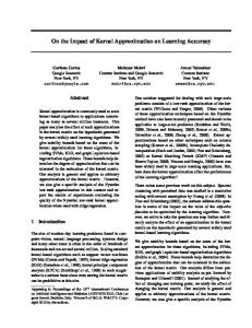
Fig. 1.—Evolution of violent and property crime rates. Adopting are those states that implemented the unilateral reform after the year 1968.

vorce, dummies for abortion accessibility by state and year,27 and dummies for the existence of the death penalty. The comparative evolution between adopting and nonadopting states for raw violent and property crime rates is shown in figure 1. For each of the panels we introduce two vertical lines signaling the years 1970 and 1975, which indicate the period that most states adopted the unilateral divorce law (see table 1). We see, first, that adopting states have a lower incidence of violent crimes than nonadopting states. On the other hand, adopting states have a higher incidence of property crime for the period under analysis. Second, after (and not before) the unilateral reform started there is a monotonic reduction in the gap between adopting and nonadopting states in violent crime rates, with almost no observable difference in the 1990s. However, the gap between adopting and nonadopting states 27 Abortion was legalized nationally in 1973 with Roe v. Wade. Nevertheless, five states (Alaska, California, Hawaii, New York, and Washington) had legalized or quasi-legalized abortion around 1970. Donohue and Levitt (2001) argue that the five states that allowed abortion in 1970 experienced declines in crime rates earlier than the rest of the nation, which legalized in 1973 with Roe v. Wade. However, Joyce (2004) argues that Donohue and Levitt’s evidence that crime fell earlier and faster in the early legalizing states may be spurious, a result of the differential timing in the evolution of crack markets.

This content downloaded from 141.161.91.14 on Tue, 23 Apr 2013 14:10:30 PM All use subject to JSTOR Terms and Conditions

226

This content downloaded from 141.161.91.14 on Tue, 23 Apr 2013 14:10:30 PM All use subject to JSTOR Terms and Conditions

Alabama 1971 Alaska pre-1950 Arizona 1973 Arkansas California 1970 Colorado 1971 Connecticut 1973 Delaware District of Columbia Florida 1971 Georgia 1973 Hawaii 1973 Idaho 1971 Illinois Indiana 1973 Iowa 1970 Kansas 1969 Kentucky 1972 Louisiana Maine 1973 Maryland Massachusetts 1975 Michigan 1972 Minnesota 1974 Mississippi

Unilateral Divorce (1)

No

5 years; later 2 pre-1968

1 year, pre-1968

2 years, 1984

No 1 year, 1977

No

Unilateral Divorce, Including Separation Requirements (2)

Table 1 Divorce Regulations in the United States

1975 1972 1974

1973

1973 1970 1969 1972

1971 1973 1972 1971

1970 1972 1973 1968

1971 1935 1973

1980 pre-1950 pre-1950 1979 pre-1950 1972 1973 pre-1950 1977 1988 1980 1955 pre-1950 1977 1958 pre-1950 pre-1950 1972 1978 1972 1969 1974 1983 1951 pre-1950

Fault 1974 1973 Fault 1970 1971 Fault 1974 Fault 1986 Fault 1960 1990 1977 1973 1972 1990 Fault Fault 1985 Fault Fault Fault 1974 Fault

Unilateral Divorce Equitable Division of No Fault for Property (Gruber 2004) Property and Assets Division and Alimony (3) (4) (5)

227

This content downloaded from 141.161.91.14 on Tue, 23 Apr 2013 14:10:30 PM All use subject to JSTOR Terms and Conditions

1977 1977

1973

1974

1985

1976

†

1953* 1973

1971

1973

1975 1972 1973 1971

2 years; later 1, pre-1968 1-year voluntary s.r., 1977‡

3 years, pre-1968 6 months, pre-1968 2 years, pre-1968

No

3 years; later 1, 1969

3 years, 1980

1 year, 1974

No 1 year, pre-1968

18 months, 1971

2 years, 1973

1978 1977

1973

1970 1987

1985

1975

1953 1971

1971

1933

1973 1972 1967 1971

1974 1976 1972 pre-1950 1988 1971 pre-1950 1962 1981 pre-1950 1990 1975 1971 1979 1979 1979 pre-1950 1959 pre-1950 pre-1950 pre-1950 1982 pre-1950 1984 1978 pre-1950

Fault 1975 1972 1973 Fault 1980 1976 Fault Fault Fault Fault 1975 1971 Fault Fault Fault Fault Fault Fault 1987 Fault Fault 1973 Fault 1977 Fault

Sources.—Columns 1 and 2 are from Friedberg (1998); col. 3 is from Gruber (2004): col. 4 is from Rasul (2004); col. 5 is from Ellman and Rohr (1998). * Date of the law is from Gruber (2004). † Not considered unilateral by Friedberg (1998), although she acknowledges ambiguity. ‡ In this Wisconsin cell, “s.r.” denotes separation requirements.

Missouri Montana Nebraska Nevada New Hampshire New Jersey New Mexico New York North Carolina North Dakota Ohio Oklahoma Oregon Pennsylvania Rhode Island South Carolina South Dakota Tennessee Texas Utah Vermont Virginia Washington West Virginia Wisconsin Wyoming

228

Ca´ceres-Delpiano/Giolito

in terms of property crime rates seems stable during the period, with a marginal tendency to increase after 1985. IV. Results A. Standard and Dynamic Specifications Table 2 presents estimates of the impact of the reform in equation (1), with the natural log of total crime, property crime, and violent crime rates as dependent variables. Each column corresponds to a different specification, with the latter columns controlling for an increasing number of covariates. The first column presents the basic model, including just dummies by year and state as explanatory variables. The second column includes demographic variables; in column 3 we add state aggregate variables, in column 4 policy variables, and in column 5 a linear trend whose impact varies by state.28 Additionally, the estimates for each specification and crime rate have been obtained by using three different codings of the unilateral reform, which are presented in horizontal panels: Friedberg without separation requirement (panel A), Friedberg with separation requirements (panel B), and Gruber (panel C).29 The results in table 2 are robust across specifications and codings used for unilateral divorce. For all specifications, we find that unilateral divorce is associated with an increase in the average violent crime rate for the period under analysis. Nevertheless, the results for property and total crime rates (which is strongly related to property crime) depend on the specification and coding used, with an impact that is marginally negative or/and statistically insignificant. Using Friedberg’s code (panel A), the magnitude of the impact on violent crime is approximately 9% for the complete period (38 violent crimes per 100,000 people), which is stable across specifications. Using alternative codes for unilateral, we obtain similar conclusions and magnitudes. Table 3 presents estimates of gc for the dynamic specification described in equation (2), with the natural log of violent crime as a dependent variable. As before, each column corresponds to a different specification, with the latter columns controlling for an increasing number of covariates. The results in table 3 reveal that the unilateral reform’s impact unfolds during the 8–20 years after the change. Nevertheless, beyond that window the impact depends on the specification used.30 We check the robustness of the results by analyzing the timing of the 28 By including a state-specific time trend, we try to prevent the estimated impact of the unilateral reform from capturing preexisting trends in the selected outcomes. 29 The details of these three codings are in cols. 1, 2, and 3 of table 1, respectively. 30 In online appendix A (table A2), we break violent crime down into its respective subdefinitions. We find that the impact on violent crime is driven mainly by aggravated assaults crimes.

This content downloaded from 141.161.91.14 on Tue, 23 Apr 2013 14:10:30 PM All use subject to JSTOR Terms and Conditions

The Impact of Unilateral Divorce on Crime

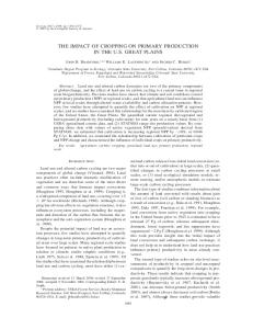
229

change. A causal interpretation of the previous findings would be weakened if we found that crime rates were falling or increasing in adopting states prior to the enactment of unilateral divorce as compared with nonadopting states. In order to examine these issues, we add a series of leads to equation (2), coding dummies for whether the unilateral divorce law would be passed in 1 year, 2 years, and so on. Figure 2 shows the results for this modified specification for the three outcomes in table 2 and for aggravated assault. A vertical line indicates the year that unilateral reform was passed. First, for the four crime rates, in no case are the coefficients of the dummies indicating the periods prior to the divorce law reform (individually or jointly) statistically distinguishable from zero. Second, looking at the coefficients to the left of the vertical line (before the reform), we find no indication of a preexisting trend in adopting states. Third, we obtain the same pattern if we include the rest of the covariates used in the analysis, which suggests that our findings are not driven by other covariates included in the model.31 In table 4, we report the estimates of models (1) and (2) for total violent arrest rates (cols. 1–3), for aggravated assault arrest rates (cols. 4–6), and for murder arrest rates (cols. 7–9). For each type of crime, we split the samples between the white and black subsamples.32 The fact that arrest data are also disaggregated by race is useful for studying whether or not our results are driven by a particular group from the population.33 The first point to note is that, consistent with the 9% increase in the total violent crime rate, unilateral reform is associated as well with an increase of approximately 18% in the total violent arrest rate. In addition, the dynamic specification (2) reveals that the impact of the reform takes place during the first 20 years after the introduction of the reform but that it is statistically insignificant in the long term. For aggregate aggravated assault and murder arrest rates a similar conclusion is obtained: unilateral divorce had a positive impact that unfolds during the first years after the reform. Splitting the samples by race, we observe that the pattern as well as the magnitude of the reform is similar for the race groups. Nevertheless, for murder arrest rates we observe a marginally stronger impact for blacks.34

31 See the previous working paper version of this article (Ca´ceres-Delpiano and Giolito (2008b). 32 However, this level of disaggregation is only available by age or race. That is, we are unable to identify rates at age-race cell level. 33 From now on, we use elasticities evaluated at the sample mean instead of using logs due to the high number of zeros in disaggregated arrest rates. 34 In online appendix A (tables A3 and A4), we present the robustness check for aggravated assault and murder arrest rates to different specifications.

This content downloaded from 141.161.91.14 on Tue, 23 Apr 2013 14:10:30 PM All use subject to JSTOR Terms and Conditions

230

This content downloaded from 141.161.91.14 on Tue, 23 Apr 2013 14:10:30 PM All use subject to JSTOR Terms and Conditions

Violent crime rate

Property crime rate

B. Friedberg (1998), including separation requirements): Total crime rate

Violent crime rate [425 per 100,000 inhabitants]

Property crime rate [4,115 per 100,000 inhabitants]

A. Friedberg (1998) coding: Total crime rate [4,540 per 100,000 inhabitants]

⫺.0713* (.0419) ⫺.0826* (.0459) .0647 (.0454)

⫺.0555 (.0422) ⫺.0637 (.0456) .0964* (.0486)

(1) p Basic

⫺.0528* (.0306) ⫺.0628* (.0329) .058 (.0353)

⫺.0554* (.0324) ⫺.0648* (.0340) .0793* (.0415)

(2) p (1) ⫹ Demographic

Table 2 Average Impact of Unilateral Divorce on Selected Crime Rates (Percent Change)

⫺.0445 (.0296) ⫺.0546* (.0315) .0663* (.0346)

⫺.0427 (.0323) ⫺.0521 (.0336) .0880** (.0405)

(3) p (2) ⫹ State Aggregate

⫺.0439 (.0295) ⫺.0546* (.0312) .0727* (.0378)

⫺.0383 (.0341) ⫺.0481 (.0354) .0959** (.0454)

(4) p (3) ⫹ Policy

.0345 (.0224) .0307 (.0227) .0659* (.0343)

.0451 (.0280) .0401 (.0273) .0941** (.0438)

(5) p (4) ⫹ Trend

231

This content downloaded from 141.161.91.14 on Tue, 23 Apr 2013 14:10:30 PM All use subject to JSTOR Terms and Conditions

⫺.0487 (.0418) ⫺.055 (.0451) .0911* (.0495) 1,632

⫺.051 (.0319) ⫺.0586* (.0335) .0726* (.0419) 1,632

⫺.0436 (.0313) ⫺.0512 (.0326) .0794* (.0410) 1,613

⫺.0407 (.0328) ⫺.0485 (.0342) .0854* (.0435) 1,613

.0442* (.0250) .0405 (.0246) .0835** (.0396) 1,613

Note.—All specifications include dummies by state of residence and dummies by year. Demographic variables include dummies for the fraction of blacks, fraction of immigrants, a quadratic polynomial in state population, and dummies for the state-year age structure of the population. State aggregate variables include the log of state per capita income, the state unemployment rate, and dummies for the consideration of fault for property division and for the existence of norms regarding the equitable division of property in the case of divorce. Other variables include dummies for the existence of death penalty, abortion accessibility, and the lagged incarcerated population and a dummy for the crack introduction in the late 1980s. Sample means appear in brackets in the stub column. Robust standard errors clustered by state are in parentheses. * p ! .10. ** p ! .05.

Observations

Violent crime rate

Property crime rate

C. Gruber (2004): Total crime rate

This content downloaded from 141.161.91.14 on Tue, 23 Apr 2013 14:10:30 PM All use subject to JSTOR Terms and Conditions

.0629 (.0462) .1088* (.0589) .1193* (.0619) .1189* (.0668) .0932 (.0681) .0942 (.0698) .1363 (.0880) 1,632 X X

.0646 (.0390) .0905 (.0564) .0994* (.0563) .1175* (.0636) .0863 (.0704) .0722 (.0738) .0791 (.0884) 1,632 X X X

(2) p (1) ⫹ Demographic .0740* (.0397) .0921 (.0555) .1085* (.0551) .1388** (.0604) .1119 (.0680) .0966 (.0728) .105 (.0859) 1,613 X X X X

(3) p (2) ⫹ State Aggregate .0809* (.0453) .099 (.0592) .1118* (.0557) .1415** (.0594) .1145* (.0668) .1001 (.0720) .1132 (.0868) 1,613 X X X X X

(4) p (3) ⫹ Policy

.0628 (.0445) .0951 (.0577) .1040* (.0576) .1211* (.0617) .0997 (.0682) .0648 (.0705) .065 (.0858) 1,613 X X X X X

(5) p (4) ⫹ Gruber

Note.—All specifications include dummies by state of residence and dummies by year. Demographic variables include dummies for the fraction of blacks, fraction of immigrants, a quadratic polynomial in state population, and dummies for the state-year age structure of the population. State aggregate variables include the log of state per capita income, the state unemployment rate, and dummies for the consideration of fault for property division and for the existence of norms regarding the equitable division of property in the case of divorce. Other variables include dummies for the existence of death penalty, abortion accessibility, and the lagged incarcerated population and a dummy for the crack introduction in the late 1980s. Robust standard errors, clustered by state, are in parentheses. * p ! .10. ** p ! .05.

Observations (1965–96) State fixed effects Year fixed effects State demographic variables State aggregate variables State policy variables

23 years or more since adoption

20–22 years since adoption

16–20 years since adoption

12–15 years since adoption

8–11 years since adoption

4–7 years since adoption

First 3 years after the reform

(1) p Basic

Table 3 Dynamic Impact of Unilateral Divorce on Violent Crime Rates (Rate of Change)

The Impact of Unilateral Divorce on Crime

233

Fig. 2.—Impact of unilateral divorce on selected crime rates: A, violent crime; B, aggravated assault; C, property crime; D, total crime. Each panel reports the point estimates for different regressions. Estimated coefficients refer to dummy variables for a given state k periods before (after) the reform. The omitted category is the dummy for states 3 or 4 years before unilateral divorce is introduced. Nonadopting states and adopting states 8 or more years before the reform are grouped in the same category.

B. Alternative Specification: Age at the Time of the Reform In this section, we make use of the fact that arrest data can be disaggregated by age to analyze potential cohort heterogeneity in the impact of the reform. We concentrate on age-specific arrest rates for the population aged 15–24 since the Uniform Crime Reports record arrests by single year of age for this group only. Tables 5 and 6 present the estimates for violent crime and aggravated assault arrest rates, respectively, which are robust to several specifications. In both tables, column 4 shows the results for the estimation of the equation (3), controlling for confounding factors that vary at the state-year, state-age, or year-age level. The results reveal that in all cases the cohorts affected were those born before the unilateral reform was passed. In fact, for those cohorts born 6 or more years after the reform, the coefficients are not only insignificant but are also considerably smaller than for the rest of the age groups. Finally, we observe that people who were between 8 and 15 years old when the legislation was passed are those who show the largest point estimate for almost all specifications and outcomes. That is, even though

This content downloaded from 141.161.91.14 on Tue, 23 Apr 2013 14:10:30 PM All use subject to JSTOR Terms and Conditions

This content downloaded from 141.161.91.14 on Tue, 23 Apr 2013 14:10:30 PM All use subject to JSTOR Terms and Conditions

.1848*** (.065)

.0766 (.080) .1376* (.074) .2593** (.101) .2677** (.106) .195 (.118) .2277 (.144) .1436 (.159) .2887*** (.073)

.1692** (.068) .2403*** (.086) .3543*** (.116) .3728*** (.125) .3755*** (.127) .4181*** (.142) .2255 (.154)

White (2)

Violent Crime

.2326*** (.082)

.1498** (.074) .1860** (.087) .2770* (.140) .2408** (.116) .1966 (.123) .2208* (.115) .1098 (.135)

Black (3)

.2483*** (.080)

.0981 (.076) .2112** (.099) .3640*** (.120) .3522*** (.126) .3410** (.135) .3789** (.158) .2703 (.177) .3193*** (.101)

.1437* (.086) .2707** (.113) .4394*** (.142) .4544** (.170) .5064*** (.178) .5634*** (.194) .3608* (.198)

White (5)

.2620** (.109)

.1650* (.086) .2178* (.120) .3551* (.188) .2884* (.163) .3330** (.160) .3339** (.160) .2205 (.171)

Black (6)

Aggravated Assault Total (4)

.2354** (.097)

.1121 (.106) .2024** (.091) .3400** (.128) .4356** (.171) .2412 (.220) .2193 (.229) .1972 (.228)

Total (7)

.2663*** (.089)

.1903** (.089) .2688** (.104) .2440* (.139) .3201** (.135) .1939 (.127) .2264 (.137) .0829 (.146)

White (8)

Murder

.3100** (.132)

.3029** (.120) .1717 (.123) .3238** (.131) .4734** (.210) .3362 (.272) .3352 (.286) .0769 (.273)

Black (9)

Note.—N p number of observations p 1,664. Dependent variable is crime rate by age per 100,000 people of the age group in a given state and year. Coefficients represent the rate of change in crime rates for the different cohorts affected by the reform. This elasticity is calculated using the sample mean as the base. All specifications include dummies by state of residence and dummies by year, dummies for the fraction of blacks, fraction of immigrants, dummies for the state-year age structure of the population, a quadratic polynomial in state population, the log of state per capita income, the state unemployment rate, dummies for the consideration of fault for property division and for the existence of norms regarding the equitable division of property in the case of divorce, dummies for the existence of death penalty, abortion accessibility, the lagged incarcerated population and a dummy for the crack introduction in the late 1980s. Robust standard errors, clustered by state, are in parentheses. * p ! .10. ** p ! .05. *** p ! .01.

Average impact of unilateral divorce (1965–97)

23 years or more since adoption

20–22 years since adoption

16–20 years since adoption

12–15 years since adoption

8–11 years since adoption

4–7 years since adoption

First 3 years after the reform

Total (1)

Table 4 Effect of Unilateral Divorce on Arrest Rates by Race (Rate of Change)

The Impact of Unilateral Divorce on Crime

235

some specifications show a significant effect for people who were 16 years old or older, the coefficients are in all cases smaller than the estimates for those who were children between 8 and 15 years old at the time of the reform. C. Stock of People in Institutions: US Census, 1960–2000 In this section, we use a sample of men who were between 15 and 24 years old from the US Census for the period 1960–2000 in order to check the robustness of our previous results. Although census data do not provide information about individual crime history, the information about group quarters helps us to define a proxy variable for the stock of incarcerated people. Therefore, we define as the outcome of interest a dummy variable that takes a value of one if a man lives in an institution, and zero otherwise.35 We define the individual’s exposure to the unilateral reform as well as the state fixed effect in the model by using state of birth. Therefore, in this section we estimate the following variations from equations (2) and (3): inst ibt p ab ⫹ bt ⫹ gXibt ⫹ dZbt ⫹

冘 c

g c Ubtc ⫹ e ibt ,

(4)

and inst ibt p ab ⫹ bt ⫹ gXibt ⫹ dZbt ⫹

冘 c

g cUbtc # 1{aj ≤ [t ⫺ a ⫺ YUnib ] ≤ bj } ⫹ e ibt ,

(5)

where instibt is a dummy variable equal to one if the individual i born in state b lives in an institution at time t, ab and bt represent state of birth and year fixed effects, respectively, Xibt is a vector of individual characteristics, and Zbt denotes time-varying aggregate and policy state variables. Table 7 presents the impact of unilateral reform on the probability of living in an institution. Columns 1–4 present the impact of the reform using different specifications for the complete sample of men. Columns 5 and 6 report the impact for the sample of black men. The upper panel (panel A) presents the dynamic impact of the reform, while the lower panel (panel B) presents the estimates for the specification based on the age at the time of the reform. The results in panel A for the complete sample of men show that the unilateral reform has a positive impact on the likelihood of living in an institution by increasing by 0.21 percentage points the chances of living in an institution during the 5 years after the reform, up to 0.91 percentage points 20–24 years after the reform. These magnitudes in relationship to 35

Unfortunately, after the 1980 US Census it is impossible to distinguish if individuals live in a correctional institution or in another type of facility (mental institution or institutions for the elderly, handicapped, or poor).

This content downloaded from 141.161.91.14 on Tue, 23 Apr 2013 14:10:30 PM All use subject to JSTOR Terms and Conditions

236

This content downloaded from 141.161.91.14 on Tue, 23 Apr 2013 14:10:30 PM All use subject to JSTOR Terms and Conditions

Aged 16 or more when the reform

Aged 12–15 when the reform

Aged 8–11 when the reform

Aged 4–7 when the reform

Aged 0–3 when the reform

Born 1–5 years after the reform

Born 6⫹ years after the reform

(2) p (1) ⫹ Aggregate Variables ⫺.1552 (.162) .012 (.140) .0993 (.102) .1141 (.084) .1381* (.079) .1253* (.063) .0852 (.052)

(1) p Demographic Variables Only ⫺.1946 (.166) ⫺.0223 (.155) .0676 (.111) .0832 (.079) .1109 (.073) .1057* (.062) .0747 (.054)

⫺.0832 (.162) .068 (.138) .1487 (.103) .1577* (.085) .1760** (.079) .1607** (.066) .1229** (.061)

(3) p (2) ⫹ Policy Variables

Table 5 Effect of Unilateral Divorce on Age-Specific Violent Arrest Rates (Rate of Change)

⫺.1365 (.195) ⫺.0511 (.167) .0259 (.113) .0608 (.077) .0988* (.054) .1339*** (.021) .1242*** (.005)

(4) p Interactions

.1682 (.160) .2083* (.108) .3013** (.122) .2287*** (.073) .2208*** (.043) .2841*** (.026) .2376*** (.007)

(5) p Friedberg (1998), Including Separation Requirements

237

This content downloaded from 141.161.91.14 on Tue, 23 Apr 2013 14:10:30 PM All use subject to JSTOR Terms and Conditions

16,640 X X X

16,830 X X

16,640 X X X X X X X

16,830

X X X

16,830

Note.—Dependent variable is violent arrest rate by age per 100,000 people of the age group in a given state and year. Coefficients represent the rate of change in crime rates for the different cohorts affected by the reform. This elasticity is calculated using the sample mean as the base. All specifications include state, year, and age fixed effects. Demographic variables include dummies for the fraction of blacks, fraction of immigrants, a quadratic polynomial in state population, and dummies for the state-year age structure. State aggregate variables include the log of state per capita income, the state unemployment rate, and dummies for the requirement of fault for property division and for the existence of norms regarding the equitable division of property in the case of divorce. Other variables include dummies for the existence of death penalty, abortion accessibility, and early legalizing states and a dummy for the crack introduction in the late 1980s. Robust standard errors, clustered by state, are in parentheses. * p ! .10. ** p ! .05. *** p ! .01.

Observations State demographic variables State aggregate variables State policy variables Age # year interactions State # age interactions State # year interactions

238

This content downloaded from 141.161.91.14 on Tue, 23 Apr 2013 14:10:30 PM All use subject to JSTOR Terms and Conditions

Aged 16 or more when the reform

Aged 12–15 when the reform

Aged 8–11 when the reform

Aged 4–7 when the reform

Aged 0–3 when the reform

Born 1–5 years after the reform

Born 6⫹ years after the reform

(2) p (1) ⫹ Aggregate Variables ⫺.0157 (.160) .2297 (.152) .2990** (.131) .2682*** (.099) .2807*** (.097) .2220** (.086) .1066 (.068)

(1) p Demographic Variables Only ⫺.1148 (.166) .0993 (.178) .1701 (.147) .1589* (.094) .2158** (.089) .1976** (.087) .1075 (.075)

.022 (.167) .2644* (.153) .3338** (.134) .2999*** (.103) .3050*** (.100) .2370** (.092) .1168 (.081)

(3) p (2) ⫹ Policy Variables

⫺.2268 (.340) ⫺.0305 (.302) .12 (.207) .1752 (.122) .2327*** (.072) .2396*** (.026) .2140*** (.007)

(4) p Interactions

Table 6 Effect of Unilateral Divorce on Age-Specific Aggravated Assault Arrest Rates (Rate of Change)

.3254 (.217) .4400** (.174) .5644** (.231) .4450*** (.154) .3699*** (.067) .3521*** (.039) .2745*** (.010)

(5) p Friedberg (1998), Including Separation Requirements

239

This content downloaded from 141.161.91.14 on Tue, 23 Apr 2013 14:10:30 PM All use subject to JSTOR Terms and Conditions

16,640 X X X

16,830 X

X

16,640 X X X X X X X

16,830

X X X

16,830

Note.—Dependent variable is violent arrest rate by age per 100,000 people of the age group in a given state and year. Coefficients represent the rate of change in crime rates for the different cohorts affected by the reform. This elasticity is calculated using the sample mean as the base. All specifications include state, year, and age fixed effects. Demographic variables include dummies for the fraction of blacks, fraction of immigrants, a quadratic polynomial in state population, and dummies for the state-year age structure. State aggregate variables include the log of state per capita income, the state unemployment rate, and dummies for the requirement of fault for property division and for the existence of norms regarding the equitable division of property in the case of divorce. Other variables include dummies for the existence of death penalty, abortion accessibility, and early legalizing states and a dummy for the crack introduction in the late 1980s. Robust standard errors, clustered by state, are in parentheses. * p ! .10. ** p ! .05. *** p ! .01.

Observations State demographic variables State aggregate variables State policy variables Age # year interactions State # age interactions State # year interactions

240

This content downloaded from 141.161.91.14 on Tue, 23 Apr 2013 14:10:30 PM All use subject to JSTOR Terms and Conditions

Average impact of unilateral divorce (1960–2000)

25⫹ years since adoption

20–24 years since adoption

5–19 years since adoption

10–14 years since adoption

5–9 years since adoption

Sample mean A. Dynamic impact of the law: Less than 5 years since adoption .0021* (.001) .0002 (.001) .0034** (.001) .0027 (.002) .0091*** (.003) .0022 (.003) .002 (.001)

.0152

Basic (1)

Black Men

.0031* (.002) .0006 (.001) .0054** (.002) .0032 (.002) .0105*** (.003) .0024 (.002) .0023* (.001)

.0021* (.001) ⫺.0001 (.001) .0034** (.002) .0036** (.002) .0071** (.003) .0026 (.002) .0011 (.001)

⫺.0006 (.002) .0009 (.001) .0015 (.002) .0038 (.002) .0063* (.003) .002 (.002) .0025* (.001)

.0379*** (.008) .0085** (.003) .0377*** (.008) .0219** (.008) .0634*** (.009) .0160* (.009) .0150*** (.005)

.0420 .0454*** (.011) .0079** (.004) .0457*** (.011) .0216** (.009) .0660*** (.010) .0149** (.007) .0150*** (.005)

Friedberg (1998) Including Individual Aggregate Separation Controls Aggregate Controls Requirements Gruber (2004) Only Controls (2) (3) (4) (5) (6)

All Men

Table 7 Effects of Unilateral Divorce on the Probability of Living in an Institution

241

This content downloaded from 141.161.91.14 on Tue, 23 Apr 2013 14:10:30 PM All use subject to JSTOR Terms and Conditions

790,562

.0016 (.002) .0033 (.003) .0045** (.002) .0024* (.001) ⫺.0003 (.001) .0006 (.001) X

.0014 (.002) .0034 (.003) .0051** (.002) .0030** (.001) .0002 (.001) .001 (.001) X X X 790,562

.0016 (.002) .0045* (.002) .0038** (.002) .0017* (.001) ⫺.0005 (.001) ⫺.0001 (.001) X X X 790,562

.0032 (.003) .0015 (.002) .0056** (.002) .0023* (.001) .0011 (.001) .0011 (.001) X X X 790,562 98,283

.0047 (.008) .0272** (.011) .0286*** (.010) .0176*** (.004) .0088* (.005) .005 (.004) X

.0091 (.008) .0167* (.010) .0282** (.011) .0119*** (.004) .0116** (.005) .0155*** (.004) X X X 98,283

Note.—All specifications include state of birth, year, age and race fixed effects, race # year and age # year interactions. State aggregate variables include the log of personal income per capita, the unemployment rate, fractions of blacks, age composition of the population, and dummies for equitable division of property upon divorce and the consideration of fault in property division. Other variables include dummies for the existence of death penalty and abortion accessibility at the year of birth. Robust standard errors, clustered by state of birth, are in parentheses. * p ! .10. ** p ! .05. *** p ! .01.

Individual controls State of residence fixed effects State of residence aggregate variables Observations

Age 15 or more at the change

Age 10–14 at the change

Age 5–9 at the change

Age 0–4 at the change

Born 1–5 years after the change

B. Cohort specific impact of the law: Born 6 or more years after the change

242

Ca´ceres-Delpiano/Giolito

the average sample mean for the period (1.52%) correspond to an increase of approximately 13%–60% in the likelihood of living in an institution. The results in panel A also show that the impact is not lasting after 25 years of the reform except for the sample of black men for whom the impact is considerably stronger. The results in panel B for the complete sample confirm our previous findings. The impact of unilateral reform comes from the individuals who were already born at the time of the reform or born shortly after the change of legislation. V. Impact of the Reform on Related Factors: Mothers, 1960–80 Census In this section, we provide evidence of the impact of unilateral divorce on some of the factors that have been linked to crime (see Sec. II) and for which we have information for the period under consideration. Specifically we analyze the impact on four outcomes characterizing family arrangements and economic outcomes. Our primary data source is the US Census for the period 1960–80. The sample under analysis consists of mothers 25–50 years old with at least one child under age 18 at home.36 The first two variables used in the analysis are associated with marital instability: currently divorced is a dummy variable that takes a value of one if a mother’s marital status is divorced, and zero otherwise; household head is a dummy variable that takes a value of one if the mother is the head of the household and there is not a husband present, and zero otherwise. The third variable in the analysis is real family income (log). Finally, we use the dummy variable poverty that takes a value of one if the mother falls below the poverty line, and zero otherwise. The first specification of interest is as follows: yist p as ⫹ bt ⫹ gXist ⫹ dZst ⫹ vUst⫺1 ⫹ e ist .

(6)

Here yist represents a specific outcome for individual i living in state s at time t; as and ht represent state and year fixed effects. Additionally, Xist is a vector of individual characteristics: age, race, and education of the mother and age of the youngest child. Finally, Zst denotes time-varying aggregate and policy state variables.37 The variable of interest is Ust-1, which is a dummy variable that takes a value of one for those states that had already adopted the unilateral reform the year before the census year. To 36 Recall that we found an impact on crime for people aged 15–24, specifically for the late 1980s and early 1990s. 37 State aggregate variables include the log of personal income per capita, fractions of blacks, age composition of the population, dummies for equitable division of property upon divorce, separation requirements for unilateral divorce, and the consideration of fault in property division.

This content downloaded from 141.161.91.14 on Tue, 23 Apr 2013 14:10:30 PM All use subject to JSTOR Terms and Conditions

The Impact of Unilateral Divorce on Crime

243

Table 8 Effects of Unilateral Divorce on Mother’s Outcomes, US Census 1960–80

Currently divorced % change Household head % change Real family income (log) Below poverty % change Observations

All (1)

High School or Less (2)

At Least Some College (3)

.0091*** (.002) [.0489] 18.61 .0067** (.003) [.0993] 7.15 ⫺.0220* (.013) .0169** (.007) [.3091] 6.02 1,589,456

.0099*** (.002) [.0472] 20.97 .0068** (.003) [.1013] 7.11 ⫺.0232 (.014) .0184** (.008) [.3439] 5.73 1,129,783

.0069*** (.002) [.0556] 12.41 .0043 (.003) [.0916] 5.02 ⫺.0036 (.011) .0043 (.003) [.1741] 2.93 459,673

Note.—Sample means are in brackets. All specifications include state of residence, year, age of the mother, age of the youngest child, race and education fixed effects, age # year and education # year interactions. Other covariates are the log of personal income per capita, the unemployment rate, the age composition of the population, dummies for equitable division of property upon divorce, and the consideration of fault in property division. Robust standard errors, clustered by state of birth, are in parentheses. * p ! .10. ** p ! .05. *** p ! .01.

determine potential heterogeneity in the group of women affected, table 8 shows the results for the whole sample and for two subsamples depending on the education of the mother. In the first row of table 8, we find that unilateral divorce increases the probability of the mother being currently divorced by 18.61%. When we split the sample by education, we observe that the impact is remarkably higher for lower-educated women (a 20.97% increase vs. 12.41% for women with at least some college education). In the second row, we show that unilateral divorce increases the probability that a mother becomes the head of the household by 7.1% both for the whole sample and for women with at most a high school education. Nevertheless, for higher-educated mothers this impact is lower and insignificant. A back-of-the-envelope calculation, using Kelly (2000) elasticity (1.6 for violent crime), suggests that the unilateral reform would imply an 11% increase in violent crime through an increase of the share of single households of low-educated women, which is in line with our findings from previous sections (9%). The results for income also show heterogeneity across mother’s education. Even though the coefficient for family income is only statistically significant at 10%, the results appear to be driven by lower-educated women despite the lack of power of the coefficients. We also find a 6%

This content downloaded from 141.161.91.14 on Tue, 23 Apr 2013 14:10:30 PM All use subject to JSTOR Terms and Conditions

244

Ca´ceres-Delpiano/Giolito

Table 9 Effects of Unilateral Divorce on Mother’s Outcomes by Age of Youngest Child at the Time of the Reform, US Census 1960–80

Born 6⫹ years after the reform Born 1–5 years after the reform Aged 0–4 when the reform Aged 5–9 when the reform Aged 10 or more when the reform Observations

Currently Divorced (1)

Head of Household (2)

Real Family Income (Log) (3)

⫺.0258*** (.008) ⫺.0001 (.004) .0153*** (.003) .0162*** (.003) .0107*** (.002) 1,589,456

⫺.0248*** (.006) ⫺.0013 (.004) .0142*** (.003) .0126*** (.003) .0037 (.003) 1,589,456

.0114 (.015) ⫺.0188 (.013) ⫺.0368*** (.011) ⫺.0245*** (.009) ⫺.0189* (.009) 1,575,182

Below Poverty (4) ⫺.0057 (.009) .0129* (.007) .0206*** (.006) .0224*** (.005) .0242*** (.005) 1,589,456

Note.—All specifications include state of residence, year, age of the mom, age of the youngest child, race and education fixed effects, and age # year, race # year and education year interactions. Other covariates are the log of personal income per capita, the unemployment rate, and age composition of the population. We also include dummies for equitable division of property upon divorce and the consideration of fault in property division. Robust standard errors, clustered by state of residence, are in parentheses. * p ! .10. ** p ! .05. *** p ! .01.

increase in the probability that mothers fall below the poverty line, with this result being entirely driven by the subsample of women with lower education. These findings suggest a negative impact of unilateral divorce on the lower tail of the income distribution, which is consistent with the results in Ananat and Michaels (2008) and therefore in the context of Kelly’s (2000) findings regarding a causal relationship between inequality and violent crime. Finally, to find out which cohorts of children were more affected by the reform, we apply a similar specification to the one in equation (3), in this case to individual census data: yist p as ⫹ bt ⫹ gXist ⫹ dZst ⫹

冘 j

g jUst # {aj ≤ [t ⫺ a ⫺ YUni s ] ≤ bj } ⫹ e ist .

(7)

In this case a represents the age of the woman’s youngest child, and therefore [t ⫺ a] indicates the child’s year of birth. Table 9 displays the results of specification (7) for the four outcomes considered in this section. Observe that, except in the case of poverty, which shows a marginally significant impact for children born 1–5 years after the reform, all other positive impacts are for families whose youngest child was already born at the time of the reform. Notice that, in the case of a divorced or head-of-household mother, we find significant negative

This content downloaded from 141.161.91.14 on Tue, 23 Apr 2013 14:10:30 PM All use subject to JSTOR Terms and Conditions

The Impact of Unilateral Divorce on Crime

245

impacts for children born more than 5 years after the reform. These results suggest that a specific group of mothers, those whose youngest child was born before the unilateral reform was passed, are more likely to be a single household head, to have lower family incomes, and to be below the poverty line. Comparing the last results with those in tables 4–6 (arrest rates) and 7 (institutions-census data), it is easy to see that their youngest children belong to the same cohorts that, years later, become more likely to be arrested or institutionalized. VI. Conclusion In this article, we study the impact of unilateral divorce on crime. Previous research has suggested that divorce laws affected marriage selection and produced some negative effects on individuals who experienced the reform as children. Here we study whether those changes affected crime and arrest rates in states that passed unilateral divorce laws. First, using data from the FBI’s Uniform Crime Report program for the period 1965–96 and differences in the timing in the introduction of the reform, we find that unilateral divorce has a positive impact on violent crime rates, with a 9% average increase for the period under consideration. Applying a similar specification to arrest data confirms our previous results, with an increase of around 18% for violent crime arrest rates. In both cases, a dynamic specification tells us that the impact is mostly concentrated between 8 and 15 years after the reform. Consistent with these results, by using US Census data for 1960–2000 we find that unilateral divorce is associated with an increase in the fraction of institutionalized people. In this case, the geographic source of variation is established at the state of birth level, which gives us another robustness check to our results since our hypothesis is that the mechanism affects the individuals when they are children. We then use the age at the reform as the second source of variation. We are not only able to confirm the positive effect on different types of violent arrests rates, but we also find an impact for property crimes. The results confirm that the impact comes mostly from cohorts who were already born at the time of the reform. Our results on violent crime and aggravated assault are robust to a specification that controls for all confounding factors that may have been operating at the state-year, state-age, or age-year-level. Finally, we provide supporting evidence about some potential mechanisms underlying our results on crime. Using a sample of mothers from the US Census for the period 1960–80, we find that low-educated mothers were more likely to become the head of the household and to fall below the poverty line. Therefore, our results suggest that a potential channel linking the unilateral reform with the increase in crime might have been

This content downloaded from 141.161.91.14 on Tue, 23 Apr 2013 14:10:30 PM All use subject to JSTOR Terms and Conditions

246

Ca´ceres-Delpiano/Giolito

the worsening in economic conditions of mothers and the increase in income inequality as unintended consequences of the reform. References Ananat, Elizabeth, and Guy Michaels. 2008. The effect of marital breakup on the income distribution of women with children. Journal of Human Resources 43, no. 3:611–29. Alesina, Alberto, and Paola Giuliano. 2007. Divorce, fertility and the value of marriage. Unpublished manuscript. Department of Economics, Harvard University. Bedard, Kelly, and Olivier Descheˆnes. 2005. Sex preferences, marital dissolution, and the economic status of women. Journal of Human Resources 40, no. 2:411–34. Bertrand, Marianne, Esther Duflo, and Sendhil Mullainathan. 2004. How much should we trust differences-in-differences estimates? Quarterly Journal of Economics 119, no. 1:249–75. Blau, Judith R., and Peter M. Blau. 1982. The cost of inequality: Metropolitan structure and violent crime. American Sociological Review 47, no. 1:114–29. Ca´ceres-Delpiano, Julio, and Eugenio Giolito. 2008a. How unilateral divorce affects children. Discussion paper no. 3342, Institute for the Study of Labor, Bonn. ———. 2008b. The impact of unilateral divorce on crime. Discussion paper no. 3380, Institute for the Study of Labor, Bonn. Chiappori, Pierre Andre´, Bernard Fortin, and Guy Lacroix. 2002. Marriage markets, divorce legislation, and household labor supply. Journal of Political Economy 85, no. 6:1141–87. Chilton, Roland, and Dee Weber. 2000. Uniform crime reporting program data (United States): Arrests by age, sex, and race for Police Agencies in Metropolitan Statistical Areas, 1960–1997 (Computer file). 2nd ICPSR version. Amherst: University of Massachusetts (producer). Ann Arbor: Inter-university Consortium for Political and Social Research (distributor). Dee, Thomas S. 2003. Until death do you part: The effects of unilateral divorce on spousal homicides. Economic Inquiry 41, no. 1:163–82. Donohue, John J., and Steven Levitt. 2001. The impact of legalized abortion on crime. Quarterly Journal of Economics 116, no. 2:379–420. ———. 2004. Further evidence that legalized abortion lowered crime: A reply to Joyce. Journal of Human Resources 39, no. 1:29–49. ———. 2008. Measurement error, legalized abortion, and the decline in crime: A response to Foote and Goetz. Politics and the Life Sciences 123, no. 1:425–40. Donohue, John J., and Justin Wolfers. 2006. Uses and abuses of empirical

This content downloaded from 141.161.91.14 on Tue, 23 Apr 2013 14:10:30 PM All use subject to JSTOR Terms and Conditions

The Impact of Unilateral Divorce on Crime

247

evidence in the death penalty debate. Stanford Law Review 58:791– 846. Drewianka, Scott. 2004. Divorce law and family formation. Journal of Population Economics 21, no. 2:485–503. Ellman, Ira, and Sharon Lohr. 1998. Dissolving the relationship between divorce laws and divorce rates. International Review of Law and Economics 18, no. 3:341–59. Fajnzylber, Pablo, Daniel Lederman, and Norman Loayza. 2002. Inequality and violent crime. Journal of Law and Economics 45, no. 1: 1323–57. Foote, Christopher, and Christopher Goetz. 2008. The impact of legalized abortion on crime: Comment. Quarterly Journal of Economics 123, no. 1:407–23. Friedberg, Leora. 1998. Did unilateral divorce raise divorce rates? Evidence from panel data. American Economic Review 88, no. 3:608–27. Fryer, Roland, Paul Heaton, Steven Levitt, and Kevin Murphy. 2005. Measuring the impact of crack cocaine. Working paper no. 11318, National Bureau of Economic Research, Cambridge, MA. Gray, Jeffrey S. 1998. Divorce-law changes, household bargaining, and married women’s labor supply. American Economic Review 88, no. 3: 628–42. Gruber, Jonathan. 2004. Is making divorce easier bad for children? Journal of Labor Economics 22, no. 4:799–833. Johnson, John, and Christopher Mazingo. 2000. The economic consequences of unilateral divorce for children. Research Working Paper no. 00-0112, University of Illinois CBA Office of Research. Joyce, Ted. 2004. Did legalized abortion lower crime? Journal of Human Resources 39, no. 1:1–28. ———. 2009. A simple test of abortion and crime. Review of Economics and Statistics 91, no. 1:112–23. Kelly, Morgan. 2000. Inequality and crime. Review of Economics and Statistics 82, no. 4:530–39. Lee, Jin Young, and Gary Solon. 2011. The fragility of estimated effects of unilateral divorce laws on divorce rates. Working Paper no. 16773, National Bureau of Economic Research, Cambridge, MA. Lochner, Lance, and Enrico Moretti. 2004. The effect of education on crime: Evidence from prison inmates, arrests, and self-reports. American Economic Review 94, no. 1:155–89. Matouschek, Niko, and Imran Rasul. 2008. The economics of the marriage contract: Theories and evidence. Journal of Law and Economics 51 (February): 59–110. Matsueda, Ross L, and Karen Heimer. 1987. Race, family structure, and delinquency: A test of differential association and social control theories. American Sociological Review 52, no. 6:826–40.

This content downloaded from 141.161.91.14 on Tue, 23 Apr 2013 14:10:30 PM All use subject to JSTOR Terms and Conditions

248

Ca´ceres-Delpiano/Giolito

Mechoulan, Ste´phane. 2005. Economic theory’s stance on no-fault divorce. Review of the Economics of the Household 3, no. 3:337–59. ———. 2006. Divorce laws and the structure of the American family. Journal of Legal Studies 35, no. 1:143–74. Page, Marianne E., and Ann Huff Stevens. 2004. The economic consequences of absent parents. Journal of Human Resources 39, no. 1:80– 107. Paxson, Christina, and Jane Waldfogel. 2002. Work, welfare, and child maltreatment. Journal of Labor Economics 20, no. 3:435–74. Peters, H. Elizabeth. 1986. Marriage and divorce: Informational constraints and private contracting. American Economic Review 76, no. 3: 437–54. Rand, Alicia. 1987. Transitional life events and desistance from delinquency and crime. In From boy to man, from delinquency to crime, ed. Marvin E. Wolfgang, Terence P. Thornberry, and Robert M. Figlio. Chicago: University of Chicago Press. Rasul, Imran. 2004. The impact of divorce laws on marriage. Unpublished manuscript, Chicago Graduate School of Business, University of Chicago. Ruggles, Steven, J. Trent Alexander, Katie Genadek, Ronald Goeken, Matthew Schroeder, and Matthew Sobek. 2010. Integrated public use microdata series: Version 5.0 (Machine-readable database). Minneapolis: University of Minnesota. Sampson, Robert J. 1987. Urban black violence: The effect of male joblessness and family disruption. American Journal of Sociology 93, no. 2:348–82. Sampson, Robert J., John H. Laub, and Christopher Wimer. 2006. Does marriage reduce crime? A counterfactual approach to within-individual causal effects. Criminology 44, no. 3:465–508. Stevenson, Betsey. 2007. The impact of divorce laws on marriage-specific capital. Journal of Labor Economics 25, no. 1:75–94. ———. 2008. Divorce-law and women’s labor supply. Journal of Empirical Legal Studies 5, no. 4:853–73. Stevenson, Betsey, and Justin Wolfers. 2006. Bargaining in the shadow of the law: Divorce laws and family distress. Quarterly Journal of Economics 121, no. 1:267–88. Wilson, William J. 1987. The truly disadvantaged: The inner city, the underclass, and public policy. Chicago: University of Chicago Press Wolfers, Justin. 2006. Did unilateral divorce raise divorce rates? A reconciliation and new results. American Economic Review 96, no. 5:1802– 20.

This content downloaded from 141.161.91.14 on Tue, 23 Apr 2013 14:10:30 PM All use subject to JSTOR Terms and Conditions