JULY 2005
ZURITA-GOTOR AND CHANG
2261
The Impact of Zonal Propagation and Seeding on the Eddy–Mean Flow Equilibrium of a Zonally Varying Two-Layer Model PABLO ZURITA-GOTOR
AND
EDMUND K. M. CHANG
ITPA/MSRC, State University of New York at Stony Brook, Stony Brook, New York (Manuscript received 31 May 2004, in final form 22 November 2004) ABSTRACT This paper investigates the role of zonal propagation for the equilibration of zonally varying flow. It is hypothesized that there exist two ideal limits, for very small or very large group speed. In the first limit the eddies equilibrate locally with the forcing, while in the second limit the equilibration can only be understood in a global sense. To understand these two limits and to assess which is more relevant for the extratropical troposphere, a series of idealized experiments that involves changing the magnitude of the uniform zonal wind is performed. The results of the idealized model experiments suggest that the actual troposphere is likely to be in a transition regime between the two limits, but perhaps closer to the global than the local limit. Near the global limit, both the eddy amplitude and local baroclinicity over the baroclinic zone are strongly affected by the amount of upstream seeding. When the propagation speed is reduced relative to the control run, the zonal mean eddy activity decreases because the residence time increases more over the stable part of the channel than along the baroclinic zone. With the decrease in upstream seeding, the local supercriticality along the baroclinic zone increases, although the increase is moderate. The decrease in seeding and increase in baroclinicity partially offset the effects of each other, leading to only small changes in the maximum eddy amplitude downstream of the baroclinic zone. Changes in upstream seeding can also be achieved by enhanced damping. When the eddies are locally damped, the baroclinicity is also enhanced downstream of the damping region due to reduced eddy fluxes. For typical parameters, the recovery of the eddy amplitude occurs over very long distances. Based on these idealized results, it is argued that the coexistence of enhanced baroclinicity and weaker eddy amplitude over the Pacific storm track, as compared to the Atlantic storm track, is consistent with the effects of strong eddy damping over Asia.
1. Introduction It has long been known that the thermal structure in the extratropical troposphere is defined by the competition between the diabatic forcing and the dynamical heat fluxes, associated for the most part with equilibrating baroclinic waves (Peixoto and Oort 1992). However, we still lack a simple theory that explains what determines the mean baroclinicity and eddy amplitude in the extratropics, and how the two are related. This is the case not just for the very complex atmospheric system, but even for the highly idealized forced– dissipative baroclinic models often used to conceptualize this system. Naturally, one would expect the eddy amplitude and basic-state adjustment (with respect to some reference eddy-free equilibrium) to be related in such systems.
Corresponding author address: Dr. Pablo Zurita-Gotor, Geophysical Fluid Dynamics Laboratory, Princeton University Forrestal Campus, Rm. 237, U.S. Route 1, Princeton NJ 08542. E-mail:
[email protected]
© 2005 American Meteorological Society
JAS3473
This is made explicit in the potential momentum framework of P. Zurita-Gotor and Lindzen (2005, unpublished manuscript) in which the restoration of the mean and the eddy dissipation locally balance everywhere in statistical equilibrium. However, this forced–dissipative balance offers little predictive value because the local character of the equilibrium only holds for the timemean, but the adjustment is nonlocal in nature. Thus, a fundamental aspect of the equilibration is the propagation of the waves between the source and sink regions of wave activity. The role of meridional eddy propagation for the baroclinic equilibration, particularly in the nonlinear stage, has long been recognized (Simmons and Hoskins 1978). In contrast, the effect of zonal propagation/ downstream development remains little studied. Although it is well established that downstream development is one of the main terms contributing to the growth and decay of individual eddies (Chang 2000), it is unclear whether this has any impact on the wave– mean flow equilibrium. Chang and Orlanski (1993) performed downstream development experiments in an
2262
JOURNAL OF THE ATMOSPHERIC SCIENCES
idealized model, with eddies seeded at an initial longitude and equilibrating downstream. They found a supercritical region just downstream of the forcing, in which the wave–mean flow interaction is limited by the upstream seeding. The question is whether zonal propagation could also be relevant for the equilibrated state of the periodic problem. This is a more complicated question because the seeding is determined internally in that problem.1 The zonal localization of the eddy energy (Lee and Held 1993) is likely to affect the supercriticality of the equilibrated state, if only due to intermittency (Esler and Haynes 1999). The observational study of Chang (2000) also shows that individual eddies often decay through zonal radiation at a time at which the baroclinic conversions are still peaking, which suggests that the wave–mean flow interaction might also be limited by propagation in this case. While the relevance of zonal propagation for the supercriticality of the zonally homogeneous problem is still an open question, there is little doubt that zonal propagation is an important factor in the zonally varying case. When the forcing and/or dissipation vary longitudinally, the extent to which the eddies equilibrate with the local or with the zonal-mean baroclinicity is likely to depend on how fast the eddies propagate downstream. This was first recognized by Pierrehumbert (1984) in his study of the instability of zonally varying flow. Pierrehumbert established a distinction between global and local modes and related them to the concepts of absolute and convective instability. When the group speed is slow, the flow is absolutely unstable and local modes can grow in situ, feeding on the maximum baroclinicity of the flow. However, when the group speed is large, the flow is only convectively unstable and baroclinic growth, in the form of global modes, requires the recycling of the eddy energy. In the two-way equilibration problem, the extent to which the eddy–mean flow equilibrium is determined locally or globally should also depend on zonal propagation. When the group speed is sufficiently slow, we expect the eddies to equilibrate locally at every longitude with the mean flow, at least on scales larger than the Rossby radius. This would imply that the basic-state baroclinicity should be bounded at all longitudes by the equilibrium value of the zonally symmetric problem while, in the absence of upstream seeding, the eddy amplitude should vanish over the stable regions. However, as the group speed increases, the eddies no longer have time to equilibrate locally. In that case, we expect the baroclinicity over the strongly forced regions to be enhanced relative to the symmetric problem with the same level of forcing. The reason is that the seeding at the entrance of these regions would be reduced and
1 For the purpose of this paper, the seeding is defined as the zonal eddy energy flux at the entrance of the baroclinic zone, which is a function of the eddy amplitude and group speed.
VOLUME 62
characteristic of upstream regions with weaker forcing. Reversibly, the eddy amplitudes over the regions with weaker forcing would be larger than expected based solely on that level of forcing as the eddies leak from the more baroclinic regions upstream. In the limit of infinite group speed the eddies should only be sensitive to the zonal mean properties of the flow. Following Pierrehumbert (1984), we refer to these two limits of zero (infinite) group speed as the local (global) equilibration limit. Except in the local limit, we do not expect a one-toone relation between baroclinicity and eddy amplitude, even for the same (local) forcing. An example is provided by the Northern Hemisphere storm tracks: while the baroclinicity is larger in the Pacific, the eddies are stronger along the Atlantic storm track (e.g., Hoskins and Hodges 2002). Lee and Kim (2003) attributed the weakness of the Pacific storm track to the fact that the potential vorticity (PV) gradients are strong over that region. However, while it is plausible that the tight PV gradients in the Pacific could result from local external forcing, it is also true that one would expect a higher baroclinicity in the Pacific precisely because the eddies are weaker. Thus, the larger baroclinicity and weaker eddy amplitude over the Pacific are not mutually inconsistent when one takes into account the different seeding of both storm tracks. Another example of an anticorrelation between baroclinicity and eddy amplitude is provided by the midwinter suppression of eddy activity over the Pacific (Nakamura 1992). One possible explanation is that the seeding of the Pacific storm track is reduced during midwinter, due to the enhancement of the thermal inversion over the Siberian storm track (Orlanski 1998, 2005). An alternative explanation, originally proposed by Nakamura (1992), is that, when the eddies are advected too fast, they become more sensitive to the mean than to the maximum baroclinicity. A hint to which explanation is more appropriate could be found by adding a (westerly) zonal momentum source that made the equilibration more global. If the eddy amplitude is limited by the upstream seeding, this should enhance the eddy amplitude over the Pacific, while it should reduce it if advection is the limiting factor. This paper investigates the relevance of zonal propagation and seeding for the inhomogeneous problem using a simple, zonally varying two-layer model. The model is described in section 2. Section 3 studies the sensitivity of the model equilibrium to zonal propagation, by adding a uniform barotropic component that only advects the eddies. This analysis allows us to address the relevance of the local and global equilibration limits introduced above and to ascertain which is more appropriate in a realistic setting. We also address the question formulated above of whether the eddies are made stronger or weaker with enhanced advection. Section 4 investigates the sensitivity to seeding and shows that locally damping the eddies also results in
JULY 2005
ZURITA-GOTOR AND CHANG
2263
enhanced baroclinicity downstream of the damping region. Section 5 concludes with a summary of the results and a discussion of their atmospheric implications.
2. Methodology We use for this study a standard two-layer quasigeostrophic model forced by Newtonian cooling, as described by the following equations (see, e.g., Holton 1992): ⭸qn 共⫺1兲n 1 ⫺ 2 ⫺ R ⫽ ⫺J共n, qn ⫹ y兲 ⫺ ⭸t n2 ⫺
1 ␦ ⵜ2n ⫺ ⵜ6n, M n2
共1兲
where qn ⫽ ⵜ2n ⫹ (⫺1)n(1 ⫺ 2)/2n stands for the potential vorticity in the upper (n ⫽ 1) and lower (n ⫽ 2) layers, and n is the corresponding streamfunction. The Rossby deformation radius based on the layer depth is n ⫽ 700 km, which we take to be equal in both layers. There is Ekman damping with time scale M ⫽ 4 days in the lower layer, and fourth-order hyperdiffusion is also included to eliminate the small scales. Only the baroclinic part of the flow is forced, with time scale ⫽ 20 days, to a radiative equilibrium profile ⌰R with associated thermal wind: ⭸R ⫽ 关1 ⫹ ␣ sin共2xⲐL兲兴Umax exp共⫺y2Ⲑ2兲. ⫺ ⭸y
共2兲
For the control run, the radiative equilibrium jet has Umax ⫽ 30 m s⫺1 and ⫽ 2200 km. This distance is much smaller than that to the meridional walls (11 ⫻ 103 km), where standard boundary conditions are formulated (g ⫽ a ⫽ 0). We take a typical midlatitude  ⫽ 1.6 ⫻ 10⫺11 m⫺1 s⫺1 and the channel length is 32 ⫻ 103 km. A zonal wavenumber-1 forcing with the same meridional structure as the symmetric part is taken to be the asymmetric part of the forcing. The strength of the asymmetric forcing is controlled by the amplitude parameter ␣. This forcing is different from that used by Whitaker and Dole (1995), who also included a term E with the form J(⌿E j , qj ) in both layers so as to maintain their prescribed stationary wave against the mean flow advection. We opt instead for the form of forcing of Eq. (2) because it is simpler and does not constrain as strongly the equilibrium solution (even when the equilibrium state qE j projects only on zonal wavenumberone, Whitaker and Dole’s forcing also forces other waves owing to nonlinearity). With the previous form of forcing, a large value of ␣ must be chosen to get a reasonable stationary wave against the mean flow advection; unless otherwise stated, we take ␣ ⫽ 3 in the runs presented below. We believe that this is preferable to using a smaller value of (as in Mole and James 1990), which would damp the
FIG. 1. For the control run ( ⫽ 1.75): (top) upper level flow, (middle) temperature, and (bottom) eddy amplitude. We also show (right) the zonal mean wind at equilibration (solid) and in radiative equilibrium (dashed).
eddies too strongly. Though the equilibrium profile has reversed temperature gradients at some longitudes for ␣ ⬎ 1, this is not a problem because the eddies only feel the mean state and the temperature gradient is never reversed in the actual simulations. Our forcing is roughly equivalent to forcing wave one alone with a faster time scale (we also tried this and obtained similar results). The equilibrium state for the control run is displayed in Fig. 1 in which the zonal mean wind, temperature 1/2 field, upper level flow, and eddy amplitude [⬘2] are shown. Note that the storm track peaks downstream of the baroclinicity maximum, so it would be classified as baroclinic in the terminology of Whitaker and Dole (1995). This is reasonable because we only force directly the baroclinic part of the flow. The zonal contrasts in baroclinicity and eddy amplitude observed in the model are both comparable to typical boreal winter values (Chang and Yu 1999), which is remarkable since the forcing is purely baroclinic. To understand the role of zonal propagation for the equilibrated state, we describe in the next section the results from a series of runs in which the advective component of the flow is artificially changed by adding a uniform component ⌬U. This can be easily done in
2264
JOURNAL OF THE ATMOSPHERIC SCIENCES
the quasigeostrophic framework by simply setting the value of the zonal velocity at the meridional walls to Uwalls ⫽ ⌬U. (The velocity at the walls must be constant due to the boundary conditions, but can be otherwise arbitrarily chosen). Note that when this is taken into account, the frictional forcing of the mean remains unchanged under the addition of a uniform zonal wind ⌬U because Ekman friction only damps vorticity. Additionally, we include in the rhs of Eq. (1) a forcing term ⌬UQCR/x where QCR(x, y; n) is the equilibrium (time mean) potential vorticity of the control run. Because this term approximately balances the advection of the basic state PV by the added zonal wind, the enhanced advection only affects the transients to first order. In this setting the mean-flow problem is Galilean invariant except for the eddy forcing, so it is reasonable to assume that the changes in the equilibrium state as ⌬U is varied are due to changes in the wave–mean flow interaction resulting from the varying eddy group speed. In the following we use as a dimensionless measure of zonal propagation the parameter ⫽ cg/L, where cg is the estimated mean group speed. When ⫽ 1, it takes a wave packet a diabatic time scale to cross the channel, which would be comparable to observations (Chang and Yu 1999), while, when is large, the advective time scale is much shorter than the diabatic time scale. We estimated the group speed in the control run by calculating time-lag correlations of wave packet envelopes, as described in Chang and Yu (1999). The resulting zonal group speed at mid channel for the control run is shown in Fig. 2, together with the zonal wind. Its mean value, cg ⫽ 32.5 m s⫺1, gives a propagation parameter ⫽ 1.75. In the experiments with varying ⌬U, was simply calculated by adding ⌬U to the control run group speed. For later reference, a value of ⌬U ⫽ 5 m s⫺1 results in a change in of 0.27.
FIG. 2. Alongchannel zonal group speed (thick, solid) and upper-level zonal wind (broken) for the control run.
VOLUME 62
3. Wind sensitivity experiments a. Equilibration regimes We have performed a series of runs with varying ⌬U as described above. The range of cg values considered is very large, including easterly and westerly values order O(100 m s⫺1). Though the resulting equilibrium states are unrealistic, this wide range is useful for putting into perspective the results of the control run. Figure 3 shows how the time-mean eddy amplitude (upper panel) and time-mean baroclinicity (lower panel) depend on the propagation parameter. We show the maximum, minimum, and mean values zonally, averaging meridionally at mid channel. Here CR stands for the control run ( ⫽ 1.75), while ZS shows the results for a zonally symmetric model with the same forcing. The robustness of the structures shown was confirmed by comparing an ensemble of integrations with different initial conditions (not shown). We distinguish in this figure six different regimes, as explained below. Table 1 summarizes the characteristics of each regime.
FIG. 3. Wind sensitivity analysis: (top) equilibrium eddy amplitude and (bottom) baroclinicity as a function of the propagation parameter . Maximum, minimum, and mean alongchannel values are plotted. The data points are separated by ⌬ ⫽ 0.27 or ⌬U ⫽ 5 m s⫺1. The meaning of the different regions is explained in the text.
JULY 2005
TABLE 1. Characterization of the different regimes shown in Fig. 3. Regime
Range
Explanation
I IIA
⬎ 2.7 1.2 ⬍ ⬍ 2.7
IIB
0.7 ⬍ ⬍ 1.2
Westerly global limit Transition region: global modes dominate Transition region: global modes stabilized, local modes dominate Local regime: group speed vanishes somewhere along the channel Transition to global limit Easterly global limit
III IV V
2265
ZURITA-GOTOR AND CHANG
⫺0.7 ⬍ ⬍ 0.7 ⫺5 ⬍ ⬍ ⫺0.7 ⬍ ⫺5
from the added wind, subtracted for clarity in the top panel of Fig. 4), the structure of the eddy amplitude is very different in both cases. Near the global limit, significant longitudinal modulation in baroclinicity only results in weak modulation in eddy amplitude. The eddy amplitude maximum in Fig. 4 is also located farther downstream from the region of maximum baroclinicity than in the control run. Finally, the storm track is more meridionally confined, which might be due to the focusing of the wave activity along the storm track axis.
2) LOCAL 1) GLOBAL
REGIMES (REGIMES
I
AND
V)
We speculated in the introduction on the existence of a global equilibration limit for large group speed. This is confirmed by Fig. 3, which shows the different curves asymptoting at a constant value for large positive or negative (marked regimes I and V, though the boundaries of these regions are somewhat arbitrary quantitatively). Despite some asymmetry between the transitions to the westerly (regime I) and easterly (regime V) global regimes, Fig. 3 suggests overall that the global equilibrium is the same in both cases. Figure 4 describes in detail the solution for ⫽ 2.7. Despite the mean flow similarity in Figs. 1 and 4 (apart
FIG. 4. As in Fig. 1 but for ⫽ 2.7.
REGIME (REGIME
III)
The local limit corresponds to the limit of zero group speed. It was argued in the introduction that in that limit absolute instability would equilibrate locally so that the maximum alongchannel baroclinicity should be comparable to that of the zonally symmetric problem. Also, the eddy amplitude should vanish along the stable regions as the upstream seeding is eliminated. Figure 3 shows that, although both conditions are approached, neither one is exactly satisfied: the dip in the maximum baroclinicity still exceeds the value of the symmetric problem and there is a remnant eddy amplitude for all values of . The problem is that the theoretical argument assumes the group speed to be exactly zero, which is an idealization. First, because we expect large variability in the group speed itself, both spectrally and in time, only the average group speed can vanish. Additionally, the flow might prevent the cg ⫽ 0 limit, as Delsole and Farrell (1994) have shown that absolute instability equilibrates by locally accelerating the jet and narrowing the absolutely unstable region. When the group speed is nonzero, there is eddy leakage between the high and low baroclinicity regions and scale separation becomes an issue. Another important factor is that the group speed also exhibits significant zonal modulation along the channel (Fig. 2). As a result, the local limit cannot be represented by any single value of ⌬U but, rather, includes a broad range of values (region III in Fig. 3). Thus, a more appropriate definition of the local limit would be the range of ⌬U for which the group speed vanishes somewhere along the channel. It is because of this alongchannel group speed modulation that the dips in minimum eddy amplitude and maximum baroclinicity occur for a different value of . The former should be associated with vanishing group speed along the least unstable region, and the latter with vanishing group speed along the most unstable one. Note that, because the alongchannel cg structure closely follows that of U, the group speed is always more westerly over the most unstable regions than over the least unstable ones (as a reminder, is defined based on the mean alongchannel group speed).
2266 3) TRANSITION
JOURNAL OF THE ATMOSPHERIC SCIENCES REGIMES (REGIMES
II
AND
VOLUME 62
IV)
Regime III displays interesting structure, including a region with anticorrelated baroclinicity and eddy amplitude. Could this be relevant for the midwinter suppression? The answer is likely not because this regime is only reached through the addition of large easterly winds, ⌬U ⬍ ⫺20 m s⫺1. Although it is not clear that the control run necessarily provides the most realistic scenario, due to differences in the momentum balance in the model and in reality, the easterly lower level winds of regime III appear unrealistic. The control run (CR) is embedded in a transition regime (regime II) between the global and local limits. This transition regime is more complicated than both the local and global limits described above, as several effects can play a role. Concentrating first on what happens over the stable region, we can see that the minimum eddy amplitude always reduces with in regime II. There are two reasons for that: the eddies spend more time over the stable region and the seeding from the upstream baroclinic zone is also reduced. More surprising is the fact that the minimum basic state baroclinicity decreases with the eddy amplitude over this region. This happens because the eddies actually maintain the local baroclinicity over this region (primarily through an eddy-driven meridional circulation), as the temperature gradients are reversed in radiative equilibrium. On the other hand, the response over the baroclinic zone is qualitatively different depending on the value of . When the reduction in is moderate (regime IIA), the maximum eddy amplitude remains fairly stable, while the maximum baroclinicity also remains stable or even increases (this increase is more obvious in other sets of runs; cf. Fig. 6). On the other hand, when is further reduced (regime IIB), the eddy amplitude over the baroclinic zone increases rapidly, and the eddies are also significantly more efficient in reducing the maximum baroclinicity of the flow. The difference between these two regimes appears to be due to the emergence of local modes for ⬍ 1.2. As will be shown below, in regime IIA global modes dominate, implying that the eddies feel the baroclinicity everywhere along the channel and not just over the high baroclinicity region. Hence, there are two competing effects when the group speed is reduced. On the one hand, the eddies can spend more time over the baroclinic zone, which makes them more efficient at depleting the maximum baroclinicity of the basic state. On the other, the eddy residence time over the stable region also increases, which leads to reduced eddy seeding at the entrance of the baroclinic zone. Since the ability of the eddies to reduce the maximum baroclinicity decreases with in regime IIA, the latter effect must dominate. Figure 5 explains why this is the case. The upper panel of this figure shows how the residence time over
FIG. 5. (top) Eddy residence time over the baroclinic zone (solid) and the stable region (dashed). (bottom) Fraction of time that the characteristic wave packet spends over the baroclinic zone.
the baroclinic zone and the stable region change with . Here, the baroclinic zone/stable region is defined as the range of longitudes over which the baroclinicity is larger/smaller than the zonal mean baroclinicity. The residence time along each region is then calculated taking into account changes in both the length of the region and the average group speed over that region, computed using time-lagged regression of wave packet envelopes. Changes in the group speed have the largest impact (not shown). Figure 5 displays a pronounced maximum for both curves, pointing to nearly vanishing group speeds over the corresponding region. However, these maxima are not collocated, confirming the previous statement that the group speed vanishes for a different value of in each region. The key point to note is that in regime II cg is always larger over the baroclinic zone than over the stable region, which implies that the relative change in cg is larger, and the residence time increases faster over the stable region than over the baroclinic zone when is varied. As a result, the fraction of time that a wave packet spends over the baroclinic zone (lower panel of Fig. 5) reduces with in this regime, which is why a larger supercriticality over this region is required for maintaining the eddies. This explains the stabilization of the global modes as is reduced. Note that the fraction of time that a wave packet
JULY 2005
ZURITA-GOTOR AND CHANG
spends over the baroclinic zone continues decreasing in regime IIB, but this has little impact over the baroclinic zone because local modes emerge and upstream seeding only plays a minor role. There is not an obvious distinction between IVA and IVB regimes in the transition to global equilibration from the easterly side ( ⬍ ⫺0.67). This asymmetry is due to the fact that cg is always most westerly over the baroclinic zone, as implied by the relative position of the two peaks in Fig. 5. Consequently, when the group speed is weak and westerly over the baroclinic zone (regime II), cg is even weaker along the stable region. In contrast, when the group speed is weak but easterly over the baroclinic zone (regime IV), stronger easterly group speeds occur elsewhere in the channel. As a result, the fraction of time that the characteristic wave packet spends over the baroclinic zone decreases (increases) with when approaching the local regime III from the westerly (easterly) side. This explains why upstream seeding only plays a role in regime II, while the transition to the global regime is monotonic in regime IV. To conclude this section, we note that we have repeated the previous analysis for a wide range of parameters, changing the shape and strength of the radiative equilibrium jet, the barotropic shear, the amplitude of the stationary wave, and the frictional and diabatic time scales. It was found that the structure described in Fig. 3 is very robust qualitatively, though quantitative differences of course exist. Not surprisingly, an important factor for understanding these differences is how changes in the global momentum balance affect the mean advection level. For example, Fig. 6 shows how the sensitivity curves change when friction is halved. Decreasing friction leads to a higher eddy energy level, but also to an eastward shift of the wind sensitivity curves due to the enhancement in the mean westerlies.
2267
FIG. 6. As in Fig. 3 except that two sets of lines are plotted. The thin lines are for the standard parameters and the thick lines are for a set of runs with halved friction. Note that the x axis is unshifted (unlike in Fig. 3), to emphasize the fact that the mean group speed is different in both cases.
be borne in mind that this only gives the most unstable mode. The results are shown in Fig. 7. As found by many other authors (e.g., Stone and Branscome 1992), the time-mean state is supercritical in our model, though the growth rates are moderate. The significance
b. Linear stability We have shown above that changes in the global advection may have a profound impact on how the zonally varying problem equilibrates. Though part of these changes may be due to nonlinear effects, such as differences in wave breaking arising from changes in deformation (e.g., Whitaker and Dole 1995; Swanson et al. 1997), it appears that the single most important factor explaining the observed changes in wave–mean flow interaction in our runs may simply be changes in the eddy residence time arising from changes in the advection level. Since this only involves the interaction between eddy and mean flow, we investigate in this section to what extent the structure in Fig. 3 can be explained using linear dynamics. With this purpose in mind, we have performed a linear stability analysis of the time-mean state. Since solving the eigenvalue problem is computationally expensive in the zonally varying case, we have opted instead for solving the initial value problem. However, it should
FIG. 7. Linear stability analysis for the full equilibrium state (solid) and for a basic state constructed adding a uniform zonal wind to the control run equilibrium (dashed).
2268
JOURNAL OF THE ATMOSPHERIC SCIENCES
VOLUME 62
FIG. 8. Snapshots of the most unstable mode upper-layer streamfunction for the values of indicated and fixed basic state. The thick line is the 20% envelope contour: (top) a global mode and (bottom) a local mode. (middle) For intermediate values of , the most unstable mode appears to owe its existence to wave accumulation (e.g., Swanson 2000; Mak 2002) rather than to baroclinic instability.
of such small growth rates may be controversial; however, even in linear stochastic models in which by definition all modes are stable, the least damped modes typically dominate the signal (Hall and Sardeshmukh 1998). This suggests that, regardless of whether the turbulent state is self-maintained or stochastically forced, that is, whether it is more appropriate to talk of the most unstable mode or the least damped one, the modal dynamics still plays a role. There are two curves plotted in Fig. 7. The solid line (variable basic state) gives the growth rate of the timemean state observed for a given value of . On the other hand, the dashed line (fixed basic state) was constructed adding a uniform zonal wind component to the time-mean state of the control run. Hence, this latter curve gives differences in growth rate resulting from differences in the zonal advection alone, unlike the solid line, which is also sensitive to the different extent to which the eddies reduce the baroclinicity in the different regimes. The two curves are well correlated in regimes I and II, suggesting that differences in advection are likely responsible for growth rate differences in these regimes (note that this includes the control run). In contrast, the growth rates with fixed and varying basic state are very different in regime III. This is not surprising because it is in this regime that the eddies also modify the mean flow the most (cf. Fig. 3), due to
the large residence times. Note that, although the eddies are generally very efficient at neutralizing absolute instability in regime III, there is a pronounced peak in the growth rate at the transition between regimes IIB and III. The position of that peak is puzzling in that it occurs for a value of for which the group speed vanishes along the stable region rather than over the baroclinic zone (cf. Figure 5; also compare to the peak in maximum eddy amplitude in Fig. 3). A simple explanation might be that it is for this value of that the maximum baroclinicity is largest in regime III. However, there could also be large differences in group speed for the average wave packet of the nonlinear system and the most unstable mode of the time-mean state. Besides being correlated with each other, the curves in Fig. 7 are also consistent in regime II with the nonlinear wind sensitivity displayed in Fig. 3. There is an initial decrease in the global growth rate with decreasing advection in regime IIA, which can again be explained in terms of the relative changes in the residence time along the baroclinic zone and stable region (i.e., the fraction of time that the characteristic wave packet spends over the baroclinic zone decreases with ). However, for ⱕ 1.2 the growth rate in Fig. 7 and the maximum eddy amplitude in Fig. 3 increase rapidly. It was argued above that this was due to the emergence of local modes. This is indeed what Fig. 8 suggests, as the
JULY 2005
ZURITA-GOTOR AND CHANG
structure of the most unstable mode is very different in regimes IIA and IIB. Note that the most unstable mode at the transition between both regimes does not seem to grow through baroclinic instability. To conclude, we note that the dependence of the global growth rate on advection described above is much stronger than in the 2D study of Pierrehumbert (1984) in which the global modes are mostly insensitive to changes in the group speed. We are unaware of any other study that has examined this issue. We believe that the difference with Pierrehumbert’s results is due to the much stronger contrasts in group speed along the channel in our case than in Pierrehumbert’s. In his model, only the baroclinicity is zonally varying, while the barotropic component of the wind is uniform. As a result, the alongchannel differences in group speed should be more moderate than in our case, and the group speed should vanish nearly simultaneously over the stable and unstable zones. This could explain why there is not a clear separation between local and global modes as in our model. Presumably, if the group speed contrast was further enhanced, an intermediate region might exist in which both global and local modes are stabilized (i.e., the group speed would be too large over the baroclinic zone to support absolute instability, and too small over the stable region to allow eddy recycling).
4. The impact of upstream seeding The results of the previous section suggest that it is unlikely that enhanced advection (i.e., increasing ) could lead to a baroclinicity–eddy amplitude anticorrelation of the type found by Nakamura (1992). If anything, eddy amplitude and baroclinicity are positively correlated in regime IIA. When global modes dominate, enhancing the advective component leads to a strengthening rather than a weakening of the eddies because the fraction of time that the characteristic wave packet spends over the baroclinic zone increases. Although an anticorrelation of the type described by Nakamura was found in regimes IIB and III, we believe that these regimes are not realistic. In contrast, seeding might be a more likely candidate to explain the midwinter suppression, as the previous analysis shows that a reduction in seeding might lead to enhanced baroclinicity over the baroclinic zone. The impact of reducing the upstream seeding on the maximum baroclinicity/eddy amplitude is moderate in Fig. 3, but this is only because the reduction in eddy seeding is also accompanied by larger residence times over the main baroclinic zone. The situation would be different if the reduction in eddy seeding was due to stabilization upstream, rather than to global changes in advection as in our runs, which would also be more comparable to the mechanism proposed by Orlanski (1998). To examine this possibility, we have performed a se-
2269
FIG. 9. (top) Eddy amplitude and (bottom) midchannel baroclinicity, normalized by its radiative equilibrium value, for a zonally symmetric run (dashed) and for a run with a permeable sponge with damping time scale s ⫽ 4 days. The sponge region is shown shaded.
ries of runs in which the forcing is homogeneous but the storm track is still longitudinally localized by means of a permeable sponge. This sponge is designed so that the eddies are locally damped without simultaneously restoring the mean baroclinicity (see appendix for details). The sponge damping times are moderate, and enough wave activity still leaks through that absolute instability is not required for the maintenance of the turbulent state. Figure 9 shows the results with a sponge damping time scale of 4 days; the parameters are the same as in the previous runs except that now ␣ ⫽ 0 (i.e., the forcing is zonally symmetric). The upper panel shows the eddy amplitude and the lower panel the midchannel baroclinicity, with the sponge-free solution also plotted broken for comparison. The lower panel shows that, along with the drop in eddy amplitude across the sponge, there is a downstream region with enhanced baroclinicity. Because the sponge region is purposely designed to damp the eddies without restoring the mean (see appendix), this enhanced baroclinicity should be attributed to the weakened eddy fluxes, rather than to direct forcing by the sponge. (Indeed, note that the region with enhanced baroclinicity is observed downstream and outside the sponge). Note that the situation described in Fig. 9 is very
2270
JOURNAL OF THE ATMOSPHERIC SCIENCES
similar to what is observed over the western Pacific. Although differences in the external forcing between the Atlantic and the Pacific cannot be discarded, the simplest explanation as to why the baroclinicity is higher over the Pacific than over the Atlantic is that the eddies are strongly damped over Asia. Figure 9 illustrates the point made in the introduction that high baroclinicity and low eddy amplitude are not necessarily incompatible in the zonally varying problem due to the effects of seeding. Note that the behavior in Fig. 9 is also consistent with the characteristics of the midwinter suppression, as there is both an increase in baroclinicity and a decrease in eddy amplitude. A relevant question is how far downstream the impact of the sponge is felt. We can estimate the e-folding adjustment length as Ladj ⬃ cg/, where cg is the group speed and is a measure of the enhanced supercriticality downstream. Taking a typical group speed of 35 m s⫺1 and a supercriticality of 0.1 day⫺1 (cf. Fig. 7), we obtain Ladj ⫽ 30 ⫻ 103 km, which is roughly consistent with Fig. 9. This simple estimate would suggest that the Pacific storm track fails to reach saturation, which might explain why the Atlantic storm track is stronger.2 Are these numbers realistic? While cg is roughly constrained by the magnitude of the upper level zonal wind, it is not obvious a priori what determines the equilibrium in this problem. In particular, our estimate for was based on the global supercriticality and it is unclear whether the flow can become significantly more supercritical locally than in a global sense. Higher values of would imply smaller adjustment lengths. To get a more reliable estimate of and to ascertain to what extent the supercriticality just downstream of the sponge may exceed its global mean value, we have estimated the local supercriticality as the growth rate of the zonally symmetric problem with the same local properties.3 The results are shown in Fig. 10. As expected, there is enhanced supercriticality just downstream of the sponge location; however, this enhancement is quite moderate. To understand what controls the downstream criticality, it is useful to consider two limits: one with large downstream supercriticality and fast recovery of the eddy amplitude and another with moderate supercriticality and slower eddy recovery. In principle, we would
2 The observational study of Hoskins and Hodges (2002) has shown that cyclones generated in the western Pacific usually dissipate before reaching the Unite States. However, this does not necessarily contradict the hypothesis put forward that the Pacific storm track may fail to reach saturation. The reason is that Hoskins and Hodges only track individual eddies, which may dissipate through downstream development, while coherent wave packets can often be tracked during much longer times (Chang 2000). To be precise, our argument is only concerned with the relative importance of propagation and baroclinic growth (Plumb 1986) and even applies when the group speed is dispersive and the eddy energy propagates in a noncoherent manner. 3 Note that the sponge was not included in this analysis.
VOLUME 62
FIG. 10. Alongchannel supercriticality for the sponge run with s ⫽ 4 days, based on the local flow properties (the sponge is not included in the calculations).
expect this to be dependent on eddy amplitude so that the supercriticality would be enhanced and the recovery would be faster when the eddies are weakened the most. To test this idea, Fig. 11 shows the results from a series of experiments with varying sponge damping. As hypothesized, the baroclinicity just downstream of the sponge increases as the sponge damping is enhanced, though the zonal structure is complex and consists of more than one baroclinic zone. As the flow becomes more supercritical downstream of the sponge, the eddy amplitude also recovers faster. In fact, the upper panel of Fig. 11 shows that dE/dx is relatively insensitive to the sponge damping time scale: dE ⬇ E ⫺ diss ⬇ const, dx cg where E is the eddy kinetic energy and diss the nonlinear eddy dissipation. Hence, the enhancement in and the reduction in E are comparable in our model, which implies that the length required for eddy recovery, O(cg⌬E/E ), is just a function of the eddy amplitude drop ⌬E across the sponge (neglecting the nonlinear dissipation). Thus, stronger eddy damping only leads to longer adjustment lengths, even if the supercriticality increases. Since the eddy amplitude drop in Fig. 9 is moderate compared to observations, our estimate for Ladj is unlikely to overestimate the true atmospheric value, supporting the claim that the Pacific storm track may not reach saturation.
5. Summary and concluding remarks In this work we have investigated the role of zonal advection and eddy dissipation for the equilibration of zonally varying flow. Unlike most previous studies (e.g., Whitaker and Dole 1995), which have primarily con-
JULY 2005
ZURITA-GOTOR AND CHANG
2271
FIG. 11. As in Fig. 9 but for the sponge damping time scales indicated.
centrated on what factors are responsible for the observed modulation of eddy amplitude, we have examined the two-way equilibration problem, including changes in the modulation of the basic state baroclinicity. To understand the effect of zonal eddy propagation, it is useful to consider the idealized limits of zero/ infinite group speed, which we called the local and global limit following Pierrehumbert (1984). Our hypothesis before starting this study, based on diagnostics such as those of Plumb (1986), was that the global limit was more appropriate for the earth’s atmosphere. This was found to be the case in the control run of the simple model; however, the equilibrated state in that run is still sensitive to changes in advection. As the group speed is decreased from the control run, the eddies are somewhat less efficient at transporting heat, leading in some
cases to enhanced baroclinicity over the strongly forced regions. The fact that reducing the group speed may lead to enhanced maximum baroclinicity could be striking at first since the eddies have more time to equilibrate over the more strongly forced regions in that case. We argued that this was due to the effect of reduced upstream seeding, as the group speed is also decreased over the stable regions upstream. Because the group speed is larger over the more unstable regions than over the stable ones, the eddy residence time over the latter is affected the most by a uniform change in group speed. The same mechanism was found to be at work in the linear problem, producing a stabilization of the global modes when the group speed is decreased. This results in a more distinct separation between global and local modes than found in previous studies.
2272
JOURNAL OF THE ATMOSPHERIC SCIENCES
Since our model is only thermally forced, it is not surprising that the model storm tracks would be classified as baroclinic in the terminology of Whitaker and Dole (1995). This explains that the baroclinicity contrasts and changes in eddy residence time play the important role described above. However, the relative role of baroclinic and barotropic processes for the modulation of eddy amplitude along the climatological storm tracks is still an open question (see Chang et al. 2002 for a review). Chang and Orlanski (1993) have shown that it is difficult to produce eddy decay through changes in baroclinicity alone. While pure baroclinic forcing produced realistic longitudinal modulation in our control run, both in baroclinicity and eddy amplitude, it may also be argued that this required an unrealistically strong asymmetric forcing (␣ ⫽ 3). Hence, it is possible that other mechanisms rather than the baroclinicity contrasts, for instance, surface friction and irreversible wave breaking, could be responsible for terminating the storm tracks in the real atmosphere. This was the situation considered in the idealized experiments of section 4, in which the storm tracks were localized by means of enhanced damping over a sponge region. We found that this mechanism was very efficient in producing baroclinicity contrasts, perhaps more so than the asymmetric forcing. Enhanced baroclinicity was observed downstream of the sponge region, due to the weakening of the eddies. We estimated the adjustment length over which the eddies recover, based on the downstream values of group speed and supercriticality. This estimate suggests that the Pacific storm track never reaches saturation. Thus, the enhanced Pacific baroclinicity compared to the Atlantic could simply be explained in terms of the different eddy amplitude at the entrance of both storm tracks. The different eddy energy level along both storm tracks can make the Pacific jet more subtropical and the Atlantic jet more eddy driven (Lee and Kim 2003) even with the same external forcing. Could this mechanism also be relevant for the midwinter suppression? The idealized results of section 3 suggest that, dynamically, seeding is a more plausible candidate than enhanced advection, which does not produce the required baroclinicity–eddy amplitude anticorrelation for realistic wind speeds. Orlanski (1998, 2005) has also provided observational evidence in support of the seeding hypothesis. Though the energy budget analysis of Chang (2001) suggests that diabatic effects play the primary role in the seasonal suppression, other factors are also likely to contribute because some dry models can reproduce part of the suppression signal (Zhang and Held 1999). Moreover, the midwinter anticorrelation is also found in interannual time scales in which diabatic processes do not play a role (Chang 2001). The main difficulty is that no conclusive observational evidence has been found so far of the presumed correlation between the eddy amplitudes over Asia and
VOLUME 62
over the western Pacific (Zhang 1997, and our own unpublished results). This may seem surprising given the strong existing evidence for the seeding of the Pacific storm track by eddy anomalies over Asia (Chang 2005). Thus, the possibility cannot be discarded that the signal is simply very hard to detect, perhaps because the low-frequency storm track variability is dominated by local red noise or because changes in the seeding path associated to the split jet (e.g., Nakamura and Sampe 2002) degrade the correlation. It is noteworthy in this regard that the correlation between the Atlantic and Pacific storm tracks is also very low in the Southern Hemisphere (Chang 2004). An alternative explanation is that the observed anticorrelation between baroclinicity and eddy amplitude on interannual time scales is due to the different meridional structure of the jet. As discussed by Harnik and Chang (2004), stronger jets are typically also narrower, and a broad jet can be more unstable than a more baroclinic but narrower one. Harnik and Chang assumed that the interannual variability of the jet is driven by changes in the external forcing. However, as with baroclinicity, the argument is reversible and it is also true that a narrower jet is expected when the eddies are weakened. Thus, establishing whether it is changes in the external forcing or changes in the upstream seeding that are important for the interannual relation will require a detailed analysis of the forcing of the Pacific jet and its variability, as well as a more careful assessment of the extent to which the Eurasian and Pacific eddy amplitudes are correlated on long time scales. Acknowledgments. We acknowledge financial support by NSF Grant ATM0296076 and NOAA Grant NA16GP2540 and thank the three anonymous reviewers for their comments, which led to a more readable manuscript. The manuscript was partially written while the first author was supported by the Visiting Scientist Program at the NOAA/Geophysical Fluid Dynamics Laboratory, administered by the University Corporation for Atmospheric Research.
APPENDIX A Permeable Sponge In section 3 we describe some simulations using a permeable sponge. The function of this sponge is to selectively reduce, but not eliminate, the eddy amplitude. We damp potential vorticity in this region, using a variable time scale s(x) that is defined by its maximum value but converges smoothly to the undamped solution outside. Since the eddies are not fully eliminated, the equilibrated state over the sponge region should also differ from the radiative equilibrium solution. The most straightforward solution is to simply relax the PV field over the sponge region to its radiative equilibrium profile, with time scale s. However, this
JULY 2005
ZURITA-GOTOR AND CHANG
implies that changes in the sponge damping times affect both the eddy damping and the restoring of the basic state, which makes the interpretation ambiguous. To avoid this ambiguity, we have chosen instead to relax PV to its instantaneous mean along the sponge. This reduces the wiggles in the PV contours without changing their mean position significantly. We found that, while the equilibrium state is quite sensitive to which sponge is used, the results are more naturally interpreted in terms of changes in the eddy damping with this second solution. REFERENCES Chang, E. K. M., 2000: Wave packets and lifecycles of troughs in the upper troposphere: Examples from the Southern Hemisphere summer season of 1984/85. Mon. Wea. Rev., 128, 25– 50. ——, 2001: GCM and observational diagnoses of the seasonal and interannual variations of the Pacific storm track during the cool season. J. Atmos. Sci., 58, 1784–1800. ——, 2004: Are the Northern Hemisphere winter storm tracks significantly correlated? J. Climate, 17, 4230–4244. ——, 2005: The impact of wave packets propagating across Asia on Pacific cyclone development. Mon. Wea. Rev., 133, 1998– 2015. ——, and I. Orlanski, 1993: On the dynamics of a storm track. J. Atmos. Sci., 50, 999–1015. ——, and D. B. Yu, 1999: Characteristics of wave packets in the upper troposphere. Part I: Northern Hemisphere winter. J. Atmos. Sci., 56, 1708–1728. ——, S. Lee, and K. Swanson, 2002: Storm track dynamics. J. Climate, 15, 2163–2183. Delsole, T., and B. Farrell, 1994: Nonlinear equilibration of localized instabilities on a baroclinic jet. J. Atmos. Sci., 51, 2270– 2284. Esler, J. G., and P. H. Haynes, 1999: Mechanisms for wave packet formation and maintenance in a quasigeostrophic two-layer model. J. Atmos. Sci., 56, 2457–2490. Hall, N. M. J., and P. D. Sardeshmukh, 1998: Is the time-mean Northern Hemisphere flow baroclinically unstable? J. Atmos. Sci., 55, 41–56. Harnik, N., and E. K. M. Chang, 2004: The effects of variations in jet width on the growth of baroclinic waves: Implications for
2273
midwinter Pacific storm track variability. J. Atmos. Sci., 61, 23–40. Holton, J., 1992: An Introduction to Dynamic Meteorology. 3d ed. Academic Press, 511 pp. Hoskins, B. J., and K. I. Hodges, 2002: New perspectives on the Northern Hemisphere winter storm tracks. J. Atmos. Sci., 59, 1041–1061. Lee, S., and I. M. Held, 1993: Baroclinic wave packets in models and observations. J. Atmos. Sci., 50, 1413–1428. ——, and H.-K. Kim, 2003: The dynamical relation between subtropical and eddy-driven jets. J. Atmos. Sci., 60, 1490–1503. Mak, M., 2002: Wave-packet resonance: Instability of a localized barotropic jet. J. Atmos. Sci., 59, 823–836. Mole, N., and I. N. James, 1990: Baroclinic adjustment in zonally varying flows. Quart. J. Roy. Meteor. Soc., 116, 247–268. Nakamura, H., 1992: Midwinter suppression of baroclinic wave activity in the Pacific. J. Atmos. Sci., 49, 1629–1642. ——, and T. Sampe, 2002: Trapping of synoptic scale disturbances into the North-Pacific subtropical jet core in midwinter. Geophys. Res. Lett., 29, 1761, doi:10.1029/2002GL015535. Orlanski, I., 1998: Poleward deflection of storm tracks. J. Atmos. Sci., 55, 2577–2602. ——, 2005: A new look at the Pacific storm track variability: Sensitivity to tropical SSTs and to upstream seeding. J. Atmos. Sci., 62, 1367–1390. Peixoto, J. P., and A. H. Oort, 1992: Physics of Climate. AIP Press, 520 pp. Pierrehumbert, R. T., 1984: Local and global instability of zonally varying flow. J. Atmos. Sci., 41, 2141–2162. Plumb, R. A., 1986: Three-dimensional propagation of transient quasi-geostrophic eddies and its relationship with the eddy forcing of the time-mean flow. J. Atmos. Sci., 43, 1657–1678. Simmons, A. J., and B. J. Hoskins, 1978: The lifecycles of some nonlinear baroclinic waves. J. Atmos. Sci., 35, 414–432. Stone, P. H., and L. Branscome, 1992: Diabatically forced, nearly inviscid eddy regimes. J. Atmos. Sci., 49, 355–367. Swanson, K. L., 2000: Stationary wave accumulation and the generation of low-frequency variability in zonally varying flows. J. Atmos. Sci., 57, 2262–2280. ——, P. J. Kushner, and I. M. Held, 1997: Dynamics of barotropic storm tracks. J. Atmos. Sci., 54, 791–810. Whitaker, J. S., and R. M. Dole, 1995: Organization of storm tracks in zonally varying flows. J. Atmos. Sci., 52, 1178–1191. Zhang, Y., 1997: On the mechanisms of the mid-winter suppression of the Pacific stormtrack. Ph.D. thesis, Princeton University, 152 pp. ——, and I. M. Held, 1999: A linear stochastic model of a GCM’s midlatitude storm tracks. J. Atmos. Sci., 56, 3416–3435.