The Annals of Statistics 2013, Vol. 41, No. 2, 693–721 DOI: 10.1214/13-AOS1101 © Institute of Mathematical Statistics, 2013
THE MULTI-ARMED BANDIT PROBLEM WITH COVARIATES B Y V IANNEY P ERCHET1
AND
P HILIPPE R IGOLLET2
Université Paris Diderot and Princeton University We consider a multi-armed bandit problem in a setting where each arm produces a noisy reward realization which depends on an observable random covariate. As opposed to the traditional static multi-armed bandit problem, this setting allows for dynamically changing rewards that better describe applications where side information is available. We adopt a nonparametric model where the expected rewards are smooth functions of the covariate and where the hardness of the problem is captured by a margin parameter. To maximize the expected cumulative reward, we introduce a policy called Adaptively Binned Successive Elimination (ABSE) that adaptively decomposes the global problem into suitably “localized” static bandit problems. This policy constructs an adaptive partition using a variant of the Successive Elimination (SE) policy. Our results include sharper regret bounds for the SE policy in a static bandit problem and minimax optimal regret bounds for the ABSE policy in the dynamic problem.
1. Introduction. The seminal paper [19] introduced an important class of sequential optimization problems, otherwise known as multi-armed bandits. These models have since been used extensively in such fields as statistics, operations research, engineering, computer science and economics. The traditional multi-armed bandit problem can be described as follows. Consider K ≥ 2 statistical populations (arms), where at each point in time it is possible to sample from (pull) only one of them and receive a random reward dictated by the properties of the sampled population. The objective is to devise a sampling policy that maximizes expected cumulative rewards over a finite time horizon. The difference between the performance of a given sampling policy and that of an oracle, that repeatedly samples from the population with the highest mean reward, is called the regret. Thus, one can re-phrase the objective as minimizing the regret. When the populations being sampled are homogeneous, that is, when the sequential rewards are independent and identically distributed (i.i.d.) in each arm, the family of upper-confidence-bound (UCB) policies, introduced in [14], incur a regret of order log n, where n is the length of the time horizon, and no other Received June 2012; revised January 2013.
1 Supported in part by the ANR Grant ANR-10-BLAN-0112.
2 Supported in part by the NSF Grants DMS-09-06424, DMS-10-53987.
MSC2010 subject classifications. Primary 62G08; secondary 62L12. Key words and phrases. Nonparametric bandit, contextual bandit, multi-armed bandit, adaptive partition, successive elimination, sequential allocation, regret bounds.
693
694
V. PERCHET AND P. RIGOLLET
“good” policy can (asymptotically) achieve a smaller regret; see also [4]. The elegance of the theory and sharp results developed in [14] hinge to a large extent on the assumption of homogenous populations and hence identically distributed rewards. This, however, is clearly too restrictive for many applications of interest. Often, the decision maker observes further information and based on that, a more customized allocation can be made. In such settings, rewards may still be assumed to be independent, but no longer identically distributed in each arm. A particular way to encode this is to allow for an exogenous variable (a covariate) that affects the rewards generated by each arm at each point in time when this arm is pulled. Such a formulation was first introduced in [24] under parametric assumptions and in a somewhat restricted setting; see [9, 10] and [23] for very different recent approaches to the study of such bandit problems, as well as references therein for further links to antecedent literature. The first work to venture outside the realm of parametric modeling assumptions appeared in [25]. In particular, the mean response in each arm, conditionally on the covariate value, was assumed to follow a general functional form; hence one can view their setting as a nonparametric bandit problem. They propose a variant of the ε-greedy policy (see, e.g., [4]) and show that the average regret tends to zero as the time horizon n grows to infinity. However, it is unclear whether this policy satisfies a more refined notion of optimality, insofar as the magnitude of the regret is concerned, as is the case for UCB-type policies in traditional bandit problems. Such questions were partially addressed in [18] where near-optimal bounds on the regret are proved in the case of a two-armed bandit problem under only two assumptions on the underlying functional form that governs the arms’ responses. The first is a mild smoothness condition, and the second is a so-called margin condition that involves a margin parameter which encodes the “separation” between the functions that describe the arms’ responses. The purpose of the present paper is to extend the setup of [18] to the K-armed bandit problem with covariates when K may be large. This involves a customized definition of the margin assumption. Moreover, the bounds proved in [18] suffered two deficiencies. First, they hold only for a limited range of values of the margin parameter and second, the upper bounds and the lower bounds mismatch by a logarithmic factor. Improving upon these results requires radically new ideas. To that end, we introduce three policies: (1) Successive Elimination (SE) is dedicated to the static bandit case. It is the cornerstone of the other policies that deal with covariates. During a first phase, this policy explores the different arms, builds estimates and eliminates sequentially suboptimal arms; when only one arm remains, it is pulled until the horizon is reached. A variant of SE was originally introduced in [8]. However, it was not tuned to minimize the regret as other measures of performance were investigated in this paper. We prove new regret bounds for this policy that improve upon the canonical papers [14] and [4].
BANDITS WITH COVARIATES
695
(2) Binned Successive Elimination (BSE) follows a simple principle to solve the problem with covariates. It consists of grouping similar covariates into bins and then looks only at the average reward over each bin. These bins are viewed as indexing “local” bandit problems, solved by the aforementioned SE policy. We prove optimal regret bounds, polynomial in the horizon but only for a restricted class of difficult problems. For the remaining class of easy problems, the BSE policy is suboptimal. (3) Adaptively Binned Successive Elimination (ABSE) overcomes a severe limitation of the naive BSE. Indeed, if the problem is globally easy (this is characterized by the margin condition), the BSE policy employs a fixed and too fine discretization of the covariate space. Instead, the ABSE policy partitions the space of covariates in a fashion that adapts to the local difficulty of the problem: cells are smaller when different arms are hard to distinguish and bigger when one arm dominates the other. This adaptive partitioning allows us to prove optimal regrets bounds for the whole class of problems. The optimal polynomial regret bounds that we prove are much larger than the logarithmic bounds proved in the static case. Nevertheless, it is important to keep in mind that they are valid for a much more flexible model that incorporates covariates. In the particular case where K = 2 and the problem is difficult, these bounds improve upon the results of [18] by removing a logarithmic factor that is idiosyncratic to the exploration vs. exploitation dilemma encountered in bandit problems. Moreover, it follows immediately from the previous minimax lower bounds of [2] and [18], that these bounds are optimal in a minimax sense and thus cannot be further improved. It reveals an interesting and somewhat surprising phenomenon: the price to pay for the partial information in the bandit problem is dominated by the price to pay for nonparametric estimation. Indeed the bound on the regret that we obtain in the bandit setup for K = 2 is of the same order as the best attainable bound in the full information case, where at each round, the operator receives the reward from only one arm but observes the rewards of both arms. An important example of the full information case is sequential binary classification. Our policies for the problem with covariates fall into the family of “plug-in” policies as opposed “minimum contrast” policies; a detailed account of the differences and similarities between these two setups in the full information case can be found in [2]. Minimum contrast type policies have already received some attention in the bandit literature with side information, aka contextual bandits, in the papers [15] and also [13]. A related problem online convex optimization with side information was studied in [11], where the authors use a discretization technique similar to the one employed in this paper. It is worth noting that the cumulative regret in these papers is defined in a weaker form compared to the traditional bandit literature, since the cumulative reward of a proposed policy is compared to that of the best policy in a certain restricted class of policies. Therefore, bounds on the regret depend, among other things, on the complexity of said class of policies. Plug-in
696
V. PERCHET AND P. RIGOLLET
type policies have received attention in the context of the continuum armed bandit problem, where as the name suggests there are uncountably many arms. Notable entries in that stream of work are [16] and [20], who impose a smoothness condition both on the space of arms and the space of covariates, obtaining optimal regret bounds up to logarithmic terms. 2. Improved regret bounds for the static problem. In this section, it will be convenient for notational purposes, to consider a multi-armed bandit problem with K + 1 arms. We revisit the Successive Elimination (SE) policy introduced in [8] in the traditional setup of multi-armed bandit problems. As opposed to the more popular UCB policy (see, e.g., [4, 14]), it allows us in the next section, to construct an adaptive partition that is crucial to attain optimal rates on the regret for the dynamic case with covariates. In this section, we prove refined regret bounds for the SE policy that exhibit a better dependence on the expected rewards of the arms compared to the bounds for UCB that were derived in [4]. Such an improvement was recently attempted in [5] and also in [1] for modified UCB policies and we compare these results to ours below. Let us recall the traditional setup for the static multi-armed bandit problem; see, for example, [4]. Let I = {1, . . . , K + 1} be a given set of K + 1 ≥ 2 arms. Successive pulls of arm i ∈ I yield rewards Y1(i) , Y2(i) , . . . that are i.i.d. random variables in [0, 1] with expectation given by E[Yt(i) ] = f (i) ∈ [0, 1]. Assume without loss of generality that f (1) ≤ · · · ≤ f (K+1) so that K + 1 is one of the best arms. For simplicity, we further assume that the best arm is unique since for the SE policy, having multiple optimal arms only improves the regret bound. In the analysis, it is convenient to denote this optimal arm by ∗ := K + 1 and to define the gaps traditionally denoted by "1 ≥ · · · ≥ "∗ = 0, by "i = f (∗) − f (i) ≥ 0. A policy π = {πt } is a sequence of random variables πt ∈ {1, . . . , K + 1} indicating which arm to pull at each time t = 1, . . . , n, and such that πt depends only on observations strictly anterior to t. The performance of a policy π is measured by its (cumulative) regret at time n defined by n ! " (∗) # f − f (πt ) . Rn (π) := t=1
Note that for a data-driven policy πˆ , this quantity is random and, in the rest of the paper, we provide upper bounds on ER(π). ˆ Such bounds are referred to as regret bounds. We begin with a high-level description of the SE policy denoted by πˆ . It operates in rounds that are different from the decision times t = 1, . . . , n. At the beginning of each round τ , a subset of the arms has been eliminated and only a subset Iτ remains. During round τ , each arm in Iτ is pulled exactly once (E XPLORATION).
BANDITS WITH COVARIATES
697
Policy 1 Successive Elimination (SE) Input: Set of arms I = {1, . . . , K}; parameters T , γ ; horizon n. Output: (πˆ 1 , τˆ1 , Iˆ1 ), (πˆ 2 , τˆ2 , Iˆ2 ), . . . ∈ I × N × P (I ). τ ← 1, S ← I , t ← 0, Y¯ ← (0, . . . , 0) ∈ [0, 1]K loop Y¯ max ← max{Y¯ (i) : i ∈ S} for i ∈ S do if Y¯ (i) ≥ Y¯ max − γ U (τ, T ) then t ←t +1 E XPLORATION πˆ t ← i (observe Y (i) ) Iˆt ← S, τˆt ← τ Y¯ (i) ← τ1 [(τ − 1)Y¯ (i) + Y (i) ] else S ← S \ {i}. E LIMINATION end if end for τ ← τ + 1. end loop At the end of the round, for each remaining arm in Iτ , we decide whether to eliminate it using a simple statistical hypothesis test: if we conclude that its mean is significantly smaller than the mean of any remaining arm, then we eliminate this arm and we keep it otherwise (E LIMINATION). We repeat this procedure until n pulls have been made. The number of rounds is random but obviously smaller than n. The SE policy, which is parameterized by two quantities T ∈ N and γ > 0 and described in Policy 1, outputs an infinite sequence of arms πˆ 1 , πˆ 2 , . . . without a prescribed horizon. Of course, it can be truncated at any horizon n. This description emphasizes the fact that the policy can be implemented without perfect knowledge of the horizon n and in particular, when the horizon is a random variable with expected value n; nevertheless, in the static case, it is manifest from our result that, when the horizon is known to be n, choosing T = n is always the best choice when possible and that other choices may lead to suboptimal results. Note that after the exploration phase of each round τ = 1, 2, . . . , each remaining arm i ∈ Iτ has been pulled exactly τ times, generating rewards Y1(i) , . . . , Yτ(i) . Denote by Y¯ (i) (τ ) the average reward collected from arm i ∈ Iτ at round τ that $ (i) is defined by Y¯ (i) (τ ) = (1/τ ) τt=1 Yτ , where here and throughout this paper, we use the convention 1/0 = ∞. In the rest of the paper, log denotes the natural logarithm and log(x) = log(x) ∨ 1. For any positive integer T , define also (2.1)
%
U (τ, T ) = 2
2log(T /τ ) , τ
698
V. PERCHET AND P. RIGOLLET
which is essentially a high probability upper bound on the magnitude of deviations of Y¯ (j ) (τ ) − Y¯ (i) (τ ) from its mean f (j ) − f (i) . The SE policy for a K-armed bandit problem can be implemented according to the pseudo-code of Policy 1. Note that, to ease the presentation of Sections 4 and 5, the SE policy also returns at each time t, the number of rounds τˆt completed at time t and a subset Iˆt ∈ P (I ) of arms that are active at time t, where P (I ) denotes the power set of I . The following theorem gives a first upper bound on the expected regret of the SE policy. T HEOREM 2.1. Consider a (K + 1)-armed bandit problem where horizon is a random variable N of expectation n that is independent of the random rewards. When implemented with parameters T , γ ≥ 1, the SE policy πˆ exhibits an expected regret bounded, for any " ≥ 0, as &
'
ˆ ≤ 392γ E RN (π)
2
(
)
(
)
T "2 n K 1+ log + n"− , T " 18γ 2
where "− is the largest "j such that "j < " if it exists, otherwise "− = 0. P ROOF. Assume without loss of generality that "j > 0, for j ≥ 1 since arms j such that j = 0 do not contribute to the regret. Define ετ = U (τ, T ). Moreover, for any i in the set Iτ of arms that remain active at the beginning of round τ , define ˆ i (τ ) := Y¯ (∗) (τ ) − Y¯ (i) (τ ). Recall that, at round τ , if arms i, ∗ ∈ Iτ , then (i) the " ˆ i (τ ) ≥ γ ετ , and (ii) arm i eliminates arm ∗ if optimal arm ∗ eliminates arm i if " ˆ "i (τ ) ≤ −γ ετ . ˆ i (τ ) estimates "i , the event in (i) happens approximately, when γ ετ ≃ Since " "i , so we introduce the deterministic, but unknown, quantity τi∗ (and its approximation τi = ⌈τi∗ ⌉) defined as the solution of 3 "i = γ ετi∗ = 3γ 2
%
(
2 T log ∗ ∗ τi τi
)
so that
τi ≤ τi∗
Note that 1 ≤ τ1 ≤ · · · ≤ τK as well as the bound (2.2)
(
(
)
T "2i 18γ 2 +1≤ log + 1. 18γ 2 "2i
)
T "2i 19γ 2 log . τi ≤ 18γ 2 "2i
We are going to decompose the regret accumulated by a suboptimal arm i into three quantities: – the regret accumulated by pulling this arm at most until round τi : this regret is smaller than τi "i ; – the regret accumulated by eliminating the optimal arm ∗ between round τi−1 + 1 and τi ;
699
BANDITS WITH COVARIATES
– the regret induced if arm i is still present at round τi (and in particular, if it has not been eliminated by the optimal arm ∗).
We prove that the second and third events happen with small probability, because of the choice of τi . Formally, define the following good events: Ai = {the arm ∗ has not been eliminated before round τi }; *
+
Bi = every arm j ∈ {1, . . . , i} has been eliminated before round τj .
Moreover, define Ci = Ai ∩ Bi and observe that C1 ⊇ C2 ⊇ · · · ⊇ CK . For any i = 1, . . . , K, the contribution to the regret incurred after time τi on Ci is at most N"i+1 since each pull of arm j ≥ i + 1 contributes to the regret by "j ≤ "i+1 . We decompose the underlying sample space denoted by C0 into the disjoint union (C0 \ C1 ) ∪ · · · ∪ (CK0 −1 \ CK0 ) ∪ CK0 where K0 ∈ {1, . . . , K} is chosen later. It implies the following decomposition of the expected regret: (2.3)
ˆ ≤ ERN (π)
K0 ! i=1
n"i P(Ci−1 \ Ci ) +
K0 ! i=1
τi "i + n"K0 +1 .
Define by Ac the complement of an event A. Note that the first term on the righthand side of the above inequality can be decomposed as follows:
(2.4)
K0 ! i=1
n"i P(Ci−1 \ Ci ) = n
K0 ! i=1
+n
"
"i P Aci ∩ Ci−1
K0 ! i=1
#
"
#
"i P Bic ∩ Ai ∩ Bi−1 ,
where the right-hand side was obtained using the decomposition Cic = Aci ∪ (Bic ∩ Ai ) and the fact that Ai ⊆ Ai−1 . From Hoeffding’s inequality, we have that for every τ ≥ 1, (2.5)
"
#
"
ˆ i (τ ) < γ ετ = P " ˆ i (τ ) − "i < γ ετ − "i P" (
)
τ ("i − γ ετ )2 . ≤ exp − 2
#
On the event Bic ∩ Ai ∩ Bi−1 , arm ∗ has not eliminated arm i at τi . Therefore P(Bic ∩ ˆ i (τi ) < γ ετi ). Together with the above display with τ = τi , it Ai ∩ Bi−1 ) ≤ P(" yields (2.6)
2 ( τi γ 2 ετ2i ) ( 1 τi )γ " c # τi ∧ P Bi ∩ Ai ∩ Bi−1 ≤ exp − ≤ ≤ ,
8
where we used the fact that "i ≥ (3/2)γ ετi .
e
T
T
700
V. PERCHET AND P. RIGOLLET
It remains to bound the first term in the right-hand side of (2.4). On the event Ci−1 , the optimal arm ∗ has not been eliminated before round τi−1 , but every suboptimal arm j ≤ i − 1 has. So the probability that there exists an arm j ≥ i that eliminates ∗ between τi−1 and τi can be bounded as " # " # ˆ j (s) ≤ −γ εs P Aci ∩ Ci−1 ≤ P ∃(j, s), i ≤ j ≤ K, τi−1 + 1 ≤ s ≤ τi ; " ≤
=
K ! "
j =i
ˆ j (s) ≤ −γ εs P ∃s, τi−1 + 1 ≤ s ≤ τi ; "
K ! &
j =i
#
'
&j (τi ) − &j (τi−1 ) ,
ˆ j (s) ≤ −γ εs ). Using Lemma A.1, we get &j (τ ) ≤ where &j (τ ) = P(∃s ≤ τ ; " 4τ/T . This bound implies that K0 ! i=1
"
"i P Aci ∩ Ci−1 ≤
K0 !
≤
K j ∧K 0 −1 ! !
i=1
j =1
"i
K ! &
j =i
i=1
# '
&j (τi ) − &j (τi−1 )
&j (τi )("i − "i+1 ) +
K !
j =1
&j ∧K0 (τj ∧K0 )"j ∧K0
K j ∧K K 0 −1 ! 4 ! 4 ! ≤ τi ("i − "i+1 ) + τj ∧K0 "j ∧K0 . T j =1 i=1 T j =1
Using (2.2) and "i+1 ≤ "i , the first sum can be bounded as K j ∧K 0 −1 ! !
j =1
i=1
τi ("i − "i+1 ) ≤ 19γ 2 ≤ 19γ
2
≤ 19γ 2
K j ∧K 0 −1 ! !
j =1
log
i=1
(
K , "1 !
j =1
)
T "2i "i − "i+1 18γ 2 "2i
T x2 log 18γ 2 "j ∧K0
j =1 K !
(
1 "j ∧K0
-
log
)
dx x2
( T "2
)
+2 .
( T "2
)
.
j ∧K0 18γ 2
.
The previous two displays together with (2.2) yield K0 ! i=1
K " c # 304γ 2 ! "i P Ai ∩ Ci−1 ≤
T
j =1
1 "j ∧K0
log
j ∧K0 18γ 2
701
BANDITS WITH COVARIATES
Putting together (2.3), (2.4), (2.6) and the above display yield that the expected ˆ the SE policy is bounded above by regret ERN (π)of 323γ (2.7)
2
(
) K0 ( ) n"2i n ! 1 1+ log T i=1 "i 18γ 2
( n"2K0 ) γ 2 n K − K0 log + n"K0 +1 . + 304 T "K0 18γ 2
Fix " ≥ 0 and let K0 be such that "K0 +1 = "− . An easy study of the variations of the function (
)
nx 2 1 x 3→ φ(x) = log , x 18γ 2
x > 0,
reveals that φ(x) ≤ (2e−1/2 )φ(x ′ ) for any x ≥ x ′ ≥ 0. Using this bound equation (2.7) with x ′ = "i , i ≤ K0 and x = " completes the proof. ! The following corollary is obtained from a slight variations on the proof of Theorem 2.1. It allows us to better compare our results to the extant literature. C OROLLARY 2.1. Under the setup of Theorem 2.1, the parameter T = n and γ = 1 satisfies for any K0 ≤ K, (2.8)
ˆ ≤ 646 ERN (π)
K0 ! log(n"2 ) i
"i
i=1
+ 304
In particular, (2.9)
/
ˆ ≤ min 646 ERN (π)
i
"i
policy πˆ run with
K − K0 " 2 # log n"K0 + n"K0 +1 . "K0
K ! log(n"2 ) i=1
SE
0
1
, 166 nK log(K) .
P ROOF. Note√that (2.8) follows from (2.7). To prove (2.9), take K0 = K in (2.8) and " = 28 K log(784K/18)/n in Theorem 2.1, respectively. ! This corollary is actually closer to the result of [5]. The additional second term in our bound comes from the fact that we had to take into account the probability that an optimal arm ∗ can be eliminated by any arm, not just by some suboptimal arm with index lower than K0 ; see [5], page 8. It is unclear why it is enough to look at the elimination by those arms, since if ∗ is eliminated—no matter the arm that eliminated it—the Hoeffding bound (2.5) no longer holds. The right-hand side of (2.9) is the minimum of two terms. The first term is distribution-dependent and shows that the SE policy adapts to the unknown distribution of the rewards. It is very much in the spirit of the original bound of [14] and
702
V. PERCHET AND P. RIGOLLET
of the more recent finite sample result of [4]. Our bound for the SE policy is smaller than the aforementioned bounds for the UCB policy by a logarithmic factor. Reference [14] did not provide the first bounds on the expected regret. Indeed, [22] and [6] had previously derived what is often called gap-free bound as they hold uniformly over the "i ’s. The second term in our bound is such a gap-free bound. It is of secondary interest in this paper and arise as a byproduct of refined distribution dependent bound. Nevertheless, it allows us to recover near optimal √ bounds of the same order as [12]. They depart from optimal rates by a factor log K as proved in [1]. Actually, the result of [1] is much stronger than our gap-free bound since it holds for any sequence of bounded rewards, not necessarily drawn independently. None of the distribution-dependent bounds in Corollary 2.1 or the one provided in [1] is stronger than the other. The superiority of one over the other depends on the set {"1 , . . . , "K }: in some cases (e.g., if all suboptimal arms have the same expectation) the latter is the best while in other cases (if the "i are spread) our bounds are better. 3. Bandit with covariates. This section is dedicated to a detailed description of the nonparametric bandit with covariates. 3.1. Machine and game. A K-armed bandit machine with covariates (with K an integer greater than 2) is characterized by a sequence "
(1)
(K) #
Xt , Yt , . . . , Yt
,
t = 1, 2, . . . ,
of independent random vectors, where (Xt )t≥1 , is a sequence of i.i.d. covariates in (i) X = [0, 1]d with probability distribution PX , and Yt denotes the random reward yielded by arm i at time t. Throughout the paper, we assume that PX has a density, with respect to the Lebesgue measure, bounded above and below by some c¯ > 0 and c > 0, respectively. We denote by EX the expectation with respect to PX . We ¯ assume that, for each i ∈ I = {1, . . . , K}, rewards Yt(i) , t = 1, . . . , n, are random variables in [0, 1] with conditional expectation given by & (i)
'
E Yt |Xt = f (i) (Xt ),
i = 1, . . . , K, t = 1, 2, . . . ,
= 1, . . . , K, are unknown functions such that 0 ≤ f (i) (x) ≤ 1, for where any i = 1, . . . , K, x ∈ X . A natural example is where Yt(i) takes values in {0, 1} so that the conditional distribution of Yt(i) given Xt is Bernoulli with parameter f (i) (Xt ). The game takes place sequentially on this machine, pulling one of the arms at each time t = 1, . . . , n. A policy π = {πt } is a sequence of random functions πt : X → {1, . . . , K} indicating to the operator which arm to pull at each time t, and such that πt depends only on observations strictly anterior to t. The oracle policy π ⋆ , refers to the strategy that would be run by an omniscient operator with complete knowledge of the functions f (i) , i = 1, . . . , K. Given side information Xt , f (i) , i
703
BANDITS WITH COVARIATES
the oracle policy π ⋆ prescribes to pull any arm with the largest expected reward, that is, π ⋆ (Xt ) ∈ arg max f (i) (Xt ) i=1,...,K
⋆
with ties broken arbitrarily. Note that the function f (π (x)) (x) is equal to the pointwise maximum of the functions f (i) , i = 1, . . . , K, defined by *
+
f ⋆ (x) = max f (i) (x); i = 1, . . . , K .
The oracle rule is used to benchmark any proposed policy π and to measure the performance of the latter via its (cumulative) regret at time n defined by Rn (π) := E
n ! " (π ⋆ (Xt ))
Yt
t=1
#
− Yt(πt (Xt )) =
n ! t=1
"
#
EX f ⋆ (X) − f (πt (X)) (X) .
Without further assumptions on the machine, the game can be arbitrarily difficult and, as a result, expected regret can be arbitrarily close to n. In the following subsection, we describe natural regularity conditions under which it is possible to achieve sublinear growth rate of the expected regret, and characterize policies that perform in a near-optimal manner. 3.2. Smoothness and margin conditions. As usual in nonparametric estimation we first impose some regularity on the functions f (i) , i = 1, . . . , K. Here and in what follows we use ∥ · ∥ to denote the Euclidean norm on Rd . S MOOTHNESS CONDITION . We say that the machine satisfies the smoothness condition with parameters (β, L) if f (i) is (β, L)-Hölder, that is, if 2 (i) 3 3 " #2 2f (x) − f (i) x ′ 2 ≤ L3x − x ′ 3β
for some β ∈ (0, 1] and L > 0.
∀x, x ′ ∈ X , i = 1, . . . , K,
Now denote the second pointwise maximum of the functions f (i) , i = 1, . . . , K, by f ♯ ; formally for every x ∈ X such that mini f (i) (x) ̸= maxi f (i) (x) it is defined by *
f ♯ (x) = max f (i) (x); f (i) (x) < f ⋆ (x) i
+
and by f ♯ (x) = f ⋆ (x) = f (1) (x) otherwise. Notice that a direct consequence of the smoothness condition is that the function f ⋆ is (β, L)-Hölder; however, f ♯ might not even be continuous. The behavior of the function " := f ⋆ − f ♯ critically controls the complexity of the problem and the Hölder regularity gives a local upper bound on this quantity. The second condition gives a lower bound on this function though in a weaker global sense. It is closely related to the margin condition employed in classification
704
V. PERCHET AND P. RIGOLLET
[17, 21], which drives the terminology employed here. It was originally imported to the bandit setup by [9]. M ARGIN CONDITION . We say that the machine satisfies the margin condition with parameter α > 0 if there exists δ0 ∈ (0, 1), C0 > 0 such that &
'
PX 0 < f ⋆ (X) − f ♯ (X) ≤ δ ≤ C0 δ α
∀δ ∈ [0, δ0 ].
If the marginal PX has a density bounded above and below, the margin condition contains only information about the behavior of the function " and not the marginal PX itself. This is in contrast with [9] where the margin assumption is used precisely to control the behavior of the marginal PX while that of the reward functions is fixed. A large value of the parameter α means that the function " either takes value 0 or is bounded away from 0, except over a set of small PX -probability. Conversely, for values of α close to 0, the margin condition is essentially void, and the two functions can be arbitrary close, making it difficult to distinguish them. This reflects in the bounds on the expected regret derived in the subsequent section. Intuitively, the smoothness condition and the margin condition work in opposite directions. Indeed, the former ensures that the function " does not “depart from zero” too fast whereas the latter warrants the opposite. The following proposition quantifies the extent of this conflict. P ROPOSITION 3.1. Under the smoothness condition with parameters (β, L), and the margin condition with parameter α, the following hold: – if αβ > d, then a given arm is either always or never optimal; in the latter case, it is bounded away from f ⋆ and one can take α = ∞; – if αβ ≤ d, then there exist machines with nontrivial oracle policies. P ROOF. This proposition is a straightforward consequences of, respectively, the first two points of Proposition 3.4 in [3]. For completeness, we provide an example with d = 1, X = [0, 1], f (2) = · · · = f (K) ≡ 0 and f (1) (x) = L sign(x − 0.5)|x − 0.5|1/α . Notice that f (1) is (β, L)Hölder if and only if αβ ≤ 1. Any oracle policy is nontrivial, and, for example, one can define π ⋆ (x) = 2 if x ≤ 0.5 and π ⋆ (x) = 1 if x > 0.5. Moreover, it can be easily shown that the machine satisfies the margin condition with parameter α and with δ0 = C0 = 1. ! We denote by MK X (α, β, L) the class of K-armed bandit problems with covariates in X = [0, 1]d with a machine satisfying the margin condition with parameter α > 0, the smoothness condition with parameters (β, L) and such that PX has a density, with respect to the Lebesgue measure, bounded above and below by some c¯ > 0 and c > 0, respectively. ¯
705
BANDITS WITH COVARIATES
3.3. Binning of the covariate space. To design a policy that solves the bandit problem with covariates described above, one has to inevitably find an estimate of the functions f (i) , i = 1, . . . , K, at the current point Xt . There exists a wide variety of nonparametric regression estimators ranging from local polynomials to wavelet estimators. Both of the policies introduced below are based on estimators of f (i) , i = 1, . . . , K, that are PX almost surely piecewise constant over a particular collection of subsets, called bins of the covariate space X . of meaWe define a partition of X in a measure theoretic sense as a collection 4 surable sets, hereafter called bins, B1 , B2 , . . . such that PX (Bj ) > 0, j ≥1 Bj = X and Bj ∩ Bk = ∅, j, k ≥ 1, up to sets of null PX probability. For any i ∈ {⋆, 1, . . . , K} and any bin B, define (3.1)
&
'
f¯B(i) = E f (i) (Xt )|Xt ∈ B =
1 PX (B)
,
B
f (i) (x) dPX (x).
To define and analyze our policies, it is convenient to reindex the random vectors (1) (K) (Xt , Yt , . . . , Yt )t≥1 as follows. Given a bin B, let tB (s) denote the sth time at which the sequence (Xt )t≥1 is in B and observe that it is a stopping time. It is a standard exercise to show that, for any bin B and any arm i, the random variables Yt(i) , s ≥ 1 are i.i.d. with expectation given by f¯B(i) ∈ [0, 1]. As a result, B (s)
(i) (i) the random variables YB,1 , YB,2 , . . . obtained by successive pulls of arm i when Xt ∈ B form an i.i.d. sequence in [0, 1] with expectation given by f¯B(i) ∈ [0, 1]. Therefore, if we restrict our attention to observations in a given bin B, we are in the same setup as the static bandit problem studied in the previous section. This observation leads to the notion of policy on B. More precisely, fix a subset B ⊂ X , an integer t0 ≥ 1 and recall that {tB (s) : s ≥ 1, tB (s) ≥ t0 } is the set of chronological times t posterior to t0 at which Xt ∈ B. Fix I ′ ⊂ I and consider the static bandit problem with arms I ′ defined in Section 2 where successive pulls of arm i ∈ I ′ , at (i) (i) times posterior to t0 , yield rewards YB,1 , YB,2 , . . . , that are i.i.d. in [0, 1] with mean (i) f¯B ∈ [0, 1]. The SE policy with parameters T , γ on this static problem is called SE policy on B initialized at time t0 with initial set of arms I ′ and parameters T,γ.
4. Binned Successive Elimination. We first outline a naive policy to operate the bandit machine described in Section 3. It consists of fixing a partition of X and for each set B in this partition, to run the SE policy on B initialized at time t0 = 1 with initial set of arms I and parameters T , γ to be defined below. The Binned Successive Elimination (BSE) policy π¯ relies on a specific partition of X . Let BM := {B1 , . . . , BM d } be the regular partition of X = [0, 1]d : the collection of hypercubes defined for k = (k1 , . . . , kd ) ∈ {1, . . . , M}d by 5
Bk = x ∈ X :
6
kℓ − 1 kℓ ≤ xℓ ≤ , ℓ = 1, . . . , d . M M
706
V. PERCHET AND P. RIGOLLET
Policy 2 Binned Successive Elimination (BSE) Input: Set of arms I = {1, . . . , K}. Parameters n, M. Output: π¯ 1 , . . . , π¯ n ∈ I . B ← BM for B ∈ BM do Initialize a SE policy πˆ B with parameters T = nM −d , γ = 1. NB ← 0. end for for t = 1, . . . , n do B ← B (Xt ). NB ← NB + 1. (π¯ ) π¯ t ← πˆ B,NB (observe Yt t ). end for In this paper, all sets are defined up to sets of null Lebesgue measure. As mentioned in Section 3.3, the problem can be decomposed into M d independent static bandit problems, one for each B ∈ BM . Denote by πˆ B the SE policy on bin B with initial set of arms I and parameters T = nM −d , γ = 1. For any x ∈ X , let B (x) ∈ BM denote the bin such that x ∈ B (x). Moreover, for any time t ≥ 1, define (4.1)
NB (t) =
t ! l=1
1(Xl ∈ B)
to be the number of times before t when the covariate fell in bin B. The BSE policy π¯ is a sequence of functions π¯ t : X → I defined by π¯ t (x) = πˆ B,NB (t) , where B = B (x). It can be implemented according to the pseudo-code of Policy 2. The following theorem gives an upper bound on the expected regret of the BSE policy in the case where the problem is difficult, that is, when the margin parameter α satisfies 0 < α < 1. T HEOREM 4.1. Fix β ∈ (0, 1], L > 0 and α ∈ (0, 1) and consider a problem n ¯ with M = ⌊( K log(K) )1/(2β+d) ⌋ has an in MK X (α, β, L). Then the BSE policy π expected regret at time n bounded as follows: (
)
K log K β(α+1)/(2β+d) , n where C > 0 is a positive constant that does not depend on K. ERn (π) ¯ ≤ Cn
The case K = 2 was studied in [18] using a similar policy called UCBogram. Unlike in [18] where suboptimal bounds for the UCB policy are used, we use here the sharper regret bounds of Theorem 2.1 and the SE policy as a running horse for
707
BANDITS WITH COVARIATES
our policy, thus leading to a better bound than [18]. Optimality for the two-armed case is discussed after Theorem 5.1. P ROOF OF T HEOREM 4.1. We assume that BM = {B1 , . . . , BM d } where the indexing will be made clearer later in the proof. Moreover, to keep track of positive constants, we number them c1 , c2 , . . . . For any real valued function f on X and any measurable A ⊆ X , we use the notation PX (f ∈ A) = PX (f (X) ∈ A). (i) (i) Moreover, for any i ∈ {⋆, 1, . . . , K}, we use the notation f¯j = f¯Bj . Define c1 = 2Ld β/2 + 1, and let n0 ≥ 2 be the largest integer such that β/(2β+d) ≤ 2c1 /δ0 , where δ0 is the constant appearing in the margin condition. n0 ¯ ≤ n0 so that the result of the theorem holds when C is If n ≤ n0 , we have Rn (π)
chosen large enough, depending on the constant n0 . In the rest of the proof, we assume that n > n0 so that c1 M −β < δ0 . Recall that the BSE policy π¯ is a collection of functions π¯ t (x) = πˆ B(x),NB(x) (t) that are constant on each Bj . Therefore, the regret of π¯ can be decomposed as $ d ¯ = M ¯ where Rn (π) j =1 Rj (π), n ! " ⋆ # Rj (π) ¯ = f (Xt ) − f (πˆ B,NB (t) ) (Xt ) 1(Xt ∈ Bj ). t=1
Conditioning on the event {Xt ∈ Bj }, it follows from (3.1) that
8 7 n 8 7Nj (n) !" !" (πˆ Bj ,s ) # # ( π ¯ ) ⋆ ⋆ t f¯j − f¯j f¯j − f¯j ¯ =E 1(Xt ∈ Bj ) = E , ERj (π) t=1
s=1
where Nj (n) = NBj (t) is defined in (4.1); it satisfies, by assumption, cnM −d ≤ ¯ −d . ¯ E[Nj (n)] ≤ cnM ¯ = Let R˜ j (π)
(πˆ ) $Nj (n) ∗ ¯ Bj ,s be the regret associated to a static bandit s=1 fj − fj
(i) (i) problem with arm i yielding reward f¯j and where fj∗ = maxi f¯j ≤ f¯j⋆ is the largest average reward. It follows from the smoothness condition that f¯j⋆ ≤ fj∗ + c1 M −β so that
(4.2)
"
#
−d ¯⋆ −β−d fj − fj∗ ≤ ER˜ j (π) ¯ ≤ ER˜ j (π) ¯ + cnM ¯ ¯ + c1 cnM ¯ . ERj (π)
Consider well-behaved bins on which the expected reward functions are well separated. These are bins Bj with indices in J defined by *
*
+
+
J := j ∈ 1, . . . , M d s.t. ∃x ∈ Bj , f ⋆ (x) − f ♯ (x) > c1 M −β .
A bin B that is not well behaved is called strongly ill behaved if there is some x ∈ B such that f ⋆ (x) = f ♯ (x) = f (i) (x), for all i ∈ I , and weakly ill behaved otherwise. Strongly and weakly ill behaved bins have indices in *
*
+
Jsc := j ∈ 1, . . . , M d s.t. ∃x ∈ Bj , f ⋆ (x) = f ♯ (x)
+
708
V. PERCHET AND P. RIGOLLET
and *
*
+
+
Jwc := j ∈ 1, . . . , M d s.t. ∀x ∈ Bj , 0 < f ⋆ (x) − f ♯ (x) ≤ c1 M −β ,
respectively. Note that for any i ∈ I , the function f ⋆ − f (i) is (β, 2L)-Hölder. Thus for any j ∈ Jsc and any i = 1, . . . , K, we have f ⋆ (x) − f (i) (x) ≤ c1 M −β for all x ∈ Bj so that the inclusion Jsc ⊂ {1, . . . , M d } \ J indeed holds. First part: Strongly ill behaved bins in Jsc . Recall that for any j ∈ Jsc , any arm i ∈ I , and any x ∈ Bj , f ⋆ (x) − f (i) (x) ≤ c1 M −β . Therefore, (4.3)
!
j ∈Jsc
*
ERj (π) ¯ ≤ c1 nM −β PX 0 < f ⋆ (X) − f ♯ (X) ≤ c1 M −β
+
≤ c11+α nM −β(1+α) ,
where we used the fact that the set {x ∈ X : f ⋆ (x) = f ♯ (x)} does not contribute to the regret. Second part: Weakly ill behaved bins in Jwc . The numbers of weakly ill behaved bins can be bounded using f ⋆ (x) − f ♯ (x) > 0 on such a bin; indeed, the margin condition implies that ! c * ⋆ ♯ −β + ≤ c1α M −βα . ¯ d ≤ PX 0 < f (X) − f (X) ≤ c1 M M c j ∈J w
cα
It yields |Jwc | ≤ c1 M d−βα . Moreover, we bound the expected regret on weakly ill ¯ Theorem 2.1 with specific values behaved bins using 0
"− < " := K log(K)M d /n,
Together with (4.2), it yields (4.4)
!
j ∈Jwc
ERj (π) ¯ ≤ c2
&0
γ = 1 and
T = nM −d .
√ ' K log(K)M d/2−βα n + nM −β(1+α) .
Third part: Well-behaved bins in J . This part is decomposed into two steps. In the first step, we bound the expected regret in a given bin Bj , j ∈ J ; in the second step we use the margin condition to control the sum of all these expected regrets. Step 1. Fix j ∈ J and recall that there exists xj ∈ Bj such that f ⋆ (xj ) − f ♯ (xj ) > c1 M −β . Define Ij⋆ = {i ∈ I : f (i) (xj ) = f ⋆ (xj )} and Ij0 = I \ Ij⋆ = {i ∈ I : f ⋆ (xj ) − f (i) (xj ) > c1 M −β }. We call Ij⋆ the set of (almost) optimal arms over Bj and Ij0 the set of suboptimal arms over Bj . Note that Ij0 ̸= ∅ for any j ∈ J . The smoothness condition implies that for any i ∈ Ij0 , x ∈ Bj , (4.5)
f ⋆ (x) − f (i) (x) > c1 M −β − 2L∥x − xj ∥β ≥ M −β .
709
BANDITS WITH COVARIATES
Therefore, f ⋆ − f ♯ > 0 on Bj . Moreover, for any arm i ∈ Ij⋆ that is not the best arm at some x ̸= xj , then necessarily 0 < f ⋆ (x) − f ♯ (x) ≤ f ⋆ (x) − f (i) (x) ≤ c1 M −β . So for any x ∈ Bj and any i ∈ Ij⋆ , it holds that either f ⋆ (x) = f (i) (x) or f ⋆ (x) − f (i) (x) ≤ c1 M −β . It yields *
+
f ⋆ (x) − f (i) (x) ≤ c1 M −β 1 0 < f ⋆ (x) − f ♯ (x) ≤ c1 M −β .
(4.6)
Thus, for any optimal arm i ∈ Ij⋆ , the reward functions averaged over Bj satisfy (i) f¯⋆ − f¯ ≤ c1 M −β qj , where j
j
*
+
qj := PX 0 < f ⋆ − f ♯ ≤ c1 M −β |X ∈ Bj .
Together with (4.2), it yields ER˜ j (π) ¯ ≤ ERj (π) ¯ + cc ¯ 1 nM −d−β qj . For any subop(i) (i) timal arms i ∈ Ij0 , (4.5) implies that "j := f¯j⋆ − f¯j > M −β . ¯ (i) Assume now without loss of generality that the average gaps "j are ordered ¯ (1) (K) in such a way that "j ≥ · · · ≥ "j . Define ¯ ¯ (K ) (i) and "j := "j 0 K0 := arg min "j ¯ ¯ ¯ 0 i∈I j
(i)
and observe that if i ∈ J is such that "j < "j , then i ∈ Ij⋆ . Therefore, it follows ¯ ¯ (i) from (4.6) that "j ≤ c1 M −β qj for such i. Applying Theorem 2.1 with "j as ¯ we find that there exists a constant c > 0 such that, for¯ any above and γ = 1, 3 j ∈J, " # K ER˜ j (π) ¯ ≤ 392(1 + c) ¯ log nM −d "2j + cc ¯ 1 nM −d−β qj . "j ¯ ¯ Hence, ( ) " K −d 2 # −d−β (4.7) ¯ ≤ c3 log nM "j + nM qj . ERj (π) "j ¯ ¯ Step 2. We now use the margin condition to provide lower bounds on "j for ¯ such each j ∈ J . Assume without loss of generality that the indexing of the bins is that J = {1, . . . , j1 } and that the gaps are ordered 0 < "1 ≤ "2 ≤ · · · ≤ "j1 . For ¯ ¯ ¯ any j ∈ J , from the definition of "j , there exists a suboptimal arm i ∈ Ij0 such ¯ that "j = f¯j⋆ − f¯j(i) . But since the function f ⋆ − f (i) satisfies the smoothness ¯ condition with parameters (β, 2L), we find that if "j ≤ δ for some δ > 0, then ¯ 0 < f ⋆ (x) − f (i) (x) ≤ δ + 2Ld β/2 M −β ∀x ∈ Bj .
Together with the fact that f ⋆ − f ♯ > 0 over Bj for any j ∈ J (see step 1 above), it yields j
1 & ' ! cj PX 0 < f ⋆ − f ♯ ≤ "j + 2Ld β/2 M −β ≥ pk 1(0 < "k ≤ "j ) ≥ ¯ d , M ¯ ¯ ¯ k=1
710
V. PERCHET AND P. RIGOLLET
where we used the fact that pk = PX (Bk ) ≥ c/M d . Define j2 ∈ J to be the largest ¯ j ∈ J , we have " > M −β , the integer such that "j2 ≤ δ0 /c1 . Since for any j ¯ ¯ margin condition yields for any j ∈ {1, . . . , j2 } that &
'
PX 0 < f ⋆ − f ♯ ≤ "j + 2Ld β/2 M −β ≤ Cδ (c1 "j )α , ¯ ¯ where we have used the fact that "j + 2Ld β/2 M −β ≤ c1 "j ≤ δ0 , for any j ∈ ¯ {1, . . . , j2 }. The previous two inequalities, together with the¯ fact that "j > M −β ¯ for any j ∈ J , yield (
)
j 1/α ∨ M −β =: γj ∀j ∈ {1, . . . , j2 }. "j ≥ c4 d M ¯ Therefore, using the fact that "j ≥ δ0 /c1 for j ≥ j2 , we get from (4.7) that ¯ ! ERj (π) ¯ (4.8)
j ∈J
≤ c5
7j 2 !
K
log(nγj2 /M d ) γj
j =1
+
Fourth part: Putting things together. obtain the following bound:
j1 !
j =j2 +1
K log(n) +
!
nM
−d−β
8
qj .
j ∈J
Combining (4.3), (4.4) and (4.8), we
7
¯ ≤ c6 nM −β(1+α) ERn (π) 0
+ K log(K)M
(4.9)
d/2−αβ √
n+K
j2 log(nγ 2 /M d ) ! j
γj
j =1
d
+ KM log n + nM
−d−β
!
j ∈J
8
qj .
We now bound from above the first sum in (4.9) by decomposing it into two terms. From the definition of γj , there exists an integer j3 satisfying c7 M d−αβ ≤ j3 ≤ 2c7 M d−αβ and such that γj = M −β for j ≤ j3 and γj = c4 (j M −d )1/α for j > j3 . It holds j3 log(nγ 2 /M d ) ! j
(4.10) and
(4.11)
γj
j =1 j2 !
j =j3 +1
log(nγj2 /M d ) γj
≤ c8 M d+β(1−α) log
≤ c9
(
) Md ( ! j −1/α
j =j3 +1
≤ c10 M d
, 1
Md
M −αβ
log
(
n M 2β+d
log
(
) -
n j Md Md )
.2/α )
n 2/α −1/α x x dx. Md
711
BANDITS WITH COVARIATES
Since α < 1, this integral is bounded by c10 M β(1−α) (1 + log(n/M 2β+d )). The second sum in (4.9) can be bounded as
(4.12)
!
j ∈J
qj =
! *
j ∈J
P 0 < f ⋆ (X) − f ♯ (X) ≤ c1 M −β |X ∈ Bj
+
+ cα Md * P 0 < f ⋆ (X) − f ♯ (X) ≤ c1 M −β ≤ 1 M d−βα . c c ¯ ¯ Putting together (4.9)–(4.12), we obtain
≤
-
0 √ ERn (π) ¯ ≤ c11 nM −β(1+α) + K log(K)M d/2−αβ n + KM d+β(1−α)
+ KM d+β(1−α) log
(
n
M 2β+d and the result follows by choosing M as prescribed. !
)
.
+ KM d log n ,
We should point out that the version of the BSE described above specifies the number of bins M as a function of the horizon n, while in practice one may not have foreknowledge of this value. This limitation can be easily circumvented by using the so-called doubling argument (see, e.g., page 17 in [7]) which consists of “reseting” the game at times 2k , k = 1, 2, . . . . The reader will note that when α = 1 there is a potentially superfluous log n factor appearing in the upper bound using the same proof. More generally, for any α ≥ 1, it is possible to minimize the expression in (4.9) with respect to M, but the optimal value of M would then depend on the value of α. This sheds some light on a significant limitation of the BSE which surfaces in this parameter regime: for n large enough, it requires the operator to pull each arm at least once in each bin and therefore to incur an expected regret of at least order M d . In other words, the BSE splits the space X in “too many” bins when α ≥ 1. Intuitively this can be understood as follows. When α ≥ 1, the gap function f ⋆ (x) − f ♯ (x) is bounded away from zero on a large subset of X . Hence there is no need to carefully estimate it since the optimal arm is the same across the region. As a result, one could use larger bins in such regions reducing the overall number of bins and therefore removing the extra logarithmic term alluded to above. 5. Adaptively Binned Successive Elimination. We need the following definitions. Assume that n ≥ K log(K) and let k0 be the smallest integer such that −k0
(5.1) For any bin B ∈ (5.2)
2 4k0
k=0 B2k ,
(
K log(K) ≤ n
)1/(d+2β)
.
let ℓB be the smallest integer such that "
#
U ℓB , n|B|d ≤ 2c0 |B|β ,
712
V. PERCHET AND P. RIGOLLET
where U is defined in (2.1) and c0 = 2Ld β/2 . This definition implies that (5.3)
"
ℓB ≤ Cℓ |B|−2β log n|B|(2β+d)
#
for Cℓ > 0, because x 3→ U (x, n|B|d ) is decreasing for x > 0. The ABSE policy operates akin to the BSE except that instead of fixing a partition BM , it relies on an adaptive partition that is refined over time. This partition is better understood using the notion of rooted tree. Let T ∗ be a tree with root X and maximum depth k0 . A node B of T ∗ with depth k = 0, . . . , k0 − 1 is a set from the regular partition B2k . The children of node B ∈ B2k are given by burst(B), defined to be the collection of 2d bins in B2k+1 that forms a partition of B. Note that the set L of leaves of each subtree T of T ∗ forms a partition of X . The ABSE policy constructs a sequence of partitions L1 , . . . , Ln that are leaves of subtrees of T ∗ . At a given time t = 1, . . . , n, we refer to the elements of the current partition Lt as live bins. The sequence of partitions is nested in the sense that if B ∈ Lt , then either B ∈ Lt+1 or burst(B) ⊂ Lt+1 . The sequence L1 , . . . , Ln is constructed as follows. In the initialization step, set L0 = ∅, L1 = X , and the initial set of arms IX = {1, . . . , K}. Let t ≤ n be a time such that Lt ̸= Lt−1 , and let Bt be the collection of sets B such that B ∈ Lt \ Lt−1 . We say that the bins B ∈ Bt are born at time t. For each set B ∈ Bt , assume that we are given a set of active arms IB . Note that t = 1 is such a time with B1 = {X } and active arms IX . For each born bin B ∈ Bt , we run a SE policy πˆ B initialized at time t with initial set of arms IB and parameters TB = n|B|−d , γ = 2. Such a policy is defined in Section 3.3. Let t (B) denote the time at which πˆ B has reached ℓB rounds and let (5.4)
N˜ B (t) =
t ! l=1
1(Xt ∈ B, B ∈ Lt )
denote the number of times covariate Xt fell in bin B while B was a live B. At time t (B) + 1, we replace the node B by its children burst(B) in the current partition. Namely, Lt (B)+1 = (Lt (B) \ B) ∪ burst(B). Moreover, to each bin B ′ ∈ burst(B), we assign the set IB ′ = IˆB,N˜ B (t (B)) of arms that were left active by policy πˆ B on its parent B at the end of the ℓB rounds. This procedure is repeated until the horizon n is reached. The intuition behind this policy is the following. The parameters of the SE policy πˆ B run at the birth of bin B are chosen exactly such that arms i with aver(i) age gap |f¯B⋆ − f¯B | ≥ C|B|β are eliminated by the end of ℓB rounds with high probability. The smoothness condition ensures that these eliminated arms satisfy f ⋆ (x) > f (i) (x) for all x ∈ B so that such arms are uniformly suboptimal on bin B. Among the kept arms, none is uniformly better than another, so bin B is burst and the process is repeated on the children of B where other arms may be uniformly suboptimal. The formal definition of the ABSE is given in Policy 3; it satisfies the following theorem.
713
BANDITS WITH COVARIATES
Policy 3 Adaptively Binned Successive Elimination (ABSE) Input: Set of arms IX = {1, . . . , K}. Parameters n, c0 = 2Ld β/2 , k0 . Output: π˜ 1 , . . . , π˜ n ∈ I . t ← 0, k ← 0, L ← {X }. Initialize a SE policy πˆ X with parameters T = n, γ = 2 and arms I = IX . NX ← 0. for t = 1, . . . , n do B ← L(Xt ). /count times Xt ∈ B/ NB ← NB + 1. (π˜ ) π˜ t ← πˆ B,NB (observe Yt t ). /choose arm from S E policy πˆ B / τB ← τˆB,NB /update number of rounds for πˆ B / ˆ IB ← IB,NB /update active arms for πˆ B / if τB ≥ ℓB and |B| ≥ 2−k0 +1 and |IB | ≥ 2 /conditions to burst(B)/ then for B ′ ∈ burst(B) do IB ′ ← IB /assign remaining arms as initial arms/ Initialize SE policy πˆ B ′ with T = n|B ′ |d , γ = 2 and arms I = IB ′ . /set time to 0 for new S E policy/ NB ′ ← 0. end for L←L\B /remove B from current partition/ L ← L ∪ burst(B) /add B’s children to current partition/ end if end for T HEOREM 5.1. Fix β ∈ (0, 1], L > 0, α > 0, assume that n ≥ K log(K) and ˜ has an consider a problem in MK X (α, β, L). If α < ∞, then the ABSE policy π expected regret at time n bounded by (
K log(K) ERn (π) ˜ ≤ Cn n
)β(α+1)/(2β+d)
,
˜ ≤ CK log(n). where C > 0 does not depend on K. If α = ∞, then ERn (π) Note that the bounds given in Theorem 5.1 are optimal in a minimax sense when K = 2. Indeed, the lower bounds of [2] and [18] imply that the bound on expected regret cannot be improved as a function of n except for a constant multiplicative term. The lower bound proved in [2] implies that any policy that received information from both arms at each round has a regret bound at least as large as the one from Theorem 5.1, up to a multiplicative constant. As a result, there is no price to pay for being in a partial information setup and one could say that the problem of nonparametric estimation dominates the problem associated to making decisions sequentially.
714
V. PERCHET AND P. RIGOLLET
Note also that when α = ∞, Proposition 3.1 implies that there exists a unique optimal arm over X and that all other arms have reward bounded away from that of the optimal arm. As a result, given this information, one could operate as if the problem was static by simply discarding the covariates. Theorem 5.1 implies that in this case, one recovers the traditional regret bound of the static case without the knowledge that α = ∞. P ROOF OF T HEOREM 5.1. We first consider the case where α < ∞, which implies that αβ ≤ d; see Proposition 3.1. We keep track of positive constants by numbering them c1 , c2 , . . . , yet they might differ from previous sections. On each newly created bin B, a new SE policy (i) (i) is initialized, and we denote by YB,1 , YB,2 , . . . , the rewards obtained by successive pulls of a remaining arm i. Their average after τ rounds/pulls is denoted by τ 1! (i) (i) Y¯B,τ := Y . τ s=1 B,s
For any integer s, define εB,s = 2U (s, n|B|d ), where U is defined in (2.1). For any B ∈ T ∗ \ {X }, define the unique parent of B by * " #+ p(B) := B ′ ∈ T ∗ : B ∈ burst B ′
and p(X ) = ∅. Moreover, let p1 (B) = p(B) and for any k ≥ 2 define recursively pk (B) = p(pk−1 (B)). Then the set of ancestors of any B ∈ T ∗ is denoted by P (B) and defined by *
+
P (B) = B ′ ∈ T ∗ : B ′ = pk (B) for some k ≥ 1 .
Denote by rnlive (B) the regret incurred by the ABSE policy π˜ when covariate Xt fell in a live bin B ∈ Lt , where we recall that Lt denotes the current partition at time t. It is defined by rnlive (B) =
n ! & ⋆ ' f (Xt ) − f (π˜ t (Xt )) (Xt ) 1(Xt ∈ B)1(B ∈ Lt ). t=1
4
We also define Bt := s≤t Ls to be the set of bins that were born at some time s ≤ t. We denote by rnborn (B) the regret incurred when covariate Xt fell in such a bin. It is defined by rnborn (B) =
n ! & ⋆ ' f (Xt ) − f (π˜ t (Xt )) (Xt ) 1(Xt ∈ B)1(B ∈ Bt ). t=1
Observe that if we define r˜n := rnborn (X ), we have ERn (π) ˜ = E˜rn since X ∈ Bt ∗ and Xt ∈ X for all t. Note that for any B ∈ T , (5.5)
rnborn (B) = rnlive (B) +
!
B ′ ∈burst(B)
"
#
rnborn B ′ .
715
BANDITS WITH COVARIATES
Denote by IB = IˆB,tB the set of arms left active by the SE policy πˆ B on B at the end of ℓB rounds. Moreover, define the following reference sets of arms: 9
:
IB := i ∈ {1, . . . , K} : sup f ⋆ (x) − f (i) (x) ≤ c0 |B|β , ¯ x∈B 9
:
I¯ B := i ∈ {1, . . . , K} : sup f ⋆ (x) − f (i) (x) ≤ 8c0 |B|β . x∈B
Define the event AB := {IB ⊆ IB ⊆ I¯ B } on which the remaining arms have a gap ¯ of the correct order and observe that (5.5) implies that "
#
rnborn (B) = rnborn (B)1 AcB + rnlive (B)1(AB ) +
!
B ′ ∈burst(B)
"
#
rnborn B ′ 1(AB ).
Let L∗ denote the set of leaves of T ∗ , that is the;set of bins B such that |B| = 2−k0 . In what follows, we adapt the convention that B ′ ∈P (X ) 1(AB ′ ) = 1. We are going to treat regret incurred on live nonterminal nodes and live leaves separately and differently. As a result, the quantity we are interested in is decomposed as r˜n = r˜n (T ∗ \ L∗ ) + r˜n (L∗ ) where "
#
r˜n T ∗ \ L∗ :=
!
B∈T
∗ \L∗
" born " # # rn (B)1 AcB + rnlive (B)1(AB )
<
B ′ ∈P (B)
1(AB ′ )
is the regret accumulated on live nonterminal nodes, and "
#
r˜n L∗ :=
!
B∈L∗
rnborn (B)
<
B ′ ∈P (B)
1(AB ′ ) =
!
B∈L∗
rnlive (B)
<
B ′ ∈P (B)
1(AB ′ )
is regret accumulated on live leaves. Our proof relies on the following events: = GB := B ′ ∈P (B) AB ′ .
First part: Control of the regret on the nonterminal nodes. Fix B ∈ T ∗ \ L∗ . On GB , we have Ip(B) ⊆ I¯ p(B) so that any active arm i ∈ Ip(B) satisfies supx∈p(B) |f ⋆ (x) − f (i) (x)| ≤ 8c0 |p(B)|β . Moreover, regret is only incurred at points where f ∗ − f ♯ > 0, so defining c1 := 23+β c0 and conditioning on events {Xt ∈ B} yields &
'
&
'
E rnlive (B)1(GB ∩ AB ) ≤ E N˜ B (n) c1 |B|β qB ≤ c1 KℓB |B|β qB ,
where qB = PX (0 < f ⋆ − f ♯ ≤ c1 |B|β |X ∈ B) and N˜ B (n) is defined in (5.4). We can always assume that n is greater than n0 ∈ N, defined by >
(
n0 = K log(K)
c1 δ0
)(d+2β)/β ?
so that c1 2−k0 β ≤ δ0 ,
and let k1 ≤ k0 be the smallest integer such that c1 2−k1 β ≤ δ0 . Indeed, if n ≤ n0 , the result is true with a constant large enough.
716
V. PERCHET AND P. RIGOLLET
Applying the same argument as in (4.12) yields the existence of c2 > 0 such that, for any k ∈ {0, . . . , k0 }, !
|B|=2−k
qB ≤ c2 2k(d−βα) .
Indeed, for k ≥ k1 one can define c2 = c1α /c, and the same equation holds with c2 = 2dk1 if k ≤ k1 . Summing over all depths¯ k ≤ k0 − 1, we obtain E (5.6)
-
!
B∈T ∗ \L∗
.
rnlive (B)1(GB ∩ AB )
≤ c1 c2 Cℓ K
k! 0 −1
"
#
2k(d+β−αβ) log n2−k(2β+d) .
k=0
On the other hand, for every bin B ∈ T ∗ \ L∗ , one also has &
"
E rnborn (B)1 GB ∩ AcB
(5.7)
#'
"
#
≤ c1 n|B|β qB PX (B)P GB ∩ AcB .
It remains to control the probability of GB ∩ AcB ; we define PGB (·) := P(· ∩ GB ). On GB , the event AcB can occur in two ways:
(i) By eliminating an arm i ∈ IB at the end of the at most ℓB rounds played on bin B. These arms satisfy supx∈B ¯f ⋆ (x) − f (i) (x) < c0 |B|β ; this event is denoted by DB1 . (ii) By not eliminating an arm i ∈ / I¯ B within the at most ℓB rounds played on bin B. These arms satisfy supx∈B f ⋆ (x) − f (i) (x) ≥ 8c0 |B|β ; this event is denoted by DB2 . We use the following decomposition: "
#
"
#
"
"
PGB AcB = PGB DB1 + PGB DB2 ∩ DB1
(5.8)
#c #
.
We first control the probability of making error (i). Note that for any s ≤ ℓB and any arms i ∈ IB , i ′ ∈ Ip(B) , it holds ¯ ′ εB,ℓB f¯B(i ) − f¯B(i) ≤ f¯B⋆ − f¯B(i) < c0 |B|β ≤ . 2 Therefore, if an arm i ∈ IB is eliminated, that is, if there exists i ′ ∈ Ip(B) such that ¯ (i ′ ) (i) (i) (i ′ ) Y¯B,s − Y¯B,s > εB,s for some s ≤ ℓB , then either f¯B or f¯B does not belong to its ′ respective confidence interval [Y¯ (i) ± εB,s /4] or [Y¯ (i ) ± εB,s /4] for some s ≤ ℓB . B,s
Therefore, since −f¯B(i) ≤ Ys − f¯B(i) ≤ 1 − f¯B(i) , (5.9)
GB "
P
# DB1 ≤ P
5
B,s
2 εB,s (i) 2 ∃s ≤ ℓB ; ∃i ∈ Ip(B) ; 2Y¯ (i) − f¯ 2 ≥ s
B
where in the second inequality, we used Lemma A.1.
4
6
≤ 2K
ℓB , n|B|d
717
BANDITS WITH COVARIATES
Next, we treat error (ii). For any i ∈ / I¯ B , there exists x (i) such that f ⋆ (x (i) ) − Let ıˇ = ıˇ(i) ∈ I be any arm such that f ⋆ (x (i) ) = f (ˇı ) (x (i) ); the smoothness condition implies that
f (i) (x (i) ) > 8c0 |B|β .
"
#
"
#
(ˇı ) f¯B ≥ f (ˇı ) x (i) − c0 |B|β > f (i) x (i) + 7c0 |B|β
(5.10)
≥ f¯B(i) + 6c0 |B|β ≥ f¯B(i) + 32 εB,ℓB .
On the event (DB1 )c , no arm in IB , and in particular any of the arms ıˇ(i), i ∈ ¯ Ip(B) \ I¯ B , has been eliminated until round ℓB . Therefore, the event DB2 ∩ (DB1 )c (ˇı ) (i) occurs if there exists i ∈ / I¯ B such that Y¯B,ℓB − Y¯B,ℓB ≤ εB,ℓB . In view of (5.10) and (5.2), it implies that there exists i ∈ Ip(B) such that 2 (i) 2 2Y¯ ¯(i) 2 εB,ℓB . B,ℓB − fB ≥ 4 Hence, the probability of error (ii) can be bounded by 5 6 2 (i) " 1 #c # εB,ℓB (i) 22 GB " 2 2 ¯ ¯ P DB ∩ DB ≤ P ∃i ∈ Ip(B) : YB,ℓB − fB ≥ 4 (5.11) ℓB , ≤ 2K n|B|d where the second inequality follows from (A.1). Putting together (5.8), (5.9), (5.11) and (5.3), we get " # " # K ℓB PGB AcB ≤ 4K ≤ 4Cℓ |B|−(2β+d) log n|B|(2β+d) . d n|B| n ∗ Together with (5.7), it yields for B ∈ T \ L∗ that &
"
E rnborn (B)1 GB ∩ AcB
#'
"
#
≤ c3 K|B|−(β+d) log n|B|(2β+d) qB PX (B).
If k is such that c1 2−kβ > δ0 , then any bin B such that |B| = 2−k satisfies E[rnborn (B)1(GB ∩ AcB )] ≤ c4 K log n. If k is such that c1 2−kβ ≤ δ0 , then the above display together with the margin condition yield E
- !
|B|=2−k
" rnborn (B)1 GB
.
# ∩ AcB
"
Summing over all depths k = 0, . . . , k0 − 1 and using (5.6), we obtain (5.12)
#
≤ c5 K2k(β+d−αβ) log n2−k(2β+d) .
k! 0 −1 & " ∗ " # ∗ #' E r˜n T \ L ≤ c6 K 2k(β+d−αβ) log n2−k(2β+d) . k=0
We now compute an upper bound on the right-hand side of the above inequality. Fix k = 0, . . . , k0 and define Sk =
k !
j =0
2j (d+β−βα) =
2(k+1)(d+β−βα) − 1 . 2d+β−βα − 1
718
V. PERCHET AND P. RIGOLLET
Observe that "
#
"
#
2k(d+β−βα) log n2−k(d+2β) = (Sk − Sk−1 ) log n[c7 Sk + 1]−(d+2β)/(d+β−βα) , where c7 := 2d+β−βα − 1. Therefore, (5.12) can be rewritten as & "
E r˜n T ∗ \ L∗ ≤ c6 K
(5.13)
≤ c6 K
#'
7k −1 0 ! k=1
(Sk − Sk−1 ) log n[c7 Sk + 1]
-, S k0 −1 0
"
−(d+2β)/(d+β−βα) #
"
log n[c7 x + 1]−(d+2β)/(d+β−βα) dx + log n
& " # ' ≤ c8 K 2k0 (d+β−βα) log n2−k0 (d+2β) + log n ( )−β(1+α)/(d+2β)
≤ c9 n
#
+ log n
n K log(K)
8
.
,
where we used (5.1) in the last inequality and the fact that log(n) is dominated by n1−β(1+α)/(d+2β) since αβ ≤ d. Second part: Control of the regret on the leaves. Recall that the set of leaves is composed of bins B such that |B| = 2−k0 . Proceeding in the same way as in (5.7), we find that for any B ∈ L∗ , it holds
L∗
&
'
"
#
E rnlive (B)1(GB ) ≤ c1 n|B|β PX 0 < f ⋆ − f ♯ ≤ c1 |B|β , X ∈ B .
Since n ≥ n0 , then c1 2−k0 β ≤ δ0 and using the margin assumption, we find (5.14)
!
B∈L∗
&
'
E rnlive (B)1(GB ) ≤ c1 n2−k0 β(1+α) (
n ≤ c1 n K log(K)
)−β(1+α)/(d+2β)
,
where we used (5.1) in the second inequality. The theorem follows by summing (5.13) and (5.14). If α = +∞, then the same proof holds except that log(n) dominates 2k0 (β+d−αβ) log(n2−k0 (2β+d) ) in (5.13). ! APPENDIX: TECHNICAL LEMMA The following lemma is central to our proof of Theorem 2.1. We recall that a 0. Moreprocess Zt is a martingale difference sequence if E[Zt+1 |Z1 , . . . , Zt ] =$ over, if a ≤ Zt ≤ b and if we denote the sequence of averages by Z¯ t = 1t ts=1 Zs ,
719
BANDITS WITH COVARIATES
then Hoeffding–Azuma’s inequality yields that, for every integer T ≥ 1, 5
P Z¯ T ≥
(A.1)
%
( )6
(b − a)2 1 log 2T δ
≤ δ.
The following lemma is a generalization of this result: L EMMA A.1. Let Zt be a martingale difference sequence with a ≤ Zt ≤ b then, for every δ > 0 and every integer T ≥ 1, 5
P ∃t ≤ T , Z¯ t ≥ 0
%
(
2(b − a)2 4T log t δ t
)6
≤ δ.
2
log( 4δ Tt ). Recall first the Hoeffding–Azuma P ROOF. Define εt = 2(b−a) t maximal concentration inequality. For every η > 0 and every integer t ≥ 1, (
P{∃s ≤ t, s Z¯ s ≥ η} ≤ exp − Using a peeling argument, one obtains P{∃t ≤ T , Z¯ t ≥ εt } ≤ ≤ ≤ ≤ = Hence the result. !
)
2η2 . t (b − a)2
⌊log2 (T )⌋ /2m+1 −1 ! @
P
t=2m
m=1
⌊log2 (T )⌋ / 2m+1 ! @
P
t=2m
m=1
⌊log2 (T )⌋ / 2m+1 ! @
P
m=1
⌊log2 (T )⌋
!
m=1
t=2m
(
exp −
⌊log2 (T )⌋ m+1 ! 2 m=1
T
1
{Z¯ t ≥ εt }
1
{Z¯ t ≥ ε2m+1 } *
t Z¯ t ≥ 2m ε2m+1
2(2m ε2m+1 )2 2m+1 (b − a)2
)
+
1
δ 2log2 (T )+2 δ ≤ ≤ δ. 4 T 4
REFERENCES [1] AUDIBERT, J.-Y. and B UBECK , S. (2010). Regret bounds and minimax policies under partial monitoring. J. Mach. Learn. Res. 11 2785–2836. MR2738783 [2] AUDIBERT, J.-Y. and T SYBAKOV, A. B. (2007). Fast learning rates for plug-in classifiers. Ann. Statist. 35 608–633. MR2336861
720
V. PERCHET AND P. RIGOLLET
[3] AUDIBERT, J. Y. and T SYBAKOV, A. B. B. (2005). Fast learning rates for plug-in classifiers under the margin condition. Preprint, Laboratoire de Probabilités et Modèles Aléatoires, Univ. Paris VI and VII. Available at arXiv:math/0507180. [4] AUER , P., C ESA -B IANCHI , N. and F ISCHER , P. (2002). Finite-time analysis of the multiarmed bandit problem. Mach. Learn. 47 235–256. [5] AUER , P. and O RTNER , R. (2010). UCB revisited: Improved regret bounds for the stochastic multi-armed bandit problem. Period. Math. Hungar. 61 55–65. MR2728432 [6] BATHER , J. A. (1981). Randomized allocation of treatments in sequential experiments. J. R. Stat. Soc. Ser. B Stat. Methodol. 43 265–292. MR0637940 [7] C ESA -B IANCHI , N. and L UGOSI , G. (2006). Prediction, Learning, and Games. Cambridge Univ. Press, Cambridge. MR2409394 [8] E VEN -DAR , E., M ANNOR , S. and M ANSOUR , Y. (2006). Action elimination and stopping conditions for the multi-armed bandit and reinforcement learning problems. J. Mach. Learn. Res. 7 1079–1105. MR2274398 [9] G OLDENSHLUGER , A. and Z EEVI , A. (2009). Woodroofe’s one-armed bandit problem revisited. Ann. Appl. Probab. 19 1603–1633. MR2538082 [10] G OLDENSHLUGER , A. and Z EEVI , A. (2011). A note on performance limitations in bandit problems with side information. IEEE Trans. Inform. Theory 57 1707–1713. MR2815844 [11] H AZAN , E. and M EGIDDO , N. (2007). Online learning with prior knowledge. In Learning Theory. Lecture Notes in Computer Science 4539 499–513. Springer, Berlin. MR2397608 [12] J UDITSKY, A., NAZIN , A. V., T SYBAKOV, A. B. and VAYATIS , N. (2008). Gap-free bounds for stochastic multi-armed bandit. In Proceedings of the 17th IFAC World Congress. [13] K AKADE , S., S HALEV-S HWARTZ , S. and T EWARI , A. (2008). Efficient bandit algorithms for online multiclass prediction. In Proceedings of the 25th Annual International Conference on Machine Learning (ICML 2008) (A. McCallum and S. Roweis, eds.) 440–447. Omnipress, Helsinki, Finland. [14] L AI , T. L. and ROBBINS , H. (1985). Asymptotically efficient adaptive allocation rules. Adv. in Appl. Math. 6 4–22. MR0776826 [15] L ANGFORD , J. and Z HANG , T. (2008). The epoch-greedy algorithm for multi-armed bandits with side information. In Advances in Neural Information Processing Systems 20 (J. C. Platt, D. Koller, Y. Singer and S. Roweis, eds.) 817–824. MIT Press, Cambridge, MA. [16] L U , T., P ÁL , D. and P ÁL , M. (2010). Showing relevant ads via Lipschitz context multi-armed bandits. JMLR: Workshop and Conference Proceedings 9 485–492. [17] M AMMEN , E. and T SYBAKOV, A. B. (1999). Smooth discrimination analysis. Ann. Statist. 27 1808–1829. MR1765618 [18] R IGOLLET, P. and Z EEVI , A. (2010). Nonparametric bandits with covariates. In COLT (A. Tauman Kalai and M. Mohri, eds.) 54–66. Omnipress, Haifa, Israel. [19] ROBBINS , H. (1952). Some aspects of the sequential design of experiments. Bull. Amer. Math. Soc. (N.S.) 58 527–535. MR0050246 [20] S LIVKINS , A. (2011). Contextual bandits with similarity information. JMLR: Workshop and Conference Proceedings 19 679–701. [21] T SYBAKOV, A. B. (2004). Optimal aggregation of classifiers in statistical learning. Ann. Statist. 32 135–166. MR2051002 [22] VOGEL , W. (1960). An asymptotic minimax theorem for the two armed bandit problem. Ann. Math. Statist. 31 444–451. MR0116443 [23] WANG , C.-C., K ULKARNI , S. R. and P OOR , H. V. (2005). Bandit problems with side observations. IEEE Trans. Automat. Control 50 338–355. MR2123095 [24] W OODROOFE , M. (1979). A one-armed bandit problem with a concomitant variable. J. Amer. Statist. Assoc. 74 799–806. MR0556471
BANDITS WITH COVARIATES
721
[25] YANG , Y. and Z HU , D. (2002). Randomized allocation with nonparametric estimation for a multi-armed bandit problem with covariates. Ann. Statist. 30 100–121. MR1892657 LPMA, UMR 7599 U NIVERSITÉ PARIS D IDEROT 175, RUE DU C HEVALERET 75013 PARIS F RANCE E- MAIL :
[email protected]
D EPARTMENT OF O PERATIONS R ESEARCH AND F INANCIAL E NGINEERING P RINCETON U NIVERSITY P RINCETON , N EW J ERSEY 08544 USA E- MAIL :
[email protected]