The mystery of the printing press1 Monetary Policy and Self-‐Fulfilling Debt Crises
Giancarlo Corsetti University of Cambridge and CEPR Schumpeter Lecture, EEA Meetings Mannheim, August 24 2015 (revised)
Introduction: questions and outline
As you all know, the announcement of the Outright Monetary Transactions (OMTs) program by the ECB on September 6 2012 put an end to a prolonged period of high and variable risk premia differentiating public and private borrowers along national lines in the Eurozone. Figure 1 should be familiar to everybody in this room. The figure plots interest rates on sovereign debt issued by European countries from 1987 to today. This period covers the two major experiments in international monetary cooperation in Europe since the demise of Bretton Woods: the first is the system of limited exchange rate flexibility under the Exchange Rate Mechanism of the European Monetary System, the ERM, which de facto although not de jure ended in 1992-‐ 93. The second is the Euro, bound to be deeply transformed by the current crisis. The summer of 2012 is a clear watershed. Before that, interest differentials in Europe were comparable to the interest differentials at the peak of the ERM crisis in the late 1980s and early 1990s. After, the interest convergence is (imperfectly) comparable to what happened following the Madrid summit in December 1995, when European policymakers could find renewed political cohesion on the euro project. Post 2012, interest differentials have not disappeared. Financial stability cannot be taken for granted. Yet the size, volatility and behavior of the interest differentials experienced before and after the OMTs (preceded by the ‘whatever it takes’ speech by the ECB president) are vastly different. Two quotes by the ECB president, Mario Draghi, define the rationale for adopting the program. 1 This is a preliminary draft of the lecture, in its long version. I thank Anil Ari and Samuel Mann for excellent research assistance. The text extensively draws, without implicating, on joint work with Luca Dedola (Corsetti and Dedola 2013). I thank Luca Dedola and Eugenio Gaiotti for comments, and the Bank of Italy and the F. family for hospitality while writing this draft. Financial support by the Keynes Fund for Applied Economic Research and the Keynes Fellowship at Cambridge is gratefully acknowledged.
1
The first quote states that the main objective of central bank interventions in the government debt market is to rule out non-‐fundamentals, belief-‐driven crises: “the assessment of the Governing Council is that we are in […] a “bad equilibrium”, namely an equilibrium where you may have self-‐fulfilling expectations that feed upon themselves and generate very adverse scenarios. So, there is a case for intervening, in a sense, to “break” these expectations, which, by the way, do not concern only the specific countries, but the euro area as a whole. And this would justify the intervention of the central bank.” ECB Press Conference, Transcript from the Q&A, September 6 2012 The second quote, two years later, at the 2014 meetings in Jackson Hole, emphasizes that the provision of a monetary backstop to government debt is among the normal functions of modern central banking: “Public debt is in aggregate not higher in the euro area than in the US or Japan… [T]he central bank in those countries could act and has acted as a backstop for government funding. This is an important reason why markets spared their fiscal authorities the loss of confidence that con-‐ strained many euro area governments' market access." Mario Draghi, Jackson Hole Speech, August 22, 2014. In other words, with the OMTs, the ECB has completed an important step towards its institutional maturity. Taking in due account the institutional and political differences across large currency areas, the Eurozone can now count on an essential pillar for its financial and macroeconomic stability. This passage is consistent with the idea, recurrent in Draghi’s speeches, that the EZ was launched as an Incomplete Monetary Union, under the presumption that institutional and political development would progressively ensure the pre-‐ conditions for its sustainability. In 2013 Draghi was in a position to argue, quite forcefully: “When we all look back at what OMT has produced, frankly when you look at the data, it’s really very hard not to state that OMT has been probably the most successful monetary policy measure undertaken in recent time.” ECB Press Conference, Transcript from the Q&A, June 6 2013 The OMTs put an end to a string of criticisms of EMU, maintaining that the euro was to be considered a foreign currency to member states.
2
As a leading example of these criticisms, here is a quote by Krugman in 2011, which, incidentally, motivated the title of this lecture as well as of the joint paper with Luca Dedola at the ECB, on which I am extensively drawing today: “Many people now accept the point [...] that [...] countries that have given up the ability to print money become vulnerable to self-‐fulfilling panics in a way that countries with their own currencies aren't... “ Paul Krugman “The Printing Press Mystery," August 17, 2011 Until the OMTs, this view had been extremely influential, in the media and popular debate. Here is the true flaw of the euro-‐-‐-‐the argument went-‐-‐-‐: Participating in the Eurozone deprives member countries of an essential tool for macroeconomic and financial stability. So, “bye-‐bye national monies, hello sovereign debt crises.” I personally feel quite strong about this whole debate, because I may have unintentionally suggested the slogan “the euro is a foreign currency” during the State of the Union in Palazzo Vecchio in Florence in 2010. I meant to criticize the idea, but I guess some people liked the slogan, and started hammering it home. I feel I need to straighten up things. Quite a bit has already been accomplished in joint work with Luca Dedola. Again Krugman on the subject, two years later “Now come Corsetti and Dedola to argue that things are more complicated than that.” Paul Krugman, Who has Draghi's back?" June 7, 2013. Whatever is left to do, I hope to accomplish in this lecture. In spite of their success, the introduction of the OMTs program has not gone unchallenged, by academics and national policymakers, even by part of the ECB itself, on economic, legal, political, even cultural grounds. I understand that this is highly emotional stuff. The OMTs program has been charged with being a threat to the very foundations of monetary stability; a breach of the no-‐bailout clause bypassing the democratic control of national parliaments, and a plot to implement stealth transfer union. As a matter of fact, here from the podium, I can already feel the heat rising. Well, let me put it this way: I am going to try really hard not to satisfy any of these high emotions. In the hour that I have left with you, I would like to take a step back, forget about OMTs and ask a very narrow set of narrow economic questions. In particular: 1. By which mechanism and under what conditions can a central bank rule out self-‐fulfilling expectations of sovereign debt crises,
3
hence shield a country from damaging speculative behavior not justifiable by the state of its fundamentals? 2. Does a monetary backstop compromise a central bank’s independence and ability to pursue its primary objectives?
For the sake of clarity, I will articulate the discussion of these questions focusing on a closed economy setting (no monetary union here). This way, I specifically take on the challenge from the second quote of Mario Draghi, and try to argue that providing a monetary backstop to government debt indeed belongs among the normal functions of a central bank. Here is the outline. 1. An influential early piece: Calvo 1988 • Strong skepticism on role of monetary policy in dispelling sovereign debt crises • Motivation for and analytical roots of such a skepticism 2. How can monetary policy eliminate bad equilibria? • conventional (inflation) • unconventional (balance sheet) 3. The key building block of a theory of monetary backstops: • the mystery of the printing press 4. Analytical insight from a stylized model • Calvo redux • Conventional policy • Monetary backstop with and without fiscal backing 5. Discussion and conclusion (a bit back on EZ) It would nice to have Barry Eichengreen or Charles Goodhart or Carmen Reinhardt contributing historical and institutional evidence to this introduction-‐-‐ -‐a thoughtful reconstruction of situations in which central banks avoided (or failed to avoid) self-‐fulfilling sovereign debt crises. I did try to write one myself. The impression I have from my admittedly tentative analysis of sources and documents, is that backstops belong to a category of those policy functions: “the less said, the better.” A bit like the “naughty thing” in Queen Victoria’s time: people do it, but it is not proper to talk about it, the least in public! Now, this kind of reserved attitude may be more natural in a national context, but it is clearly not possible in the Eurozone, with a central bank operating according to the law written in a treaty by sovereign member states. Not surprisingly, in the EZ, a central bank backstop could not have been simply put in place among other programs. It required an explicit design and a complex institutional development. It is thanks to this development that we are now more aware of a key function of monetary policy, and that today you are motivated to be here, trying to understand its merits and limits better. 4
Part I An influential early contribution: Calvo 1988 AER What does theory say about monetary backstops? A first observation is that there is not much in the literature until very recently-‐-‐-‐as I argued, until the EZ crisis motivated work on the topic. The second observation: the little that is there, until recently, is quite pessimistic on my two questions. The leading monetary model of self-‐fulfilling debt crises is the well-‐known piece by Calvo, published in the AER in 1998. Its main messages are loud and clear: • Self-‐fulfilling sovereign debt crises (multiplicity of equilibria) are pervasive • Monetary policy is part of the problem, not part of the solution. I believe that this pessimism follows from the specific perspective that Calvo took in writing his piece. Talking to him, I learnt a story worth sharing with you. Calvo’s problem was how to explain the difficulties experienced by Latin American countries, like Brazil, in bringing down inflation in the early 1980s. He wanted to bring home the following points: • first, the problem was mainly fiscal; • second, because of imperfect policy credibility, inflation instability was mainly fed by self-‐fulfilling expectations of debt monetization. Think of a model where a benevolent, discretionary government faces the need to borrow a given amount B (in real terms) from the markets. Ex post, it can either service its debt by raising taxes, or debase debt by a bout of inflation, or a combination of the two. If the government raises taxes, it creates a loss in output that is convex in tax revenues. Actual (realized) inflation is also costly in terms of output, but these costs are bounded. Risk neutral investors can buy a safe asset yielding a constant return in real terms, or government debt-‐-‐-‐they will be willing to finance the government only to the extent that the interest rate compensates for expected inflation. Here is the key result from Calvo’s model: for any positive B, no matter how small, there are two rational-‐expectations equilibria. One with a low expected inflation, thus a low nominal rate of interest charged by market participants to the government. The other with high expected inflation, hence a higher cost of debt, which exacerbates the government budget problem and, in equilibrium, leads policymakers to resort more heavily to inflationary financing. Under discretion, i.e. taking the interest rate as given, a benevolent, welfare-‐ maximizing government will always find it optimal to validate ex-‐post agents’ expectations. Because of the difference in the cost of issuing debt, and the distortions of inflation and taxation, the bad equilibrium with high inflation is welfare dominated by the good equilibrium with low inflation. The logic of the
5
model is disarmingly simple, the message, as often the case with Calvo’s piece, loud and clear: a home run. To understand the model I am going to use later in this lecture, I find it instructive to start from Calvo and digest his contribution first. Let me start with the first of his results, the pervasiveness of multiple equilibria, which we now understand to be rather questionable on theoretical grounds. In Calvo, multiple equilibria are possible as long as debt is positive. Where does this result come from? Here I have a bit of a juicy story, again, from conversations with Guillermo. In the 1980s, monetary economics was not in fashion, and it was difficult to publish a monetary piece in the AER. Guillermo had to write the model in real terms, before he could tell his inflation story. So, while he envisioned the model for inflationary debasement, he had to devise a framework such that he could re-‐label and translate the mechanism substituting outright haircut on debt holding with inflationary debasement, and costs of outright default with costs of inflation. In the non-‐monetary version of the Calvo debt crisis model, the government optimally chooses a default rate comprised between 0 (no default) and 1 (full default). The cost of default is variable, not sunk, and rising proportionally to the size of the haircut, until it reaches its maximum for the case of full default. This specification is clearly envisioned with an inflation story in mind. When you think about it: inflationary debasement is naturally associated with partial repudiation-‐-‐-‐the higher ex post inflation, the larger the ex post haircut on debt. Correspondingly, the cost of inflationary default is naturally increasing in the rate of inflation-‐-‐-‐there is no sunk fixed component to it..2 Note that Calvo’s specification is in sharp contrast with most recent models in the literature, in which the decision to default is typically all or nothing, 100 percent or zero, and, most crucially, the costs of default includes at least a fixed component, unrelated to the size of default.3 Calvo may have not realized a key implication of his model specification at the time (or he may have not cared about it). But writing the model the way he did, only with variable costs of default, has a key unpalatable consequence: the belief-‐driven high interest rate equilibria are not well-‐behaved-‐-‐-‐in the sense that a marginal increase in the debt that the government needs to finance would lead markets to charge a lower, not a higher, interest rate. In a Walrasian sense, these equilibria are non-‐stable. 2 The two parts of Calvo’s AER article map perfectly into each other: one is real: default occurs exclusively via outright repudiation creating budget costs that vary with the size of the haircut. The other is nominal: default occurs exclusively via inflation, creating variable output costs depending on inflation. 3 On the empirical evidence on these costs, see e.g. Cruces and Trebesch (2013).
6
In a beautiful recent piece -‐-‐-‐“Slow Moving Debt Crises”-‐-‐-‐ Lorenzoni and Werning (2014) delve into a compelling discussion of these equilibria, stressing their pathological implications, especially for policy. Jumping forward, if I analyzed central bank backstops building on Calvo’s original contribution, the conclusion would be that the central bank should react to an incipient debt crisis by massively selling, instead of buying, government bonds. But I am going to rely on the same arguments and reasons articulated by Lorenzoni and Werning, and not pay any attention to these pathological cases. This is not a big deal. We have lot of good literature on default to draw on (Cole and Kehoe 2003, Cohen and Villemot 2011) to “fix this problem”. All it takes is the assumption of fixed costs of outright default, and some restrictions of the stochastic properties of output and primary surpluses (see e.g. the discussion in Lorenzoni and Werning (2014) or my joint work with Luca Dedola). With fixed costs of default, in addition or as an alternative to variable costs of default, the model can feature multiple equilibria that are well-‐behaved in the Walrasian sense just defined. Then, outright default and multiplicity are no longer possible for any level of debt, but only when the initial financing needs of the government are high enough. To sum up: with discretionary policymaking, the problem of belief-‐driven debt crises stressed by Calvo’s original contribution is still there, but is not as pervasive as suggested by Calvo. How about the second conclusion of Calvo (1988), that monetary policy is part of the problem, rather than a solution? This is a subtler issue. I make two comments. First comment: Calvo only models conventional, inflation, policy. He does not model unconventional balance sheet policy, whereby the central bank intervenes in the debt markets by purchasing government bonds. Moreover, he considers outright default and inflationary debasement as alternative forms of default, at odds with the evidence. In reality, the two often come together. This observation suggests the need for a comprehensive model, allowing for different adjustment margins: the option of outright default by the government must coexist with central bank’s options to run high inflation, on the one hand, and intervene in the debt market, on the other. Second: for the real and nominal versions of the Calvo model to fit perfectly to each other, the cost of inflation has to be bounded, even when inflation is extremely large. This is a key assumption: in the monetary version of the model, multiplicity is inherently related to bounded costs of inflation. To wit: if you re-‐ do Calvo’s algebra using, say, most familiar, convex and not-‐bounded, inflation costs, inflation multiplicity actually disappears. Here is my re-‐interpretation of Calvo’s message: uniqueness of inflation rates as an equilibrium outcome is a key precondition for the successful implementation
7
of backstop policies. Even if a central bank is effective in ruling out multiplicity in outright default, multiplicity in inflation could still raise the possibility of Calvo’s type self-‐fulfilling crises. We will come back to this point later. Part II How can monetary policy eliminate bad equilibria? Conventional versus unconventional policy After this long discussion of the debate in the 1980s, I would like to take a first step towards a theory of monetary backstop, laying the ground for it based on an intuitive graphical introduction. The following is the simplest setting I can think of, that nonetheless captures the equilibrium behavior from leading sovereign default models in the literature. As in Calvo, I will focus on a two-‐period model: • Today: the government needs to finance a given B by selling bonds to risk neutral investors. • Tomorrow: the government may choose to default depending on 1. the cost of repaying the debt relative to defaulting and 2. the realization of the fundamental, which with some probability creates conditions of fiscal stress. In the second period, the equilibrium behavior of the government can be synthesized as follows: • If fundamentals are strong-‐-‐-‐i.e. if the state of the world is not L for Low (output)-‐-‐-‐, the government does not default. • If the state of the world is L, the government may/may not default. It will repudiate its liabilities if, in addition to weak fundamental L, debt costs at faced value B∙RB (in real terms) are above a threshold Ψ, indexing the costs of defaulting. This economy is represented by the graph in Figure 2. On the x-‐axis is how much the government needs to borrow today (B)–-‐the initial financing needs of the government are marked by a vertical line. On the Y-‐axis is the notional cost of debt, defined by the interest rate required by the investors to finance the government (the interest bill that is paid out to investors if no default takes place). The threshold Ψ is marked by the horizontal line in the graph. Default occurs if the costs of debt are above this threshold. For a given market interest rate, a line from the origin traces how the interest bill rises in B. The line in the figure is drawn for the default-‐free market rate R.
8
All variables are in expressed in expected real terms, based on period 0 rational expectations of inflation. The logic of multiplicity is straightforward. Suppose investors do not expect the interest costs to rise above the default threshold, so that they anticipate full repayment in all states of the world. Under rational expectations, they will charge the risk free rate R. At this rate, in equilibrium the expected debt costs in real terms will remain below the threshold Ψ, and the government will not default. A government following the rule specified above will indeed validate, ex post, investors’ expectations. Now, suppose that investors coordinate their expectations on an equilibrium with default under weak fundamentals, as in Figure 3. Under rational expectations, they would require a higher interest rate, to compensate for the anticipated losses, RB. Given the financing needs of the government, the higher interest rate pushes the cost of debt above the default thresholds. Expectations of default in the L state of the world will so be self-‐validating. The graph is drawn for a level of initial government’s financing needs for which there is multiplicity of equilibria. Initial conditions obviously matter. Multiplicity cannot occur if the initial financing needs of the government B are low enough relative to the threshold, and the debt cost line crosses the vertical line below Ψ Also the stochastic properties of the fundamentals matter. In Lorenzoni and Werning (2014), this type of crises are dubbed “slow moving crisis.” In an intertemporal version of the model, indeed, as long as the Low state of the world does not materialize, high costs of debt in anticipation of default would keep the outstanding stock of government liabilities on a rising path. So, in a bad equilibrium, debt is growing, but over and again the economy may turn out to be sufficiently strong, so that no default occurs ex post. Eventually, a bad realization of the fundamental triggers debt repudiation. Using this graph as a common framework, let’s see whether and how different types of monetary policy and instruments can rule out the bad equilibrium. In particular, it is useful to distinguish between conventional monetary policy, relying on inflation as the main instrument, and unconventional monetary policy, relying on debt purchases which may/may not have inflationary consequences. Conventional policy The way conventional policy can eliminate the bad equilibrium is typically envisioned as follows: the central bank makes it clear that, if investors coordinate away from the bad equilibrium, in period 2 monetary authorities will engineer enough inflation in state L, to lower the real value of the interest bill of the government below the default threshold Ψ. To the extent that markets consider this contingent policy a ‘credible threat’, under rational expectations, the high interest rate cannot be an equilibrium outcome.
9
The implication of the off-‐equilibrium threat is illustrated in Figure 4: contingent inflation under weak fundamentals rotates the debt cost lines down to the right. The anticipation of this policy rules out the high interest rate as equilibrium outcome. Note that, for prospective contingent inflation to be effective in ruling out the bad equilibrium, it must be the case that the expected debt costs ends up below the default threshold, along the vertical locus of the financing needs of the government. Note also that inflation does not need to rise when fundamentals are strong, but only contingent on the realization of weak fundamentals that raise the potential social advantage of defaulting. Most importantly, inflation does not even need to occur in equilibrium. If credible, a threat by the central bank to implement it in reaction to signs that markets coordinated away from the good equilibrium is enough. This reminds me of dinner conversations in Cambridge, where chaplains, bursars and fellows in various colleges have explained to me, at length and over and over again, with the help of a constant flow of excellent wine from the cellar, how smart the UK was to be stay out of the euro, so that they could always inflate away their debt. As I tried to explain to my fellows in Cambridge, the problem is that for a contingent inflation plan to work, the plan must be absolutely credible in the eyes of the market participants. With discretionary policymakers, this is where the trouble with the plan begins. First, the markets will price the contingent bout of high inflation: inflation expectations raise RB, which tends to rotate the interest bill line up, not down. When debt is short term, eliminating the bad equilibrium via a threat of debt debasement may not even be a feasible option. Second, even when feasible, the ex-‐post bout of inflation must be welfare-‐ enhancing from the vantage point of the central bank. Given the economic and social costs of very high inflation, discretionary benevolent monetary policymakers may not find it optimal to carry out the policy ex post. Because of credibility issues, inflation debasement can hardly offer firm foundations to monetary backstops. To put it simply, the way a backstop works cannot be via a threat of prospective contingent bout of inflation. Taking a different route, we have thus come full circle relative to Calvo’s conclusions, with an important difference: here inflation is not part of the problem (I did not even mention the possibility of multiple equilibria in inflation), but it is not part of the solution either. A number of recent papers build on the basic mechanism above. Among these, Aguiar et al. (2012) turns the problem around and identifies the strict conditions under which the strategy may actually work. Crucially, these conditions include a
10
contingent lengthening of the maturity of public debt, so that debt debasement can be accomplished via sustained but moderate inflation over time-‐-‐-‐essentially, smoothing the costs of inflation debasement across periods. Needless to say, the solution is sensitive to the specification of the costs of inflation. With nominal rigidities and monetary non-‐neutrality, current and prospective monetary expansions can in principle help via a different channel. They reduce the initial financing needs of the government, to the extent that they raise economic activity and thus the primary surplus in the short run. The vertical line B in the graph shifts to the left. As shown by Bacchetta et al. (2015) using a new-‐ Keynesian framework, this channel may help, but only marginally. In a calibrated exercise, the rate of inflation required to address multiplicity is again too high to be credible. It is indeed up to Camous and Cooper (2014) to argue most explicitly that such a strategy can only work under commitment-‐-‐-‐the central bank must be able to commit to the off-‐equilibrium bout of inflation, a requirement that, in this specific case, is complex to translate into a concrete institutional framework. Now, one may observe that the discussion so far is not close to the way policymakers frame the debate on central bank backstops. Such a debate is hardly on how to engineer a credible threat of ultra-‐high contingent inflation. It is about the pros and cons of intervening in the debt market to cap the interest costs of debt, which may/may not have inflationary consequences.4 How would unconventional monetary policy, in the form of debt purchases, work in our graph? Unconventional balance sheet policy In Figure 5, central bank’s purchases of a share ω of the debt in the market at some intervention rate R reduce the borrowing costs of the government, rotating the high-‐debt-‐cost line downwards. Interventions are on a scale large enough to lower the expected real cost of debt below the thresholds Ψ, and eliminate the high interest rate as an equilibrium outcome. As opposed to conventional inflation policy that acts ex post and contingent on the realization of fundamentals, unconventional monetary policy is carried out ex ante, in the first period. But, similar to the previous case, debt purchases do not need to happen in equilibrium. What matters is that markets anticipate the central bank to activate the program in reaction to an incipient shift in market expectations away from the good equilibrium. Here are relevant policy and theoretical questions requiring further discussion: 4 To be fair, Calvo 1988 does have some passages on the desirability of interventions in the debt market by an institution that can credibly enforce a ceiling on interest rates.
11
1. How exactly can a central bank lower the cost of debt, i.e. rotate the high interest rate ray downwards in the graph? 2. What are the effects of the central bank interventions on the government decision to default? Namely, what happens to the threshold Ψ if and when the central bank intervenes? 3. Do interventions constrain the future conduct of conventional monetary policy? Do interventions foreshadow high future inflation, or more in general undermine the central bank ability to pursue its primary (price stability, output gap) objectives? 4. Overall, is the threat to intervene in the debt market credible? Under what conditions? To address these questions, I need to be more explicit and articulate on the model, and the key elements that are required to build a satisfactory theory of monetary backstops. I will start with a close-‐up discussion of the first question, then sketch a model, and address the remaining questions. Part III The key building block for a theory of monetary backstops: the “mystery of the printing press.” The first is the core question for a theory of monetary backstop: • How can central bank’s purchases of debt lower the cost of borrowing by the government? After all, from an aggregate perspective, the liabilities of the public sector are ultimately backed by current and future primary surpluses cum seigniorage. It is all about resources contributed by domestic taxpayers: the central bank is not an external lender of last resort that can throw in extra resources, in addition to the overall fiscal capacity of a country. How can interventions matter? The answer may be particularly easy to understand in today’s circumstances, as the (risk-‐free) nominal interest rates in advanced countries are at their lower bound. In a liquidity trap, we know that central banks are able to issue fiat money at will and buy government paper, without any impact on current prices. In economies vulnerable to self-‐fulfilling debt crises, these purchases have a key effect: they reduce the amount of default-‐risky debt that the government needs to sell to the market , substituting it with fiat money-‐-‐-‐effectively, a safe short-‐term asset on which agents do not expect any haircut. Thus, when a central bank buys debt, it effectively swaps default-‐risky debt, with default-‐free liabilities, lowering the overall costs of borrowing for the public
12
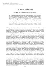
sector. On a large scale, such a swap can thus provide an “insurance” against adverse shift of market expectations across equilibria. Here is a quote from the 2013 Per Jacobsson lecture by the former ECB president, Jean-‐Claude Trichet: “I think we have to reflect more on the reason why the purchases of Treasuries appeared appropriate in the aftermath of the crisis despite the paradox that they seem to have a modest effect on the economy as a whole […]. Such purchases might have played the role of an insurance policy against any start of materialization of the ultimate tail risk: the challenge to sovereign signatures (not only the weakest European ones) […]. The counterfactual is naturally impossible to figure out. But it is illegitimate to wonder what could have happened, in the past three years, if a number of central banks had not purchased any Treasuries, at a moment when investors and savers, losing confidence, were starting to put into question all signatures, including the traditionally unchallengeable risk-‐free?” Jean-‐Claude Trichet, 2013, p. Obviously, Trichet had in mind pictures like Figure 6, showing the holdings of gilts by the Bank of England going up to almost ¼ of the outstanding stock. Trichet’s argument takes for granted that markets do not see fiat money as defaultable. We have long understood that imperfect substitutability between monetary liabilities and other assets provides the foundations of open market operations and the effectiveness of monetary policy. The same property lies at the heart of a theory of monetary backstop. Central bank liabilities do differ from the government’s in that the former, cash and bank reserves, are a claim to cash-‐-‐-‐by its nature, fiat money is a claim on itself-‐-‐-‐and central banks can always make good on their debt by running the printing press. If you live in England, you are constantly reminded of the meaning of fiat money. Any time you use, say, a 10 pound banknote, you can read on it: the bearer of the present has the right to be paid, well, 10 pounds. The Bank of England’s website is actually quite explicit: “What is the Bank’s “Promise to Pay”? The words “I promise to pay the bearer on demand the sum of five [ten/twenty/fifty] pounds” date from long ago [...] But the value of the pound has not been linked to gold for many years, so the meaning of the promise to pay has changed. Exchange into gold is no longer possible and Bank of England notes can only be exchanged for other Bank
13
of England notes of the same face value. Public trust in the pound is now maintained by the operation of monetary policy, the objective of which is price stability.” Marco Bassetto noted that the translation into American English of the same point is much more direct and synthetic: “In God we trust”. When writing monetary models, we economists take for granted that central banks will make no discretionary attempt to tamper with the face value of monetary base. So do market participants when they form their portfolios, write contracts and trade assets. As I already mentioned, the key implication is that core central bank liabilities are exposed to inflation risk, but not to default risk-‐-‐-‐in sharp contrast with government debt, which is exposed to both inflation and default risk. But if the logic of a monetary backstop via non-‐inflationary debt purchases is particularly clear when rates are at the zero lower bound, this does not necessarily mean that such a logic needs to apply only in a liquidity trap. After all, we are facing the rise of the “new style central banking”, an era of large balance sheet, unconventional instruments, and a redefinition of the boundaries of monetary policy-‐-‐-‐see Bassetto and Messer (2013), Del Negro and Sims (2014) and Hall and Reis (2015) among many others. A relevant institutional development in the new style central banking is that monetary policymakers entertain the option to pay interest rates on reserves. Because of this option, it is not hard to envision non-‐inflationary debt purchases also under normal circumstances, when the economy is not in a liquidity trap. Namely, the central bank buys debt and issue reserves at the equilibrium interest rate, consistent with expectations of future inflation. As long as it is understood that these liabilities will always be convertible into cash/fiat money at face value, they will earn a lower interest than debt. Of course, any increase in the size of a central bank balance sheet today may create inflation risk tomorrow. To avoid this risk, enough fiscal and monetary adjustment is required to accompany the process of balance sheet reduction over time. But this is true also if the economy is initially in a liquidity trap. Under the conditions just laid out, the issuance of interest bearing reserves today will not saturate the money market, nor will affect current prices. The same strategy that we accept to work in a liquidity trap works also when the economy is not in a liquidity trap.
14
This argument, you may note, begs the question of why central banks do not issue all debt all the time. There are lots of interesting dimensions to this question, covering theory, history and the institutional design of central banking. One possible answer (by no means the only answer) is that outright default in some states of the world may be efficient, and it is advisable to keep the option open (Adams and Grill 2012). To put it in another way, if the central bank bought the whole stock of public debt, issuing its own liabilities, there could be circumstances and contingencies in which its willingness to make good on them and printing money would not be credible. But there would be circumstances and contingencies in which the central bank liabilities remain, most credibly, default-‐risk free. In this lecture, I argue that one such circumstance is defined by the vulnerability of an economy to disruptive, non-‐fundamental sovereign crises, which the central bank can avoid by an off-‐ equilibrium threat to purchase debt in sufficient quantities. In this respect, I should stress a key difference with Fiscal Theory of the Price Level. The FTPL posits that the government and the central bank are committed to ensure that all public liabilities, fiscal and monetary, are always honored at face value. Here, the argument draws a key distinction between the liabilities of the central bank and those of the government: only the former are always honored at face value. I am sure you would like to see more, from theory, history and institutional design, on the foundations of this particular property of central bank’ paper. So do I. And it is exactly for this reason that, like Paul Krugman, I still refer to it as a “mystery.” But for the purpose of our inquiry, we do have an answer to our first question in the list. A key pre-‐condition for central bank interventions in the debt market to be effective in lowering the cost of debt is: by people believing in the “mystery of the printing press”, monetary authorities can credibly issue liabilities which are default-‐risk free. If this condition fails, there is no scope for monetary backstops. We are now ready to proceed and address the other questions. Part IV How do monetary backstops work: insight from a stylized model To discuss the other questions, I will embed the “mystery of the printing press” just described in a stylized model of sovereign default and monetary backstop of government debt, and rely on some analytical and numerical results from the model. A full explanation of the model and derivation of results are in the joint paper with Luca Dedola (Corsetti and Dedola 2015).
15
The graphs I showed you before still provide useful intuition. The underlying analysis is now richer: • Default is an endogenous decision by a discretionary, benevolent fiscal authority. • Central bank debt purchases, on the one hand, and inflation, taxation and default on the other, will all be endogenously determined in equilibrium. I will keep focusing on a two period setting-‐-‐-‐intertemporal generalizations are possible but for the purpose of this lecture it is better to keep analytics at a minimum. If you want, you may think of the second period as the long run, and of variables such as the primary surplus in terms of their present discounted value. The model setup I need to tell you a bit about the model. Here is a verbal synthesis of its key features. In the economy, there are risk neutral investors, a government, and a central bank. Timeline In the first period, the asset market opens. The government supplies B bonds. The central bank may decide to intervene in the debt market and purchase a share ω of B at some intervention rate, issuing interest-‐ bearing reserves. Agents can invest in three assets. • A safe real asset in infinite supply, which yields a constant return in real terms. R denotes the corresponding nominal rate, compensating for expected inflation. • Government debt in fixed supply B: the required interest rate for investors to buy debt, RB, must compensate for both anticipated inflation and anticipated default. • Central bank reserves, if any is supplied. These are default-‐free, hence yield the safe nominal return R. In the second period, uncertainty about the state of the economy is realized. Acting independently under discretion (i.e. taking each others instruments as well as market rates as given), policymakers implement their policies: • The fiscal authority optimally sets taxes T and chooses whether or not to default at an optimal rate θ between 0 [no default] and 1 [full default]. • The central bank optimally sets inflation and, in case it had purchased debt in period 1, runs down its balance sheet by paying out interest rates on reserves in cash.
16
Agents consume net output, net of the distortionary effects of policies chosen by the policymakers.
Policy instruments and distortions All policy instruments are distortionary, and have costs in terms of output or the budget. Fiscal instruments are taxes and default. • Raising tax revenue T is distortionary: it produces a fall in output Z(T,Y) that is convex in tax revenue. Z(T,Y) is larger, and increases faster, the worse the state of the world. • Defaulting on debt at the rate θ (comprised between 0 and 1) reduces output by an exogenous amount Φ, and worsens the budget by a variable cost increasing in the size of total default ΘBRB on private investors at the rate α. Without loss of generality, the variable cost falls on the budget rather than on output (as in Calvo). The instruments of monetary policy are public debt purchases in the first period, and inflation in the second period. • Inflation produces convex costs in output C(π) (as in recent monetary economics) which are not bounded. • Debt purchases are not distortionary directly, but may foreshadow future inflation if contingent losses exceed the ability of the central bank to make good on its liabilities at the desired rate of inflation. Strategic interactions: policymakers’ preferences and fiscal backing As you may expect, the extent to which monetary backstops are credible, hence effective, depends on the interactions between fiscal and monetary authorities. The key maintained assumption in the model is that fiscal and monetary authorities operate under discretion and act independently. But having said so, the two authorities may still differ in their preferences, and may be subject to rules that favor or prevent fiscal support of the central bank in case of losses-‐-‐-‐del Negro and Sims (2014) refers to this as ‘fiscal backing’. In principle one may have many possible cases, more or less realistic in light of the institutional and historical evidence. In what follows, I will concentrate most of the analysis on the implications of fiscal backing (or lack thereof), rather than differences in preferences. Both dimensions are of course important, but by focusing on the former we get “more bang for buck.” Stochastic structure and equilibrium restrictions
17
The model assumes the simplest stochastic structure that, under mild, reasonable restrictions on probabilities and primary surpluses across states of nature, ensures the existence of well-‐behaved multiple equilibria. These are the key assumptions: • In the second period, there are three states of nature. Output can be High, Average, Low H,A,L with probability 1-‐γ, γμ, and γ(1-‐μ). • The probability of the high state is large enough (1-‐γ> α) and the primary surpluses are increasing enough across states of nature L, A and H . Having sketched the model, we are ready to roll. IV.1 “Calvo redux” I begin by showing you the economic environment against which I will assess the effectiveness of a backstop. To start with, I will shut down monetary policy altogether: I set inflation rates to zero and assume that central bank purchases no sovereign debt. Effectively, this is tantamount to engage in what we could label “Calvo redux”, that is, a modern reconsideration of Calvo 1988, redone in light of the key lessons from recent literature. The results from the exercise (similar to e.g. Lorenzoni and Werning 2014, or Nicolini et al. 2015) are shown in Figure 7. The figure plots the equilibrium interest bill of the government BRB against the initial stock of debt in the market. The lines in the plot overlap over two intervals of B, marked by a shaded area. For B comprised in these intervals, the equilibrium is not unique: under rational expectations there are two market rates that satisfy the equilibrium conditions. Start with values of B to the left of the first shaded area, where the government financing needs are low, and the equilibrium is unique. In this region, the primary surplus required to servicing public debt in full is small, and so are tax distortions relative to the fixed costs the government would incur by defaulting. The government will never find it optimal to impose haircuts on bond holders. Consistently, investors will charge the risk free rate R. For larger values of B, if the government wants to make good on its promises, higher debt costs implies higher level of distortionary taxation, hence progressively higher output losses. For an interest bill large enough, in some states of the world the welfare gains from defaulting and slashing taxes over the alternative of servicing the debt in full may overcome the fixed and variable costs of default. At that point, default becomes the optimal course of action. When B falls in the first shaded area to the left, there is an equilibrium in which default occurs only under weak fundamentals, that is, under conditions of fiscal 18
stress.5 Yet, depending on agents’ expectations, an equilibrium with no default in any state of the world is still possible. The no default equilibrium disappears for levels of B to the right of the shaded area. In this region, the cost of debt would be large enough for the government to impose a haircut in L, even if (violating rational expectations) investors charged the risk free rate. The equilibrium is unique, with default in state L only. The haircut rate quickly gets to its maximum, 100 percent. Further to the right, we have multiplicity again (the second shaded area): in one equilibrium there is fundamental default in state L only; in the other equilibrium, default occurs in both states L and A.6 Multiplicity is bad for welfare. The equilibrium with more default in more states of the world is inefficient for two reasons. First, in any state of the world in which the government repudiates its liabilities, the economy suffers default-‐related output losses and budget costs. Second, in the other states of the world, where default does not occur, higher debt costs lead to higher tax distortions. IV.2 Conventional inflation policy Would inflation be the right instrument to eliminate multiplicity? We already know the answer, but it is instructive to let the model deliver it again. In the model, I now switch on the conventional inflation policy.7 The figure 8 reproduces the economy with positive, optimally chosen, state-‐ contingent inflation. At the margin, monetary policy does make some difference-‐-‐ -‐the economy is working with an additional policy instrument in place, affecting the ranges of B at which multiplicity occurs. This difference crucially depends on the costs of inflation. The higher these costs, the closer the two graphs, with and without monetary policy, to each other. But, clearly, inflation does nothing to eliminate multiplicity. We have already discussed the reason. A bout of inflation large enough to debase debt is simply not credible. Essentially, the costs of inflation quickly reduce the welfare advantage of stealth monetary default over outright fiscal default. 5 In this equilibrium, market participants coordinate their expectations on default in the state L. The cost of debt rises, but only in this state the higher interest bill push the government across the red line, and the economy incurs the costs of default. In the other states of the world, A and H, the government will service its debt in full. Here, the high debt costs translate into more tax distortions. 6 In the figure, the position of these lines and the size of the jumps across them depend on policy distortions. If distortions grow slowly with taxation (a flat Z function), the government will tend to default for higher level of B. Yet, when default eventually becomes optimal, the haircut imposed on bond holders will tend to be larger. 7 Incidentally, in this subsection fiscal backing is not an issue, as there is no risk of balance sheet losses without central bank interventions.
19
Here, however, inflation is not ‘part of the problem’, as in Calvo 88. By our assumptions about inflation costs, there is no multiplicity in inflation rates. In the shaded areas, there are two different equilibrium haircut rates. However, once an equilibrium is selected, inflation is uniquely determined. There is only one inflation rate corresponding to a given haircut rate. The debt costs cannot rise driven by self-‐fulfilling expectations of higher inflation (for given haircut rates). Since we model a discretionary central bank, inflation will tend to be positive in equilibrium. By the first order conditions of the policy problem, inflation will tend to move together with taxation. Intuitively, the optimal plan will tend to smooth policy distortions across instruments: everything else equal, in states of nature in which taxes are relatively high, also inflation will tend to be relatively high, producing a bit more seigniorage and giving in slightly to the temptation to trim the real value of public liabilities. Depending on the cost of inflation, however, the equilibrium rates are quite small. IV.3 Unconventional balance sheet policy We finally come to our main task: assessing the role and properties of unconventional balance sheet policy. As I mentioned already, I will organize my discussion around two cases, depending on whether the treasury provides, or fails to provide, ‘fiscal backing’ to the central bank. What’s at stake with fiscal backing is apparent. When the central bank intervenes in the sovereign debt market, it exposes its balance sheet to large losses from government default risk. This is a potential problem if the treasury provides no fiscal backing under any circumstances. To be clear: central banks do not go bankrupt. They can always print the fiat money they have promised. The problem is: facing large losses, the use of the printing press to make good on its own nominal liabilities may become inconsistent with the central bank’s desired inflation goals. If inflation must adjust residually to make up for balance sheet losses, it cannot at the same time be set efficiently. This will indeed be the case when balance sheet losses are large relative to the central bank’s assets and the present discounted value of its income flows-‐-‐-‐this is, basically, seigniorage not committed to the treasury. You may observe that, at least among advanced countries, not only are central banks held responsible for backing their own liabilities. Also, there are rules restricting the modalities and size of fiscal transfers from and to the central bank. In principle, all this is against fiscal backing. However, rules can be and frequently are modified ex post, especially in a crisis situation. At a minimum, during crisis fiscal authorities typically forgo
20
seigniorage revenue, suspending the central bank’s obligation to pay it to the treasury. If push comes to shove, most central banks know that they may count on some, direct or indirect, fiscal support. For instance, they may be granted formal or informal seniority status on their holding of debt. And (why not?) they may be recapitalized. In short, fiscal backing may not be as unrealistic as suggested by norms and regulations in place during non-‐crisis times. I will start with it as my benchmark case. IV.3.a Monetary backstop under fiscal backing With fiscal backing eliminating immediate balance sheet considerations from the policy equations, the monetary authorities can always pursue their preferred efficient inflation policy (n the model, according to the first order conditions of the policy plan).8 Concretely, fiscal backing means that possible balance sheet losses constrain neither • the central bank’s willingness to intervene ex ante, nor • its ability to pursue its desired inflation objectives over time. Figure 9 represents the equilibrium effects of central bank debt purchases. On the y-‐axis is the initial financing need of the government B, on the ex-‐axis the share of it bought by the central bank, ω in period 1. In the figure, different colors identify combinations of B’s and ω’s that lead to different equilibria. In the white region, there is a unique equilibrium with no default. Turquoise marks multiplicity, with either no default or default in L only. Light blue corresponds to a unique equilibrium with default in L only. Red to multiple equilibria with default either in L or in L and A. Finally, dark blue on the north-‐west marks a dreadful unique equilibrium with default in L and A. The different equilibria shown in the previous figure can be seen along the y-‐ axis. Stating from B=0 and moving upwards: a unique equilibrium with no default is followed by multiple equilibria with either no default or default in L. Then there is again a unique equilibrium with default in L only, followed by multiple equilibria with default either in L or both in L and in A. Conversely, for each level of initial debt on the Y-‐axis, one can read the effect of central bank interventions of increasing size by moving rightwards, horizontally, across the graph. 8 On analytical grounds, under fiscal backing, the two authorities basically end up consolidating their budget constraint. Since in the model they also share the same objective function, even if they act independently, the optimal discretionary policy plan will overlap with the case of cooperative policymaking.
21
For an initial debt in the turquoise area, it takes interventions above 50 percent of the financing needs of the government to rule out multiplicity and guarantee a unique equilibrium with no default. For an initial debt in the red area, again, interventions with ω above 50 percent can enforce a unique equilibrium in which default occurs only under fundamental stress. By the logic of the backstop, if a central bank stands ready to purchase debt on a sufficient scale in period 1, this is enough to coordinate investors’ expectations away from the bad equilibrium, in which a high interest rate causes socially inefficient default. Here is a key insight from the model. Monetary backstops rule out multiplicity of equilibria, without necessarily ruling out default under fundamental fiscal stress. If cumulative debt is high enough and the economy turns out to perform poorly, default can still happen under a central-‐bank backstop. Debt restructuring per se is no “proof that the backstop does not work”, nor necessarily undermines its credibility.9 Most crucially, a central bank backstop cannot be mistaken for the solution to a country’s fiscal problems. To the extent that the purchase of debt is an off-‐equilibrium threat, fundamental default is immaterial, ex post, for the balance sheet of the central bank and the implicit commitment by the fiscal authority to provide backing. It is not immaterial ex ante, since the way losses are dealt with off-‐equilibrium determines the credibility of the central bank policy. Now, you may note from the graph that very large interventions, large enough to bypass the turquoise area to the right, can enforce a unique equilibrium with no default at all, even at a high initial level of B. For this to be possible, however, the backstop requires different modalities of implementation. An off-‐equilibrium threat to buy debt would not work: we know that, with B high enough, weak fundamentals can make the interest bill unsustainable even if investors charged the risk free rate. To enforce an equilibrium with no default, the central bank must intervene and actually purchase the debt in the first period. No surprise here. This limit result is rooted in the logic of interventions as a swap in liabilities, by which the central bank injects policy commitment to repay debt. 9 On default on domestic sovereign debt, see e.g. Reinhardt and Rogoff (2013). 22
Welfare comparisons in this limit case are nonetheless tricky. We know that default may be efficient under commitment, as explained e.g. by Adams and Grill (2012). But in our economy, default occurs under discretionary policy. Hence, on anticipation of default, expectations tend to raise the costs of debt inefficiently, creating the premise for high, welfare damaging, tax-‐ and inflation-‐related distortions.10 Are debt purchases inflationary? Recall the main implications of fiscal backing: as long as the treasury ensures fiscal backing to the central bank, a monetary backstop to government debt cannot compromise the central bank’s ability to set inflation efficiently. There is no reason to the central bank to set it not in accord to its own preferences. . Most importantly, as an off equilibrium threat, a backstop requires no purchases ex ante of debt. At ω =0, there is very little variation in inflation across the equilibria in the first and the second graph. Inflation considerations take center stage, however, when fiscal backing is not granted. IV.3.b Can a monetary backstop be credible in the absence of fiscal backing? When I first thought of backstop without fiscal backing, it came natural to me to think of prospective inflation as a potential reason for the central bank not to intervene. The argument goes like this. Debt purchases raise the risk of losses, and these losses in turn cause inefficiently large adjustment in state-‐contingent inflation. For an increasing scale of purchases, rising costs of prospective inflation may at some point reduce social welfare under a backstop below social welfare in a belief-‐driven crisis. Then, in response to a shift in coordination of market expectations across equilibria, the central bank would prefer not to engage. Large-‐scale interventions would simply be not credible. This argument is compelling because, as made clear above, monetary backstops do not necessarily eliminate fundamental default. Ruling out belief-‐driven crises does not completely eliminate the risk of balance sheet losses. Actually, one may be tempted to look for a sort of balancing act: to be credible, interventions must be large enough to eliminate self-‐fulfilling default, but not too large, as to create the need for extremely high inflation under fundamental default. Well, something is missing from the argument. The model actually turns the above conjecture on its head. 10 See the discussion by Roch and Uhligh (2012)
23
I will now present results from the model imposing that the fiscal authority credibly sticks to a strict “no-‐fiscal-‐backing rule” under any circumstances. Without loss of generality, I assume that the central bank buys government debt at the default-‐free nominal rate R, and default always happens under a pari-‐ passu rule: the same haircut rate is applied to both private investors and the central bank. In this environment, the no-‐fiscal backing constraint becomes binding even at moderate levels of central bank purchases. For the central bank, the moment it buys non-‐negligible amount of debt, it will no longer be possible to implement its efficient inflation policy: inflation will have to be adjusted residually, to make sure that the central bank liabilities are honored, if only in nominal terms. The results from the exercise are shown by Figure 11. The no-‐default equilibrium is all over the place, for most B’s and ω’s-‐-‐-‐with the notable exception of a small region in the upper left corner of the graph, where debt is quite high, and interventions quite low. The reason is straightforward. As long as the fiscal authority cares about inflation costs, the inflationary consequences of debt repudiation raise overall default-‐related costs to prohibitively high levels. In other words, because the central bank internalizes the inflationary consequences of fiscal backing, budget separation strengthens its ability to provide a monetary backstop. By igniting high prospective inflation under weak fundamentals, central bank interventions today play the role of a commitment device for the government not to default under any circumstances. They activate an automatic deterrent against default reminiscent of Stanley Kubrick’s Dr. Strangelove. I should stress a key difference between balance sheet policies under no fiscal backing and the contingent inflation plan envisioned in Part II above. Here, in reaction to an incipient debt crisis, the central bank acts immediately, and buys debt. It is via debt purchases in period 1 that the central bank locks in future inflation contingent on default, which in turn eliminates the bad equilibrium because of the high costs of inflation. For the strategy discussed in Part II to work, the central bank needs to convince investors that it will act in the future, when fiscal stress materializes, in spite of the high costs of inflation. The difference in the time of policy action and the role of inflation costs across strategies is substantial. So, our sharpest result so far: with the two authorities sharing the same social welfare function, high prospective inflation with no fiscal backing does not discourage central bank purchases at all. On the contrary, it strengthens their credibility.
24
What if the two authorities have different preferences? If the fiscal authority does not care about inflation at all, the costs of inflation no longer influence the decision to default. For the reasons explained above, the prospective loss of control over inflation contingent on a fundamental default may make the central bank reluctant to intervene-‐-‐-‐substantially narrowing the scope for backstop policies. With heterogeneity in policymakers’ preferences, thus, fiscal backing plays a much more important role, as a precondition for a successful backstops. Heterogeneity in policy preferences and restrictions on fiscal backing are obviously relevant to the analysis of the Eurozone. For the sake of argument: suppose fundamental default by a country could create large losses for the ECB that, absent fiscal backing, would produce some inflationary consequences at the EZ level. Even if this were the case, these consequences would be way too diffuse and too small to be a deterrent to debt repudiation by a national government, regardless of its attitude on inflation. As is well known, the OMTs program is only accessible conditional on the country entering a program with the European Stability Mechanism (ESM). It is tempting to interpret OMTs’ “conditionality” as a form of insurance against the consequences of no fiscal backing. Requiring a country to be in a ESM program as a precondition to benefit from the OMTs program, can be seen as a way to minimize fundamental default, once belief-‐driven crises are taken off the table. IV.5 Discussion There are a number of factors and considerations that may complicate the design of a successful backstop. These include multiplicity in inflation, non-‐market interventions by the central bank and “moral hazard.” Given the time constraint, I will only touch upon them. Multiplicity in inflation In the model above, the success of the backstop rests on uniqueness of inflation. As we learnt from Calvo 1988, this is a problem when the costs of inflation are (perceived to be) bounded.11 In this case, even if the threat of debt purchases by the central bank is successful in ruling out self-‐fulfilling outright default for relatively good fundamentals, under rational expectations there could still be more than one equilibrium inflation rate, hence more than one equilibrium nominal interest rate. Bad belief-‐ driven equilibria will be of the kind studied by Calvo, with high nominal rate, high debt costs, high inflation. A discussion of this point is quite relevant in today’s policy debate. There are a number of people who advocate central bank interventions in the debt market 11 Another source of multiplicity is the Laffer Curve.
25
on unbounded scale, essentially claiming that inflation risks should be ignored because inflation costs are overstated as in reality they are low and bounded. Whether or not one shares these beliefs, it is important to be aware of their implications. If one stresses low and bounded social costs of inflation as “the” motivation for large central bank interventions in the debt market, he/she needs to accept the lesson from Calvo 1988: belief-‐driven equilibria would be actually be much more pervasive. Low costs of inflation are no strong foundations of a backstop. Non-‐market interventions Another claim, often voiced in the debate, holds that the central bank has a number of instruments to fight destabilizing speculation, in addition to market interventions. By law or suasion-‐-‐-‐the argument goes-‐-‐-‐the central bank can always push private banks to hold sovereign debt, and/or they can force banks to hold monetary reserves indefinitely, in large amounts-‐-‐-‐no need to pay interest on reserves to compensate banks for inflation risks. The problem in this view is apparent. Markets may start to perceive the risk of stealth default on the central bank liabilities, in the form of, say, implicit changes in the terms of its financial contracts with banks. If a central bank is expected to tamper with its liabilities, in any form, markets would stop considering its liabilities as default free. The logic of self-‐fulfilling beliefs would then apply to a discretionary central bank as well as to the government. Moral Hazard The main issue here is whether and how a backstop could feed opportunistic behavior by the fiscal authority, exacerbating fiscal fragility and therefore the likelihood of (fundamental) default.12 This widely debate issue would that deserves a much deeper discussion. I just go over the basics. Conceptually, backstops are distinct from bailouts in the form of contingent transfers. There is a long-‐standing literature emphasizing that a backstop may actually strengthen the incentives for a government to do the right thing-‐-‐-‐the opposite of the “moral hazard” consequences of a bailout (see Morris and Shin 2006, Corsetti et al. 2005 and Corsetti and Dedola 2011 among others). This is because the possibility of belief-‐driven crises tends to reduce the expected future benefits from current (costly) policy initiatives. Nonetheless, a key problem is that a backstop does not necessarily eliminate fundamental default. With weak fundamentals creating fiscal stress, the central bank runs the risk of being drawn into quite a different game, a “Game of 26
Bailouts” and/or straight debt monetization a la Sargent and Wallace (1981), which may threaten its independence and ability to deliver on its objectives.13 This is why backstops do require some form of conditionality, and the clear definitions of rules of engagement and disengagement for the central bank. A “Game of Bailouts” risk, however, is hardly a sufficient reason to leave a country out in the cold of non-‐fundamental sovereign crises. Conclusions Large-‐scale monetary experiments do not happen very often, and should never go wasted in policy and academic research. Not surprisingly, because of its large financial and economic impact, the ECB’s OMTs program has prompted a number of empirical and policy-‐related studies, and raised key questions in monetary theory and the institutional design of central banks. These questions are related to but conceptually distinct from other policies also motivating a significant expansion of the balance sheet of central banks, like Quantitative Easing or Credit Policies-‐-‐-‐the so called “new style central banking” see Bassetto Messer (2013), Del Negro and Sims (2014) and Hall and Reis (2015), among others. In essence it is all about monetary policy: different instruments and strategies share a key common feature, they all rely on the imperfect substitution between central bank liabilities and government or private sector bonds. By way of example, the ability of the central bank to borrow in better terms than the private sector features prominently in recent work by Gertler and Karadi (2011). This lecture today, and the paper I wrote with Luca Dedola, are meant to contribute to bridging the gap between monetary theory and the practice of monetary policy, made apparent by the ECB initiative with the OMTs, but in retrospect also highlighted by the heavy engagement of many central banks in their own sovereign debt market. This gap is in part related to the intellectual inheritance from early work focused on contingent debt monetization as ‘the’ way to implement a monetary backstop. In a modern and complex economy, with a high degree of financial development, central banks can use more, unconventional, instruments. Some may argue that the mystery of the printing press analyzed in this lecture is only effective in a deep crisis situation with policy rates at the zero lower bound, and cannot be generalized to other circumstances. Even if this were true, understanding the mechanism would already be worth the effort. The toughest challenge is however yet to come. As advanced economies are hopefully moving out of a liquidity trap, they do so with an uncomfortably high 13 In a multi-‐country setting, the counterparty of this problem is transfers in the form of contingent bailout, because of fear of negative spillovers, see Tirole (2015).
27
stock of public (and private) liabilities. They thus remain potentially vulnerable to self-‐fulfilling debt crises. We do need to understand the conditions under which, outside a liquidity trap, central banks can still be in a position to insure countries, as President Trichet would say, “against the ultimate tail risk: the challenge to sovereign signatures.” References Adam, K. and M. Grill, (2012). "Optimal Sovereign Default," CEPR Discussion Papers 9178, C.E.P.R. Discussion Papers. Aguiar M., M. Amador, E. Farhi and G. Gopinath (2012). Crisis and Commitment: Inflation Credibility and the Vulnerability to Sovereign Debt Crises, mimeo Bacchetta P., E. Perazzi and E. Van Wincoop (2015). “Self-‐fulfilling Debt Crises: can Monetary Policy Help?” CEPR DP 10609 Bassetto M. and T. Messer (2013). “Fiscal Consequences of Paying Interest on Reserves” Federal Reserve Bank of Chicago, 2013-‐04 Calvo G. (1988). "Servicing the Public Debt: The Role of Expectations" American Economic Review 78(4): 647-‐661 Cole, H. L. and Kehoe, T. (2000). "Self-‐Fulfilling Debt Crises" Review of Economic Studies, 67: 91-‐-‐116 Cohen, D. and S. Villemot (2011). "Endogenous debt crises". CEPR Discussion Paper no. 8270. London, Centre for Economic Policy Research. Cooper R. and A. Camous (2014) Monetary Policy and Debt Fragility, NBER Working Paper 20650. Corsetti G., B. Guimaraes and N. Roubini (2006) “International Lending of Last Resort and Moral Hazard: a model of IMF’s catalytic finance”, Journal of Monetary Economics, 53: 441-‐471. Corsetti G. and L. Dedola (2011). "Fiscal Crises, Confidence and Default: A Bare-‐ bones Model with Lessons for the Euro Area". mimeo, Cambridge University. Corsetti G. and L. Dedola (2013), “The Mystery of the Printing Press: Monetary Policy and Self-‐fulfilling Debt crises” with Luca Dedola, mimeo Cruces, J. and C. Trebesch (2013). "Sovereign Defaults: The Price of Haircuts", American Economic Journal: Macroeconomics, 5(3), pp. 85–117. Del Negro, M. and C. Sims (2014). "When does a central bank balance sheet require fiscal support?", Staff Reports 701, Federal Reserve Bank of New York, forthcoming in Carnegie-‐NYU-‐Rochester Series.
28
Gertler M. and P. Karadi (2011). "A Model of Unconventional Monetary Policy", Journal of Monetary Economics 58: 17-‐34. Hall, R.E. and R. Reis (2015), “Maintaining Central-‐Bank Financial Stability under New-‐Style Central Banking”. CEPR Discussion Papers 10741, C.E.P.R. Discussion Papers. Lorenzoni, G. and I. Werning, (2014). "Slow moving debt crises." mimeo. Morris, St. and H. Shin (2006). "Catalytic finance: When does it work?" Journal of International Economics, 70(1):161-‐177. Nicolini, JP., P. Teles, J. L. Ayres, and G. Navarro (2015). "Sovereign Default: The Role of Expectations" Working Papers 723, Federal Reserve Bank of Minneapolis. Olivier J. (2012). "Fiscal Challenges to Monetary Dominance in the Euro Area: A Theoretical Perspective" mimeo. Reinhart, C. M. and Rogoff, K. S. (2011), "The Forgotten History of Domestic Debt." The Economic Journal, 121(552): 319-‐350. Roch F. and H. Uhlig (2011). "The Dynamics of Sovereign Debt Crises and Bailouts", mimeo Sargent T. and N. Wallace (1981). "Some unpleasant Monetarist Arithmetic", Quarterly Review, Federal Reserve Bank of Minneapolis, 5(3): 1-‐17. Tirole J. (2012). "Country Solidarity, Private Sector Involvement and the Contagion of Sovereign Crises," mimeo
29
0"
30 1987M1" 1987M7" 1988M1" 1988M7" 1989M1" 1989M7" 1990M1" 1990M7" 1991M1" 1991M7" 1992M1" 1992M7" 1993M1" 1993M7" 1994M1" 1994M7" 1995M1" 1995M7" 1996M1" 1996M7" 1997M1" 1997M7" 1998M1" 1998M7" 1999M1" 1999M7" 2000M1" 2000M7" 2001M1" 2001M7" 2002M1" 2002M7" 2003M1" 2003M7" 2004M1" 2004M7" 2005M1" 2005M7" 2006M1" 2006M7" 2007M1" 2007M7" 2008M1" 2008M7" 2009M1" 2009M7" 2010M1" 2010M7" 2011M1" 2011M7" 2012M1" 2012M7" 2013M1" 2013M7" 2014M1"
Percentage)
Figure 1
30"
25"
Long-Term)Government)Bond)Yields)
20" Belgium"
Ireland"
15" Greece"
Spain"
France"
10" Italy"
Germany"
5" Netherlands"
Portugal"
Finland"
Year)
Figure 2
Cost of debt
Self-fulfilling debt crisis
(B•R ) E ____B
(1+π)
Critical threshold
No default is expected Investors charge risk free rate R
Gov't financing needs
B
Figure 3 Cost of debt
Self-fulfilling debt crisis
____B) E (B•R (1+π)
Self-fulfilling expectations of default in state L Investors charge high rate RB Critical threshold
No default is expected Investors charge risk free rate R
Gov't financing needs
B
Figure 4
Contingent inflationary debasement Cost of debt (B•R ) E ____B (1+π)
Self-fulfilling expectations of default in state L Investors charge high rate RB
π Critical threshold
No default is expected Investors charge risk free rate R
B
Gov't financing needs
31
Figure 5 Cost of debt
Central Bank Interventions
(B•RB) E ____ (1+π)
Self-fulfilling expectations of default in state L Investors charge high rate RB
[(1-ω)•RB)+ω•R]•B Critical threshold
No default is expected Investors charge risk free rate R
B
Gov't financing needs
Figure 6 APF Asset Purchase Facility
BoE gilt holdings (% of UK government debt) 25 20 15 10 5 0 2009 2009 2010 2010 2011 2011 2012 2012 2013 2013 2014 2014 2015 Jan Jul Jan Jul Jan Jul Jan Jul Jan Jul Jan Jul Jan
http://www.ons.gov.uk/ons/publications/re-‐reference-‐tables.html?edition=tcm%3A77-‐380428
32
Figure 7
Figure 8
33
Figure 9
34
Figure 11