The Niceness of Unique Sink Orientations Bernd Gärtner and Antonis Thomas Department of Computer Science Institute of Theoretical Computer Science, ETH Zürich 8092 Zürich, Switzerland {gaertner, athomas}@inf.ethz.ch
Abstract Random Edge is the most natural randomized pivot rule for the simplex algorithm. Considerable progress has been made recently towards fully understanding its behavior. Back in 2001, Welzl introduced the concepts of reachmaps and niceness of Unique Sink Orientations (USO), in an effort to better understand the behavior of Random Edge. In this paper, we initiate the systematic study of these concepts. We settle the questions that were asked by Welzl about the niceness of (acyclic) USO. Niceness implies natural upper bounds for RE and we provide evidence that these are tight or almost tight in many interesting cases. Moreover, we show that RE is polynomial on n at least nΩ(2 ) many (possibly cyclic) USO. As a bonus, we describe a derandomization of RE which achieves the same asymptotic upper bounds with respect to niceness. 1998 ACM Subject Classification F.2.2 Nonnumerical Algorithms and Problems, G.2.1 Combinatorics Keywords and phrases random edge, unique sink orientation, random walk, reachmap, niceness Digital Object Identifier 10.4230/LIPIcs.xxx.yyy.p
1
Introduction
One of the most prominent open questions in the theory of optimization is whether linear programs can be solved in strongly polynomial time. In particular, it is open whether there exists a pivot rule for the simplex method whose number of steps can be bounded by a polynomial function of the number of variables and constraints. For most deterministic pivot rules discussed in the literature, exponential lower bounds are known. The first such bound was established for Dantzig’s rule by Klee and Minty in their seminal 1972 paper [20]; this triggered a number of similar results for many other rules; only in 2011, Friedmann solved a longstanding open problem by giving a superpolynomial lower bound for Zadeh’s rule [8]. On the other hand, there exists a randomized pivot rule with an expected subexponential number of steps in the worst case. This bound was found independently by Kalai [18] as well as Matoušek, Sharir and Welzl [23] in 1992. Interestingly, the proofs employ only a small number of combinatorial properties of linear programs. As a consequence, the subexponential upper bound for the Random Facet pivot rule holds in a much more general abstract setting that encompasses many other (geometric) optimization problems for which strongly polynomial algorithms are still missing [23]. This result sparked a lot of interest in abstract optimization frameworks that generalize linear programming. The most studied such framework, over the last 15 years, is that of unique sink orientations (USO). First described by Stickney and Watson already in 1978 as abstract models for P-matrix linear complementarity problems (PLCPs) [28], USO were revived by Szabó and Welzl in 2001 [29]. Subsequently, their structural and algorithmic properties were studied extensively ([26],[27],[22],[13],[7],[2],[16],[14],[19],[17]). In a nutshell, © Bernd Gärtner and Antonis Thomas; licensed under Creative Commons License CC-BY Conference title on which this volume is based on. Editors: Billy Editor and Bill Editors; pp. 1–20 Leibniz International Proceedings in Informatics Schloss Dagstuhl – Leibniz-Zentrum für Informatik, Dagstuhl Publishing, Germany
2
The Niceness of Unique Sink Orientations
a USO is an orientation of the n-dimensional hypercube graph, with the property that there is a unique sink in every subgraph induced by a nonempty face. The algorithmic problem associated to a USO is that of finding the unique global sink, in an oracle model that allows us to query any given vertex for the orientations of its incident edges. In recent years, USO have in particular been looked at in connection with another randomized pivot rule, namely Random Edge (RE for short). This is arguably the most natural randomized pivot rule for the simplex method, and it has an obvious interpretation also on USO: at every vertex pick an edge u.a.r. from the set of outgoing edges and let the other endpoint of this edge be the next vertex. The path formed constitutes a random walk. Ever since the subexponential bound for Random Facet was proved in 1992, researchers have tried to understand the performance of Random Edge. This turned out to be very difficult, though. Unlike Random Facet, the Random Edge algorithm is non-recursive, and tools for a successful analysis were simply missing. A superexponential lower bound on cyclic USO (actually, PLCPs) was shown by Morris in 2002 [25], but there was still hope that Random Edge might be much faster on acyclic USO (AUSO). Only in 2006, a subexponential lower bound for Random Edge on AUSO was found by Matoušek and Szabó [24] and, very recently, pushed further by Hansen and Zwick [17]. While these are not lower bounds for actual linear programs, the results demonstrate the usefulness of the USO framework: it is now clear that the known combinatorial properties of linear programming are not enough to show that Random Edge is fast. Note that, in 2011, Friedmann, Hansen and Zwick proved a subexponential lower bound for Random Edge on actual linear programs, “killing” yet another candidate for a polynomial-time pivot rule [9]. Still, the question remains open whether Random Edge also has a subexponential upper bound. As there already is a subexponential algorithm, a positive answer would not be an algorithmic breakthrough; however, as Random Edge is notoriously difficult to analyze, it might be a breakthrough in terms of novel techniques for analyzing this and other randomized algorithms. The currently best upper bound on AUSO is an exponential improvement over the previous (almost trivial) upper bounds, but the bound is still exponential, 1.8n [16]. In this paper, we initiate the systematic study of concepts that are tailored to Random Edge on USO (not necessarily only AUSO). These concepts — reachmaps and niceness of USO — were introduced by Welzl [30], in a 2001 workshop as an interesting research direction. At that time, Random Edge was considered hopeless, though; hence, this research direction remained unexplored and the problems posed by Welzl remained open. Now that the understanding of Random Edge on USO has advanced a lot we hope that these “old” concepts will finally prove useful, probably in connection with other techniques. The reachmap of a vertex is the set of all the coordinates it can reach with a directed path, and a USO is i-nice if for every vertex there is a directed path of length at most i to another vertex with smaller reachmap. Welzl pointed out that the concept of niceness provides a natural upper bound for the Random Edge algorithm. Furthermore, he asks the following question: “Clearly every unique sink orientation of dimension n is n-nice. Can we do better? In particular what is the general niceness of acyclic unique sink orientations?” We settle these questions, in Section 4, by proving that for AUSO (n − 2)-nice is tight, meaning that (n − 2) is an upper bound on the niceness of all AUSO and there are AUSO that are not (n − 3)-nice. For cyclic USO we argue that n-nice is tight. In Section 2, we give the relevant definitions and in Section 3 we show the upper bound of O(ni+1 ) for the number of steps RE takes on an i-nice USO. In addition, we describe a derandomization of RE which also takes at most O(ni+1 ) on an i-nice USO, thus matching the behavior of RE. Finally, we include two brief notes in Section 3. The first argues that RE needs at most
B. Gärtner and A. Thomas
3
n
quadratic steps in at least nΘ(2 ) many, possibly cyclic, USO. The second that RE can solve the AUSO instances that have been designed as lower bounds for other algorithms (e.g. Random Facet [21],[10] or Bottom Antipodal [27]) in polynomial time. All the necessary details for these two notes are provided in Appendices C and D respectively.
2
Preliminaries
We use the notation [n] = {1, . . . n}. Let Qn = 2[n] be the set of vertices of the n-dimensional hypercube. A vertex of the hypercube v ∈ Qn is denoted by the set of coordinates it contains. The symmetric difference of two vertices, denoted as v ⊕ u is the set of coordinates in which they differ. Now, let J ∈ 2[n] and v ∈ Qn . A face of the hypercube, FJ,v , is defined as the set of vertices that are reached from v over the coordinates defined by any subset of J, i.e. FJ,v = {u ∈ Qn |v ⊕ u ⊆ J}. The dimension of the face is |J|. We call edges the faces of dimension 1, e.g. F{j},v , and vertices the faces of dimension 0. The faces of dimension n − 1 are called facets. For k ≤ n we call a face of dimension k a k-face. Let v, u ∈ Qn . By |v⊕u| we denote the Hamming distance (size of the symmetric difference) of v and u. Given v ∈ Qn , we define the neighborhood of v as N (v) = {u ∈ Qn | |v ⊕ u| = 1}. Now, let ψ denote an orientation of the edges of the n-dimensional hypercube. Let v, u ∈ Qn . j The notation v − → u (w.r.t ψ) means that F{j},v = {v, u} and that the corresponding edge is oriented from v to u in ψ. Sometimes we write v → u, when we do not care on which j coordinate is the edge directed from v to u. An edge v − → u is forward if j ∈ u and otherwise we say it is backward. We say that ψ is a Unique Sink Orientation (USO) if every non-empty face has a unique sink. In the rest we write n-USO to mean a USO over Qn . Here n is always used to mean the dimension of the corresponding USO. Consider a USO ψ; we define its outmap sψ , in the spirit of Szabó and Welzl [29]. The outmap is a function sψ : Qn → 2[n] , defined by j
sψ (v) = {j ∈ [n]|v − → v ⊕ {j}} for every v ∈ Qn . A sink of a face FJ,v is a vertex u ∈ FJ,v , such that sψ (u) ∩ J = ∅. We mention the following lemma w.r.t. the outmap function. I Lemma 1 ([29]). For every USO ψ, sψ is a bijection. The algorithmic problem for a USO ψ is to find the global sink, i.e. find t ∈ Qn such that sψ (t) = ∅. The computations take place in the vertex oracle model: We have an oracle that given a vertex v ∈ Qn , returns sψ (v) (vertex evaluation). This is the standard computational model in the USO literature and all the upper and lower bounds refer to it. Reachmap and niceness. We are now ready to define the central concepts of this paper. Given vertices v, u ∈ Qn we write v u if there exists a directed path from v to u (in ψ). We use d(v, u) to denote the length of the shortest directed path from v to u; if there is no such path then we have d(v, u) = ∞ and otherwise we have d(v, u) ≥ |v ⊕ u|. The following lemma is well-known and easy to prove by induction on |v ⊕ u|. I Lemma 2. For every USO ψ, let F ⊆ Qn be a face and u the sink of this face. Then, for every vertex v ∈ F we have d(v, u) = |v ⊕ u|. Subsequently, we define the reachmap rψ : Qn → 2[n] , for every v ∈ Qn , as: [ rψ (v) = sψ (v) {j ∈ [n]|∃u ∈ Qn s.t. v u and j ∈ sψ (u)}. Intuitively, the reachmap of a vertex contains all the coordinates that the vertex can reach with a directed path. We say that vertex v ∈ Qn is i-covered by vertex u ∈ Qn , if d(v, u) ≤ i
4
The Niceness of Unique Sink Orientations
and rψ (u) ⊂ rψ (v) (proper inclusion). Then, we say that a USO ψ is i-nice if every vertex v ∈ Qn (except the global sink) is i-covered by some vertex u ∈ Qn . Of course, every n-USO ψ is n-nice since every vertex v is n-covered by the sink t. Moreover, rψ (v) ⊇ v ⊕ t, for every vertex v ∈ Qn . It is not difficult to observe that every USO at 1 or 2 dimensions is 1-nice, but the situation changes at 3 dimensions. Consider the illustration at the figure below. 2 3 1 (a)
(b)
(c)
Figure 1 Examples of 3-dimensional USO: (a) Klee-Minty, which is 1-nice. (b) The only 2-nice 3-dimensional AUSO which is not 1-nice. (c) The only cyclic USO in 3 dimensions, which is 3-nice.
Let us note that the AUSO in Figure 1(b) is the largest AUSO which is not (n − 2)-nice. As we prove in Theorem 8, every n-AUSO with n ≥ 4 is (n − 2)-nice. Algorithmic properties of the reachmap. Our focus lies mostly on the concept of niceness. Nevertheless, we briefly discuss some of the algorithmic properties of the reachmap here. It was proved by the authors, in [14], that when given an AUSO ψ described succinctly by a Boolean circuit, and two vertices s and t, deciding if s t is P SP ACE-complete. More recently, Fearnley and Savani [6] proved that deciding whether the Bottom Antipodal algorithm (this is the algorithm that from a vertex v jumps to vertex v ⊕ sψ (v)), started at vertex v will ever encounter a vertex v 0 such that j ∈ sψ (v 0 ), for a given coordinate j, is P SP ACE-complete. This line of work was initiated in [1] and further developed in [4] and [5] and aims at understanding the computational power of pivot algorithms [6]. Below, we provide a related theorem: it is P SP ACE-complete to decide if a coordinate is in the reachmap of a given vertex in an AUSO. It is, thus, computationally hard to discover the reachmap of a vertex. I Theorem 3. Let ψ be an n-AUSO (described succinctly by a Boolean circuit), v ∈ Qn and j ∈ [n]. It is P SP ACE-complete to decide whether j ∈ rψ (v). The theorem follows from the results of [14] that we mention above. A proof is included in Appendix B. Finally, we want to note that it is natural to upper bound algorithms on AUSO by the reachmap of the starting vertex. Any reasonable path-following algorithm that solves an AUSO ψ in cn steps, for some constant c, can be bounded by c|rψ (s)| where s is the starting vertex. The reason is that the algorithm will be contained in the cube Frψ (s),s of dimension |rψ (s)|. Moreover, we claim that this is also possible for algorithms that are not path-following. As an example we give in Appendix E a variant of the Fibonacci Seesaw algorithm of [29] that runs in time c|rψ (s)| for some c < φ (the golden ratio).
3
Random Edge on i-nice USO
In this section we describe how RE behaves on i-nice USO. We give a natural upper bound and argue that it is tight or almost tight in many situations. In addition, we give a simple derandomization of RE, which asymptotically achieves the same upper bound. Firstly, we consider the following natural upper bound.
B. Gärtner and A. Thomas
5
I Theorem 4. Started at any vertex of an i-nice USO, Random Edge will perform an expected number of at most O(ni+1 ) steps. Proof. For every vertex v, there is a directed path of length at most i to a target t(v), some fixed vertex of smaller reachmap. At every step, we either reduce the distance to the current target (if we happen to choose the right edge), or we start over with a new vertex and a new target. The expected time it takes to reach some target vertex can be bounded by the expected time to reach state 0 in the following Markov chain with states 0, 1, . . . , i (representing distance to the current target): at state k > 0, advance to state k − 1 with probability 1/n, and fall back to state i with probability (n − 1)/n. A simple inductive proof Pi shows that state 0 is reached after an expected number of k=1 nk = O(ni ) steps. Hence, after this expected number of steps, we reduce the reachmap size, and as we have to do this at most n times, the bound follows. J Already, we can give some first evidence on the usefulness of niceness for analyzing RE: Decomposable orientations have been studied extensively in literature. The fact that RE terminates in O(n2 ) steps on them has been known at least since the work of WilliamsonHoke [31]. Let a coordinate be combed if all edges on this coordinate are directed the same way. Then, a cube orientation is decomposable if in every face of the cube there is a combed coordinate. The class of decomposable orientations, known to be AUSO, contains the Klee-Minty cube [20] (defined combinatorially in [27]). It is straightforward to argue that such orientations are 1-nice and, thus, our upper bound from Theorem 4 is also quadratic. Moreover, quadratic lower bounds have been proved for the behavior of RE on Klee-Minty cubes [3]. We conclude that, for 1-nice USO, the upper bound in Theorem 4 is optimal. Counting 1-nice. We have mentioned that the class of decomposable USO are 1-nice. This class is the previously known largest class of USO, where Random Edge is polynomial. The n number of decomposable USO is 2Θ(2 ) . We can now argue that the class of 1-nice USO is much larger than the class of decomposable ones, and also contains cyclic USO. n
I Theorem 5. The number of 1-nice n-dimensional USO is nΘ(2 ) . The proof of the theorem above and a counting argument for decomposable USO can be found in Appendix C. The niceness of known lower bound constructions. As further motivation for the study of niceness of USO, we want to mention that RE can solve the AUSO instances that were designed as lower bounds for other algorithms in polynomial time. This is because of provable upper bounds on the niceness of those constructions. With similar arguments, upper bounds on the niceness of the AUSO that serve as subexponential lower bounds for RE can be shown; thus, RE has upper bounds on these constructions that are almost matching to the lower bounds. The upper bound for RE on the cyclic USO of Morris [25] is asymptotically matching the lower bound. We summarize the relevant information in the following table and describe the details on how to obtain it in Appendix D. Algorithm Random Facet Bottom Antipodal RE acyclic RE acyclic RE cyclic
Reference [21],[10] [27] [24] [17] [25]
Lower bound √ 2Θ( n) √ n Ω( 2 ) 2Ω(n √ 2Ω(
1/3
)
n log n) n−1 ! 2
Niceness 1 2 n1/3 √ n n
RE Upper bound O(n2 ) O(n3 ) 2O(n 2
1/3
log n)
√ O( n log n)
nO(n)
6
The Niceness of Unique Sink Orientations
3.1
A derandomization of Random Edge
Consider the join operation. Given two vertices u, v, join(u, v) is a vertex w such that u w and v w. We can compute join(u, v) as follows: by Lemma 1, there must be a coordinate, say j, such that j ∈ s(u) ⊕ s(v). Assume, w.l.o.g., that j ∈ s(u). Consider the neighbor j
u0 of u such that u − → u0 . Recursively compute join(u0 , v). It can be seen by induction on |u ⊕ v| that the join operation takes O(n) time. Similarly, we talk about the join of a set S of vertices. The join(S) is a vertex w such that ever vertex in S has a path to it. We can compute join(S) by iteratively joining every pair in S. Furthermore, let N + (v) = {u ∈ N (v)|v → u} denote the set of out-neighbors of a vertex v. In the subsequent lemma, we argue that the vertices in N + (v) can be joined with linearly many vertex evaluations. I Lemma 6. Let ψ be an n-USO and v ∈ Qn a vertex. There is an algorithm that joins the vertices in N + (v) with |sψ (v)| many vertex evaluations. Proof. First, we evaluate all the vertices in N + (v). We maintain a set of active vertices AV and a set of active coordinates AC. Initialize AV = N + (v) and AC = sψ (v). The algorithm keeps the following invariants: every vertex that gets removed from AV has a path to some l vertex in AV ; also for every vertex u s.t. v → − u, u ∈ AV if and only if l ∈ AC. Then, for each u ∈ AV : for each l ∈ AC: if l ∈ / sψ (u) and {l} = 6 (u ⊕ v) then we update AC ← AC \ {l} and AV ← AV \ (v ⊕ {l}). See Figure 2. l
u j v
w
Figure 2 We have u, w ∈ AV , l ∈ AC, l ∈ / sψ (u) and {l} 6= (v ⊕ u). Thus, the edge Fj,w has to be outgoing for w. Hence, w u and the algorithm removes w from AV and l from AC.
If in the above loop the vertex u is the sink of the face FAC,u then terminate and return v 0 = u. Of course, in this case every vertex in AV has a path to u. Otherwise the loop will terminate when there is no coordinate in AC that satisfies the conditions above. In this case we have that ∀u ∈ AV , u is the source of the face FAC\(u⊕v),u . That is, it is the source of the face spanned by the vertex and all the active coordinates AC except the one that connects it to v. In this case, we return the vertex v 0 = (v ⊕ AC). We have that every vertex in AV has a path to v 0 : this is because in any USO the source has a path to every vertex (this can be proved similarly to Lemma 2). J Using Lemma 6, we can now argue that there exists a derandomization of Random Edge that asymptotically matches the upper bound of Theorem 4. I Theorem 7. There is a deterministic algorithm that finds the sink of an i-nice n-USO ψ with O(ni+1 ) vertex evaluations. Proof. Let v be the current vertex. Consider the set Ri ⊆ 2[n] of vertices that are reachable along directed paths of length at most i from v. Since ψ is i-nice, we know that at least one of them has strictly smaller reachmap. In particular, any vertex reachable from all the vertices in Ri has a smaller reachmap. Thus, we compute the join of all the vertices in R . Pi−1 � Pi−1 i Consider the set Ri−1 . The size of Ri−1 is bounded by |Ri−1 | ≤ k=0 nk ≤ k=0 nk and, thus, |Ri−1 | = O(ni−1 ). Every vertex in Ri can be reached in one step from some vertex
B. Gärtner and A. Thomas
in Ri−1 . Assume that none of the vertices in Ri−1 is the sink; otherwise, the algorithm is finished. Then, for every vertex v ∈ Ri−1 we join N + (v) with the algorithm from Lemma 6, with O(n) vertex evaluations. Therefore, with O(ni ) vertex evaluations we have a set S of O(ni−1 ) many vertices and each v 0 ∈ S is the join of N + (v) for some vertex v ∈ Ri−1 . The next step is to join all the vertices in set S, using the algorithm at the beginning of the current section, which takes O(n) for each pair of vertices. Hence, the whole procedure will take an additional O(ni ) vertex evaluations. The result is a vertex u that joins all the vertices in Ri and thus i-covers v. Because the size of the reachmap decreases by at least one in each round, we conclude that this algorithm will take at most O(ni+1 ) steps. Finally, note that to achieve this upper bound we do not need to know that the input USO is i-nice. Instead, we can iterate through the different values of i = 1, 2, . . . without changing the asymptotic behavior of the algorithm. J
4
Bounds on niceness
In this section we answer the questions originally posed in [30] by providing matching upper and lower bounds on the niceness of USO and AUSO. For cyclic USO, the cubes designed by Morris as a lower bound for the behavior of RE [25] are n-nice and, hence, match the trivial upper bound. For the sake of conserving space, we only sketch the proof here and give explicitly an n-nice cyclic USO construction in Appendix A. The idea for such a construction is quite simple, intuitively. Let ψ be a cyclic n-USO over Qn that contains a directed cycle such that the edges that participate span all the coordinates. Then, every vertex v on the cycle has rψ (v) = [n]. Now consider the sink t and assume the n vertices in N (t) participate in the cycle. By Lemma 2, every vertex has a path to t. This path has to go through one of the vertices in N (t). It follows that every v ∈ Qn \ {t} has rψ (v) = [n]. Therefore, the vertex antipodal from t is only n-covered (by t). The Morris cyclic USO satisfies the properties described above and, thus, is n-nice. An example in 3 dimensions appears in Figure 1; this USO satisfies the properties we explain above. For the rest of this section, we will turn our attention to AUSO.
4.1
An upper bound for AUSO
We prove an upper bound on the niceness of AUSO which, as we will see in the next section, is tight. We utilize the concept of Completely Unimodal Numberings (CUN), which was studied by Williamson-Hoke [31] and Hammer et al. [15]. To the best of our knowledge, this is the first time CUN is used to prove structural results for AUSO. A CUN on the hypercube Qn means that there is an injective function φ : Qn → {0, . . . , 2n − 1} such that in every face F there is exactly one vertex v such that φ(v) < φ(u), for every u ∈ N (v) ∩ F . It is known, e.g. from [31], that for every AUSO there is a corresponding CUN, which can be constructed by topologically sorting the AUSO. In the proof of the theorem below we will use the following notation: wk is the vertex that has φ(wk ) = k, w.r.t. some fixed CUN φ. An easy, but crucial observation concerns the three lowest-numbered vertices w0 , w1 , w2 . Of course, w1 → w0 (where w0 is the global sink); otherwise, w1 would have been a second global minimum. Moreover, w2 → wj for exactly one j ∈ {0, 1}. It follows, that both w1 and w2 are facet sinks. We are ready to state and prove the following theorem. I Theorem 8. Any n-AUSO, with n ≥ 4, is (n − 2)-nice.
7
8
The Niceness of Unique Sink Orientations
Consider the vertices w0 and w1 and let e be the edge that connects them. Let w ∈ e be the unique out-neighbor of w2 and w0 the other vertex in e. W.l.o.g. assume w = ∅, w0 = {1} and w2 = {2}. The situation can be depicted as: w=∅ w0 = {1}
w2 = {2}
These three vertices have no outgoing edges to other vertices. Their outmaps and reachmaps are summarized in the table below. vertex w=∅ w0 = {1} w2 = {2}
outmap ⊆ {1} ⊆ {1} = {2}
reachmap ⊆ {1} ⊆ {1} ⊆ {1, 2}
is sink of the facet F[n]\{1},w F[n]\{1},w0 F[n]\{2},w2
More precisely, the reachmap of w2 is {2} if w = w0 , and it is {1, 2} if w = w1 . I Lemma 9. With w, w0 as above, let v ∈ Qn \ {w0 , [n]}. Then v is (n − 2)-covered by some vertex in {w, w0 , w2 }. Proof. Vertex w1 is covered by w0 and w2 by w0 or w1 , so assume that v is some other vertex. If v neither contains 1 nor 2, then v is in the facet F[n]\{1},w . Hence, d(v, w) = |v ⊕ w| ≤ n − 2. This is because F[n]\{1},w is (n − 1)-dimensional and 2 ∈ / v. Any coordinate that is part of the corresponding path is in the reachmap of v but not of w (whose reachmap is a subset of {1}). Hence, v is (n − 2)-covered by w. If v contains 1, then v is in the facet F[n]\{1},w0 , and |v ⊕ w0 | ≤ n − 2 since v 6= [n]. As before, this implies that v is (n − 2)-covered by the sink w0 of the facet in question. Finally, if v contains 2 but not 1, then v is in the face F[n]\{1,2},w2 , and d(v, w2 ) ≤ n − 2. Again, any coordinate on a directed path from v to w2 within this face proves that v is (n − 2)-covered by the sink w2 of the face. J It remains to (n − 2)-cover the vertex v = [n]. Let m > 2 be the smallest index such that wm is not a neighbor of w, and assume w.l.o.g. that wk = {k}, 3 ≤ k < m. We have wk → w for all these k by the vertex ordering. Furthermore, all other edges incident to wk are incoming. We conclude that each wk , 3 ≤ k < m has outmap equal to {k} and, hence, is a facet sink. The reachmap of each such wk is ⊆ {1, k}. The situation is depicted as: w=∅ wm−1 = {m − 1} . . .
w2 = {2}
w0 = {1}
wm = {k, j} Since wm has at least one out-neighbor in {w0 , w2 , . . . , wm−1 }, we know that wm = {k, j} for some k < j ∈ [n]. Moreover, the vertex ordering again implies that the outgoing edges of wm are exactly the ones to its (at most two) neighbors among w0 , w2 , . . . , wm−1 . Taking their reachmaps into account, we conclude that the reachmap of wm is ⊆ {k, j, 1}. I Lemma 10. With wm as above and n ≥ 4, v = [n] is (n − 2)-covered by wm .
B. Gärtner and A. Thomas
9
Proof. We first observe that wm is the sink of the face F[n]\{k,j},wm , since its outmap is ⊆ {k, j}. Vertex v = [n] is contained in this (n − 2)-face, hence there exists a directed path of length d(v, wm ) = n − 2 from v to wm in this face. Since n ≥ 4, the path spans at least two coordinates and thus at least one of them is different from 1. This coordinate proves that v is (n − 2)-covered by wm . J To sum up, we have now proved that every n-AUSO, with n ≥ 4, is (n − 2)-nice. All AUSO in one or two dimensions are 1-nice and the AUSO in three dimensions can be up to 2-nice (Figure 1b). This concludes the upper bounds on the niceness of AUSO.
4.2
A matching lower bound for AUSO
We prove a lower bound on the niceness of acyclic USO that matches the upper bound of Theorem 8. It follows (Corollary 6, [26]) from the Hypersink Reorientation Lemma (Appendix D) that in a USO we can flip any edge if the outmaps of the two vertices incident to it are the same (except the connecting coordinate). This gives rise to a particular family of USO, the Flip-Matching Orientations (FMO): those arise when we start with a uniform orientation, e.g. all edges are forward, and we flip the edges of an arbitrary matching. FMO have been studied in [26] and [24]. I Theorem 11. There exists an n-AUSO ψ which is not i-nice, for i < n − 2. Proof. Let ψU be the forward uniform orientation, i.e. the orientation where all edges are forward. We explain how to construct ψ, our target orientation starting� from ψU . With Qnk we denote the set of vertices that contain k coordinates, i.e. |Qnk | = nk . We assume n ≥ 4. The idea here is to construct an AUSO that has its source at ∅ and has the property that Sn−3 every vertex i=0 Qni has a full-dimensional reachmap. Pick v ∈ Qnn−3 and assume w.l.o.g. that v = [n]\{1, 2, 3}. Consider the 2-dimensional face F{1,2},v and direct the edges in this face backwards. This is the first step of the construction and it results in sψ (v) = {3}. For the second step, consider the vertex v 0 = [n] \ {2}. We will flip n − 3 edges in order to create a path starting at v 0 . First, we flip edge F{4},[n]\{2} . Then, for all k ∈ {4, . . . , n − 1} we flip the edge F{k+1},[n]\{k} . This creates the path depicted in Figure 3. [n] \ {2}
[n] \ {4} [n] \ {2, 4}
[n] \ {5} [n] \ {4, 5}
. . . [n] \ {n − 1, n}
Figure 3 An illustration of the path starting at v 0 . The dashed edges are flipped backwards.
Let U3 be the set of vertices U3 = {u ∈ Qnn−3 |3 ∈ u}. That is all the vertices of Qnn−3 that contain the 3rd coordinate. For every u ∈ U3 we flip the edge F{3},u (that is the edge incident to u on the 3rd coordinate). This is the third and last step of the construction of ψ. I Claim 1. ψ is a USO. The first step of the construction is to flip the four edges in F{1,2},v . This is safe by considering that we first flip the two edges on coordinate 1; then, it is also safe to flip the two edges on coordinate 2. All the edges reversed at the second step of the construction (Figure 3) are between vertices in Qnn−1 and Qnn−2 , and, in addition those vertices are not neighbors to each other. Furthermore, all the edges reversed at the third step of the construction are on coordinate 3 and between vertices in Qnn−3 and Qnn−4 . Thus, all these edge flips are safe.
10
The Niceness of Unique Sink Orientations
Note however that edge flips do not neccassarily maintain acyclicity (e.g. the cyclic USO in Figure 1c is an FMO); we have to verify acyclicity in a different way. I Claim 2. There is no cycle in ψ. Clearly, a cycle has at least one backward and one forward edge in every coordinate it contains. Thus, there cannot be a cycle that involves coordinate 3 because no backward edge on a different coordinate, has a path connecting it to a backward edge on coordinate 3. Consider the facet F[n]\{3},[n] and the USO ψ 0 , resulting from restricting ψ to the aforementioned facet. We can notice that ψ 0 is an FMO and the only backward edges are the ones attached to the path illustrated in Figure 3. Thus, a cycle has to use a part of this path. However, this path cannot be part of any cycles: a vertex on the higher level (vertices in Qnn−1 ) of the path has only two outgoing edges; one to the sink [n] and one to the next vertex on the path. A vertex on the lower level Qnn−2 has only one outgoing edge to the next vertex on the path. Also, the last vertex of the path [n] \ {n − 1, n} has only one outgoing edge to [n] \ {n} which has only one outgoing edge to the sink [n]. The fact that the facet F[n]\{3},v has no cycle follows from the observation that there are backwards edges only on two coordinates which is not enough for the creation of a cycle (remember that in a USO a cycle needs to span at least three coordinates). This concludes the proof of Claim 2, which, combined with Claim 1, results in ψ being an AUSO. Sn−3 I Claim 3. Every vertex in i=0 Qni has a full-dimensional reachmap. 3
Firstly, we argue that v has rψ (v) = [n]. We have sψ (v) = {3} ⊂ rψ (v). Then, v − →u= 1
[n] \ {1, 2} and u has sψ (u) = {1, 2} ⊂ rψ (v). Vertex u is such that u − → v 0 = [n] \ {2}; v 0 is the beginning of the path described in Figure 3. The backwards edges on this path span every coordinate in {4, . . . , n}. This implies that rψ (v 0 ) = {2, 4, . . . , n} and, since there is a path from v to v 0 , rψ (v 0 ) ⊆ rψ (v). Combined with the above, we have that rψ (v) = [n]. Secondly, we argue that ∀u ∈ Qnn−3 , rψ (u) = [n]. Vertex v is the sink of the facet F[n]\{3},v . It follows that every vertex in Qnn−3 ∩ F[n]\{3},v has a path to v and thus has full dimensional reachmap. The vertices in U3 (defined earlier), which are the rest of the vertices in Qnn−3 , have backward edges on coordinate 3 and thus have paths to F[n]\{3},v . It follows that vertices in U3 also have full dimensional reachmaps. Sn−4 Any vertex in i=0 Qni has a path to a vertex in Qnn−3 since there are outgoing forward edges incident to any vertex in ψ (except the global sink at [n]). Thus, we have that Sn−3 ∀u ∈ i=0 Qni , rψ (u) = [n] which proves the claim. Finally, we combine the three Claims to conclude that the lowest vertex ∅ can only be covered by a vertex in Qnn−2 . Therefore, ψ is not i-nice for any i < n − 2, which proves the theorem. We include an example construction, for five dimensions, in Figure 4 below. J
5
3
4
1 2
v Figure 4 An example construction in 5 dimensions. Only the backward edges are noted. Each coordinate is labeled over a backward edge. The 5-dimensional cube is broken in 2-faces of coordinates 1,2. All the vertices in Qn n−3 are noted with dots. Also, v is explicitly noted.
B. Gärtner and A. Thomas
5
Conclusions
In this paper we study the reachmaps and niceness of USO, concepts introduced by Welzl [30] in 2001. The questions that Welzl originally posed are now answered and the concepts explored further. We believe that these tools, or related ones, will prove useful in finally closing the gap between the lower and upper bounds known for RE. This will happen with either exponential lower bounds or with subexponential upper bounds. It is worth mentioning that these concepts are not only relevant for USO, but could also be defined on generalizations of USO, such as Grid USO [12] or Unimodal Numberings [15]. The authors of [17] define the concept of a (k, `)-layered AUSO and use it to argue that their lower bounds are optimal under the method they use. Their concept is a generalization of niceness (on AUSO) but the exact relationship remains They pose the √ to be discovered. p O( n log n) following questions: Are there AUSO that are not (2 , O( n/ log n))-layered? Is there small constants c, d such that all AUSO are (cn , dn/ log n)-layered? We believe that the techniques of our proofs from Theorems 8 and 11 may be fruitful for answering these questions. Acknowledgements We would like to thank Thomas Dueholm Hansen and Uri Zwick for sharing their work [17] with us. References 1
2
3 4
5
6
7 8
Ilan Adler, Christos H. Papadimitriou, and Aviad Rubinstein. On simplex pivoting rules and complexity theory. In Jon Lee and Jens Vygen, editors, Integer Programming and Combinatorial Optimization - 17th International Conference, IPCO 2014, Bonn, Germany, June 23-25, 2014. Proceedings, volume 8494 of Lecture Notes in Computer Science, pages 13–24. Springer, 2014. Yoshikazu Aoshima, David Avis, Theresa Deering, Yoshitake Matsumoto, and Sonoko Moriyama. On the existence of Hamiltonian paths for history based pivot rules on acyclic unique sink orientations of hypercubes. Discrete Applied Mathematics, 160(15):2104 – 2115, 2012. József Balogh and Robin Pemantle. The Klee-Minty random edge chain moves with linear speed. Random Structures & Algorithms, 30(4):464–483, 2007. Yann Disser and Martin Skutella. The simplex algorithm is NP-mighty. In Piotr Indyk, editor, Proceedings of the Twenty-Sixth Annual ACM-SIAM Symposium on Discrete Algorithms, SODA 2015, San Diego, CA, USA, January 4-6, 2015, pages 858–872. SIAM, 2015. John Fearnley and Rahul Savani. The complexity of the simplex method. In Rocco A. Servedio and Ronitt Rubinfeld, editors, Proceedings of the Forty-Seventh Annual ACM on Symposium on Theory of Computing, STOC 2015, Portland, OR, USA, June 14-17, 2015, pages 201–208. ACM, 2015. John Fearnley and Rahul Savani. The complexity of all-switches strategy improvement. In Robert Krauthgamer, editor, Proceedings of the Twenty-Seventh Annual ACM-SIAM Symposium on Discrete Algorithms, SODA 2016, Arlington, VA, USA, January 10-12, 2016, pages 130–139. SIAM, 2016. Jan Foniok, Bernd Gärtner, Lorenz Klaus, and Markus Sprecher. Counting unique-sink orientations. Discrete Applied Mathematics, 163, Part 2:155 – 164, 2014. Oliver Friedmann. A subexponential lower bound for Zadeh’s pivoting rule for solving linear programs and games. In Oktay Günlük and Gerhard J. Woeginger, editors, Integer Programming and Combinatoral Optimization - 15th International Conference, IPCO 2011,
11
12
The Niceness of Unique Sink Orientations
9
10 11 12 13
14
15
16
17
18
19
20 21 22 23 24
New York, NY, USA, June 15-17, 2011. Proceedings, volume 6655 of Lecture Notes in Computer Science, pages 192–206. Springer, 2011. Oliver Friedmann, Thomas Dueholm Hansen, and Uri Zwick. Subexponential lower bounds for randomized pivoting rules for the simplex algorithm. In Lance Fortnow and Salil P. Vadhan, editors, Proceedings of the 43rd ACM Symposium on Theory of Computing, STOC 2011, San Jose, CA, USA, 6-8 June 2011, pages 283–292. ACM, 2011. Bernd Gärtner. The Random-Facet simplex algorithm on combinatorial cubes. Random Structures & Algorithms, 20(3), 2002. Bernd Gärtner, Martin Henk, and Günter M. Ziegler. Randomized simplex algorithms on Klee-Minty cubes. Combinatorica, 18(3):349–372, 1998. Bernd Gärtner, Walter D. Jr. Morris, and Leo Rüst. Unique sink orientations of grids. Algorithmica, 51(2):200–235, 2008. Bernd Gärtner and Ingo Schurr. Linear programming and unique sink orientations. In Proceedings of the Seventeenth Annual ACM-SIAM Symposium on Discrete Algorithms, SODA 2006, Miami, Florida, USA, January 22-26, 2006, pages 749–757. ACM Press, 2006. Bernd Gärtner and Antonis Thomas. The complexity of recognizing unique sink orientations. In Ernst W. Mayr and Nicolas Ollinger, editors, 32nd International Symposium on Theoretical Aspects of Computer Science, STACS 2015, March 4-7, 2015, Garching, Germany, volume 30 of LIPIcs, pages 341–353. Schloss Dagstuhl - Leibniz-Zentrum fuer Informatik, 2015. Peter L. Hammer, Bruno Simeone, Thomas M. Liebling, and Dominique de Werra. From linear separability to unimodality: A hierarchy of pseudo-boolean functions. SIAM J. Discrete Math., 1(2):174–184, 1988. Thomas Dueholm Hansen, Mike Paterson, and Uri Zwick. Improved upper bounds for random-edge and random-jump on abstract cubes. In Chandra Chekuri, editor, Proceedings of the Twenty-Fifth Annual ACM-SIAM Symposium on Discrete Algorithms, SODA 2014, Portland, Oregon, USA, January 5-7, 2014, pages 874–881. SIAM, 2014. Thomas Dueholm Hansen and Uri Zwick. Random-edge is slower than randomfacet on abstract cubes. To appear in ICALP 2016. http://cs.au.dk/~tdh/papers/ Random-Edge-AUSO.pdf, 2016. Gil Kalai. A subexponential randomized simplex algorithm (extended abstract). In S. Rao Kosaraju, Mike Fellows, Avi Wigderson, and John A. Ellis, editors, Proceedings of the 24th Annual ACM Symposium on Theory of Computing, May 4-6, 1992, Victoria, British Columbia, Canada, pages 475–482. ACM, 1992. Lorenz Klaus and Hiroyuki Miyata. Enumeration of PLCP-orientations of the 4-cube. European Journal of Combinatorics, 50:138 – 151, 2015. Combinatorial Geometries: Matroids, Oriented Matroids and Applications. Special Issue in Memory of Michel Las Vergnas. Victor Klee and George J. Minty. How good is the simplex algorithm? Inequalities III, pages 159–175, 1972. Jirí Matoušek. Lower bounds for a subexponential optimization algorithm. Random Structures & Algorithms, 5(4):591–607, 1994. Jirí Matoušek. The number of unique-sink orientations of the hypercube*. Combinatorica, 26(1):91–99, 2006. Jirí Matoušek, Micha Sharir, and Emo Welzl. A subexponential bound for linear programming. Algorithmica, 16(4/5):498–516, 1996. Jirí Matoušek and Tibor Szabó. RANDOM EDGE can be exponential on abstract cubes. Advances in Mathematics, 204(1):262 – 277, 2006.
B. Gärtner and A. Thomas
25 26
27
28 29
30 31
Walter D. Morris jr. Randomized pivot algorithms for P-matrix linear complementarity problems. Mathematical Programming, 92(2):285–296, 2002. Ingo Schurr and Tibor Szabó. Finding the sink takes some time: An almost quadratic lower bound for finding the sink of unique sink oriented cubes. Discrete & Computational Geometry, 31(4):627–642, 2004. Ingo Schurr and Tibor Szabó. Jumping doesn’t help in abstract cubes. In Michael Jünger and Volker Kaibel, editors, Integer Programming and Combinatorial Optimization, 11th International IPCO Conference, 2005, volume 3509 of LNCS, pages 225–235. Springer, 2005. Alan Stickney and Layne Watson. Digraph models of Bard-type algorithms for the linear complementarity problem. Math. Oper. Res., 3(4):322–333, 1978. Tibor Szabó and Emo Welzl. Unique sink orientations of cubes. In 42nd Annual Symposium on Foundations of Computer Science, FOCS 2001, 14-17 October 2001, Las Vegas, Nevada, USA, pages 547–555. IEEE Computer Society, 2001. Emo Welzl. i-Niceness. http://www.ti.inf.ethz.ch/ew/workshops/01-lc/problems/ node7.html, 2001. Kathy Williamson-Hoke. Completely unimodal numberings of a simple polytope. Discrete Applied Mathematics, 20(1):69–81, 1988.
13
14
The Niceness of Unique Sink Orientations
A
An n-nice lower bound for cyclic USO
In this section we will provide a lower bound for the niceness of cyclic USO. The result is summarized in Theorem 13. First, consider the following lemma which follows easily from the definition of reachmap. I Lemma 12. Consider an n-dimensional USO ψ and let C ⊂ Qn be a cycle that spans every coordinate. Then, every vertex v ∈ C has rψ (v) = [n]. Note that as we have discussed earlier the Morris USO is n-nice. Here we describe a much simpler USO, which is also and FMO. The reason we think this is interesting is because it demonstrates that there are USO with large niceness, as in the example below, which RE can solve fast. It should be clear by the construction below that RE will can solve it with polynomial steps. In contrast, for Morris n-nice USO it will take more steps than the number of vertices. I Theorem 13. There exists a cyclic USO ψ which is not i-nice for i < n. Proof. We describe a family of cyclic FMO that contain a cycle which spans all the coordinates. To achieve this we start with the forward uniform orientation ψU and flip n edges to create a cycle C with 2n vertices. As explained in Section 4, the trick is to involve all the vertices in Qn−1 in the cycle. Consider the vertex [n] \ {n} ∈ Qn−1 . We can construct the desired n n cycle as follows: Of course, we can create this cycle by flipping exactly n edges, one in
[n] \ {n}
[n] \ {1} [n] \ {n, 1}
[n] \ {2} [n] \ {1, 2}
. . . [n] \ {n − 1, n}
Figure 5 An illustration of the cycle. The dashed edges are flipped backwards.
each coordinate. This concludes the construction of ψ, our target USO. Thus, C spans all coordinates and by the lemma above, every vertex v ∈ C, has rψ (v) = [n]. I Claim 1. We have rψ (v) = [n], ∀v ∈ Qn \ [n]. We have that ψ is an FMO and all backward edges are incident to vertices in Qkn , for Sn−3 k = n − 2, n − 1. Thus, we have that all vertices in k=0 Qkn are only incident to forward edges. Every vertex in Qn−2 has at least one forward edge to a vertex in Qn−1 . We already n n n−1 argued that all vertices in Qn have full dimensional reachmaps. Therefore, every vertex in Sn−2 i i=0 Qn has a full dimensional reachmap too. By the claim above, it follows that the only vertex that i-covers any other vertex v is [n]. In particular, we have that the vertex ∅ is only n-covered. This concludes the proof of the theorem. J
Note that the 3-dimensional cyclic USO (depicted in Figure 1c) is also an instance of the construction suggested in this section.
B. Gärtner and A. Thomas
B
15
Reachmap and PSPACE
In [14], the authors prove that the following problem is P SP ACE-complete. AUSOAccessibility: The input is a Boolean circuit1 Cψ with n inputs and n outputs that represents (the outmap of) a USO, two vertices s, t ∈ Qn and the question is if there is a directed path from s to t. We reduce from the problem for the proof of Theorem 3. Proof of Theorem 3. We provide a reduction from AUSO-Accessibility to prove P SP ACEhardness. The P SP ACE upper bound follows standard arguments that can be found in [14]. The input is Cψ and it represents an n-dimensional AUSO. We construct an (n + 1)dimensional USO ψ 0 based on this. First, all the edges at coordinate n + 1 backwards uniform, with one exception that we discuss below. We embed the orientation ψ in the faces A and B illustrated in the figure below. We flip the edge F{n+1},t which is safe as the outmaps of the two vertices involved differ only in the connecting coordinate. An illustration of the construction appears in Figure 6.
A
s
B
s t
t n+1
Figure 6 An illustration of the construction. The vertices s and t are the ones from the input of the AUSO-Accessibility instance. The flipped edge appears dashed in the figure.
This defines ψ 0 . Consider the vertex s ∪ {n + 2}. We have that {n + 1} ∈ rψ (s) if and only if there is a path s t. J
C
Counting 1-nice and decomposable USO
In this section, we give the proof of Theorem 5 which we omitted from the main body. Afterwards, we argue about the number of decomposable USO in Theorem 14. Proof of Theorem 5. Consider the following inductive construction. Let A1 be any 1dimensional USO. Then, we construct A2 by taking any 1-dimensional USO A01 and directing all edges on coordinate 2 towards A1 . In general, to construct Ak+1 : we take Ak and put antipodally any k-dimensional USO A0k . Then, we direct all edges on coordinate (k + 1) towards Ak . This is safe by Lemma 15. This construction satisfies the following property: for every vertex, the minimal face that contains this vertex and the global sink has a combed coordinate. We call such a USO “target-combed”. It constitutes a generalization of decomposable USO. An illustration appears in Figure 7. The construction is 1-nice since for every vertex (except the sink) there is an outgoing coordinate that can never be reached again. At every iteration step from k to k + 1 we can embed, in one of the two antipodal k-faces, any USO. Thus, we can use the lower bounds of
1
The size of the circuit is polynomial in the n.
16
The Niceness of Unique Sink Orientations
n
Figure 7 A target-combed n-USO. The two larger ellipsoids represent the two antipodal facets An−1 and A0n−1 and, similarly, for the smaller ones. The combed coordinates are highlighted. The gray subcubes can be oriented by any USO.
[22], that give us a uso1nice(n) ≥
� k−1 k 2 e n−1 X
(assuming k ≥ 2) lower bound for a k-face. Summing up, we get: �
uso(k) > uso(n − 1) =
k=1
n−1 e
�2n−2
where uso1nice(n) and uso(n) is the number of n-dimensional 1-nice USO and general USO n respectively. Thus, uso1nice(n) = nΩ(2 ) . The upper bound in the statement of the theorem is from the upper bound on the number of all USO, by Matoušek [22]. J In addition, we provide a theorem on the number of decomposable USO. To the best of our knowledge, an explicit counting of those has not appeared in literature. n
I Theorem 14. The number of decomposable USO is 2Θ(2 ) . Proof. Firstly, we analyze the following recurrence relation and then we explain how it is derived from counting the number of decomposable USO. Let F (n) = P (n) · F (n − 1)2 ,
n > 0,
where P is some positive function defined on the positive integers, and F (0) is some fixed positive value. Taking (binary) logarithms, we equivalently obtain log F (n) = log P (n) + 2 log F (n − 1),
n > 0.
If we substitute f (n) := log F (n) and p(n) := log P (n) we arrive at f (n) = p(n) + 2f (n − 1),
n > 0.
Simply expanding this yields f (n)
=
n−1 X
2i p(n − i) + 2n f (0)
i=0
=
n X
2n−i p(i) + 2n f (0)
i=1
=
2
n
f (0) +
n X
! −i
2 p(i) .
i=1
P∞ We conclude that f (n) = Θ(2n ), if the infinite series i=1 2−i p(i) converges. A sufficient n condition for this is p(n) ≤ cn for c < 2, or P (n) ≤ 2c . Now, let us explain how the above recurrence is derived. Let F (n) denote the number of different decomposable USO. Consider the coordinate n. We can orient it in a combed way:
B. Gärtner and A. Thomas
all edges are forward or all edges are backward. In the two antipodal facets defined by this coordinate we can embed any decomposable orientation. Thus, we have F (n) ≥ 2 · F (n − 1)2 . The upper bound follows from the same procedure but now we allow to choose the combed coordinate at every step. Again, for the coordinate we choose we have two choices (edges oriented forward or backward). Hence, we have F (n) ≤ 2n · F (n − 1)2 . Note that the construction we suggest, i.e. taking any two (n − 1)-USO and connecting them with a combed coordinate to an n-USO is safe by the Product Lemma (statement in Appendix D). In conclusion, we have that 2 ≤ P (n) ≤ 2n and, thus, the infinite series we discuss above n converges and f (n) = Θ(2n ). It follows that F (n) = 2Θ(2 ) . J
D
Niceness of known USO constructions
In this section we survey the niceness of USO constructions that have appeared in the literature as lower bounds for the behavior of RE or other algorithms. For this, we first discuss the tools used in these constructions.
The constructive lemmata of [26] Schurr and Szabó, in [26], kickstarted a new direction for lower-bounding algorithms on AUSO. Not only because they proved by an adversarial argument that any deterministic algorithm needs at least Ω(n2 /dlog ne) steps to solve an AUSO. But, also, because they provided the methods for constructing USO, which where used in most of the constructions we discuss later. Here we rewrite the two constructive lemmas for the sake of completeness and in order to argue about the preservation of niceness when they are applied. ¯ = A \ B. Let s˜ I Lemma 15 (Product Lemma). Let A be a set of coordinates, B ⊆ A and B ¯ |B| B B B be a USO on Q and let su , u ∈ Q , be 2 USOs on Q . Then, the orientation defined by the outmap ¯ s(v) = s˜(v ∩ B) ∪ sv∩B (v ∩ (B)) on QA is a USO. Furthermore, if s˜ and all su are acyclic so is s. Let z be the sink of s˜. If s˜ is i-nice and sz is i-nice then so is s. Proof. The lemma is proved in [26]. Here we will only argue about the niceness part. ¯ Let s˜ be i-nice and consider FB,z face that corresponds to z. Consider ¯ , the |B|-dimensional B any vertex v 0 ∈ QA \ FB,z and let u ∈ Q be such that v = v 0 ∩ B is i-covered by u in s˜. ¯ 0 0 0 ¯ Then, we have that v is i-covered by u = u ∪ (v ∩ B) in s. First, there is a path from v 0 to u0 because there is such a path in s˜. Thus, we have that r(u0 ) ⊆ r(v 0 ). By our assumptions, there exists a coordinate l ∈ B such that l ∈ r˜(v) \ r˜(u). It is the case that l ∈ r(v 0 ) \ r(u0 ). That means that r(u0 ) ⊂ r(v 0 ) and thus v 0 is i-covered by u0 . Now, let v 0 ∈ FB,z corresponds to the sink z of s˜, it cannot ¯ . Since every vertex in FB,z ¯ be i-covered by a vertex outside of FB,z ¯ . Since, we have that sz is i-nice it is the case that 0 0 v 0 is i-covered by some vertex u0 ∈ FB,z ¯ . Note that if sz is i -nice for i > i then s would only be i0 -nice. J The first dimension where there are USOs that are not 1-nice is 3. Therefore, for the ¯ ≤ 2 if s˜ is 1-nice then so is s. Following, we state the second lemma. above lemma and |B|
17
18
The Niceness of Unique Sink Orientations
¯ = A \ B. I Lemma 16 (Hypersink Reorientation). Let A be a set of coordinates, B ⊆ A and B A B A ¯ Let s be a USO on Q and let Q be a subcube of Q . If s(v) ∩ B = ∅ for all v ∈ QB and s˜ is a USO on QB , then the outmap s0 (v) = s˜(v ∩ B) for v ∈ QB and s0 (v) = s(v) otherwise is a USO on QA . If s and s˜ are acyclic, then so is s0 . Unfortunately, the above lemma does not carry niceness. This is easy to see: Assume that s is i-nice. There can be a vertex v that is i-covered in s by a vertex u. However the closest neighbor of u in the hypersink QB might be the source of subcube QB in which case v is not i-covered anymore in s0 . It is not difficult to construct such examples. Also note that the edge flip operation we used in Section 4.2 is a corollary of this lemma. In the construction of Theorem 11 we start with the uniform orientation which is decomposable and thus 1-nice and end with a (n − 2)-nice AUSO.
The lower bound constructions Firstly, we consider Random Facet. Matoušek provided a family of LP-type problems that serve as a subexponential lower bound for Random Facet [21]. Later, Gärtner translated these to AUSO [10] on which the algorithm requires a subexponential number of pivot steps that is asymptotically matching the upper bound in the exponent. The orientations that serve as a lower bound here are decomposable and, thus, 1-nice; RE can solve them in O(n2 ) steps. This is the only AUSO construction that we discuss in this section and is not based on the lemmas above. Subsequently, consider the Bottom Antipodal algorithm. No non-trivial upper bounds are known for this algorithm. However, Schurr and Szabó [27] have described AUSO on √ n which Bottom Antipodal takes Ω( 2 ) steps. Their constructions are 2-nice and, thus, RE can solve them with O(n3 ) steps. Last but not least, we discuss the lower bound constructions for RE. The first superpolynomial lower bound for RE on AUSO was proved by Matoušek and Szabó in [24]. Their 1/3 construction achieves the lower bound of 2Ω(n ) when Random Edge is started at a random 1/3 vertex. The construction is n1/3 -nice, which implies an upper bound of 2O(n log n) which is close to the lower bound. Very recently, Hansen and Zwick [17] improved √ these lower bounds by improving the √ techniques of [24]. They achieve a lower√bound of 2O( n log n) . Their construction is n-nice; hence, we have an upper bound of 2O( n log n) which is almost tight. The upper bounds for the constructions of [27], [24] and [17] are all based on Lemmas 15 and 16. The niceness bounds we mention follow directly from our arguments on the preservation of niceness fo these lemmas. We turn our attention to cyclic USO. For cyclic USO we have the lower bound provided by Morris in [25]. The number of steps Ω(n) required when RE starts at any vertex of a Morris USO is at least n−1 which is 2 ! = n significantly larger than the number of all vertices. The lower bound implies that Morris USO is i-nice for i = Ω(n); otherwise, the upper bounds of Theorem 4 would contradict the lower bound. Indeed, as we mentioned in Section 4.2, these USO are exactly n-nice and thus the upper bound we get by Theorem 4 is tight to the lower bound. In conclusion, using the niceness concept we can argue, firstly, that RE can solve instances that serve as lower bounds for other algorithms in polynomial time. Secondly, that on the lower bounds instances for RE the upper bounds are tight or almost tight. We summarize the findings of this section in the following table (which also appears in Section 3):
B. Gärtner and A. Thomas
Algorithm Random Facet Bottom Antipodal RE acyclic RE acyclic RE cyclic
E
19
Reference [21],[10] [27]
Lower bound √ 2Θ( n) √ n Ω( 2 ) 2Ω(n √
[24] [17] [25]
Ω(
2
1/3
)
n log n) n−1 ! 2
Niceness 1 2 n1/3 √ n n
RE Upper bound O(n2 ) O(n3 ) 2O(n 2
1/3
log n)
√ O( n log n)
nO(n)
Fibonacci Seesaw revisited
Let ψ be a USO. The Fibonacci Seesaw (FS) [29] algorithm progresses by increasing a variable j from 0 to n − 1 while it maintains the following invariant: There are two antipodal j-faces A and B of Qn that have their sinks sA and sB evaluated. For j = 0 this means to evaluate two antipodal vertices. To go from j = k to j = k + 1 we take a coordinate b ∈ sψ (sA ) ⊕ sψ (sB ). Such a coordinate has to exist because of Lemma 1. Let b ∈ sψ (sA ) and b ∈ / sψ (sB ). Let A0 be the (k+1)-face that we get by extending A with coordinate b and 0 B be the corresponding face from B. We have that sB is the sink of B 0 . For A0 we need to the evaluate the sink. But this will lie in the k-face A0 \ A. Thus, for this step we need t(k) evaluations, where t(k) is the number of steps the FS needs to evaluate the sink of a k-USO. When we reach two antipodal facets with j = n − 1 the algorithm will terminate as either sjA or sjB will be the sink. The total cost of the algorithm is known to be O(αn ), where α < φ is a constant slightly smaller than the golden ratio. We consider the following algorithm: Set index j = 0; Pick a starting vertex v j ∈ Qn ; Set evaluated coordinates E j = ∅; while sψ (v j ) 6= ∅ do Pick b ∈ sψ (v j ); v j+1 ← FS(FE j ,vj ⊕{b} ); E j+1 ← E j ∪ {b}; j ← j + 1; end Algorithm 1: FS Revisited After the jth iteration, the above algorithm considers the sink v j of face FE j ,vj . Then, it expands the set of coordinates by adding a coordinate b that is outgoing for v j and solving, using the Fibonacci Seesaw, the face FE j ,vj ⊕{b} . The result is the sink of the face FE j+1 ,v0 which becomes vertex v j+1 . The algorithm terminates when it has evaluated the global sink. I Lemma 17. Let ρ be the iteration in which the algorithm terminates. Then, rψ (v 0 ) ⊇ rψ (v 1 ) ⊇ . . . ⊇ rψ (v ρ ) Proof. Consider v j for any j and let j ∈ sψ (v j ) be the next coordinate that the algorithm will consider. In the next step, we will have v j+1 which will be the sink of face FE j ,vj ⊕{b} , for some b ∈ sψ (v j ). We have that FE j ,vj ⊕{b} ⊂ FE j+1 ,vj , for every j ≤ ρ. In particular, we have FE j ,vj ⊕{b} ⊂ FE j+1 ,v0 , for every 0 < j ≤ ρ. This meas that there is a path v 0 v j , for every 0 < j ≤ ρ. The lemma follows. J Using the above lemma, we can upper bound the iterations of the new algorithm in terms of the reachmap of the starting vertex. I Lemma 18. Let ρ be the iteration in which the algorithm terminates. Then, ρ ≤ |rψ (v 0 )|.
20
The Niceness of Unique Sink Orientations
Proof. After iteration j, Algorithm 1 has computed v j which is the sink of a j-face. We have argued that rψ (v 0 ) ⊇ rψ (v j ) for every 0 < i ≤ ρ at Lemma 17. This means that the coordinate we pick at any iteration is in the reachmap of v 0 . In addition, the set of coordinates E j grows at every iteration. If E j = rψ (v 0 ) (or equivalently j = |rψ (v 0 )|), then v j will be the sink of the face Frψ (v0 ),v0 . This means that v j will be the global sink of ψ, i.e. sψ (v j ) = ∅. Of course, it might happen that v j is the global sink for E j ⊂ rψ (v 0 ); hence, the inequality. J I Theorem 19. Algorithm 1, when run on an n-USO ψ with starting vertex v 0 ∈ Qn , runs in O(αρ ) many evaluations, for α < φ and ρ = |rψ (v 0 )|. Proof. The algorithm performs at most ρ iterations. At each of them it calls the Fibonacci Seesaw to solve a face of ψ. In particular, when progressing from the jth to the (j + 1)th iteration it calls the Fibonacci Seesaw to solve an j-face of ψ. Thus, the number of vertex oracle calls of Algorithm 1 can be bound by ρ X k=0
αk =
aρ+1 − 1 = O(αρ ) α−1
where 1 < α < φ is the constant in the time bounds of the Fibonacci Seesaw algorithm, i.e. α ≈ 1.61. J We have that Algorithm 1 is faster asymptotically than the Fibonacci Seesaw when the size of the reachmap of the starting vertex is small, i.e. |rψ (v 0 )| � n. We believe that similar variants as the one above (adding one coordinate at a time and recursively running the algorithm in question) would provide upper bounds where the reachmap of the starting vertex is in the exponent, for every non-path-following algorithm.