Crystal Clear? The Relationship between Methamphetamine Use and Sexually Transmitted Infections

Hugo M. Mialon, Erik T. Nesson, and Michael C. Samuel

September 2014

Public health officials have cited methamphetamine control as a tool with which to decrease HIV and other sexually transmitted infections, based on previous research that finds a strong positive correlation between methamphetamine use and risky sexual behavior. However, the observed correlation may not be causal, as both methamphetamine use and risky sexual behavior could be driven by a third factor, such as a preference for risky behavior. We estimate the effect of methamphetamine use on risky sexual behavior using monthly data on syphilis diagnoses in California and quarterly data on syphilis, gonorrhea, and chlamydia diagnoses across all states. To circumvent possible endogeneity, we use a large exogenous supply shock in the U.S. methamphetamine market that occurred in May 1995 and a later shock stemming from the Methamphetamine Control Act, which went into effect in October 1997. While the supply shocks had large negative effects on methamphetamine use, we find no evidence that they decreased syphilis, gonorrhea, or chlamydia rates. Our results have broad implications for public policies designed to decrease sexually transmitted infection rates.

JEL Codes: I18, I12, K14, K42 Keywords: Supply Shock, Ephedrine, Methamphetamine, Substance Use, Syphilis, Gonorrhea, Chlamydia, Risky Sexual Behavior, Sexually Transmitted Infections.

* Hugo M. Mialon, Department of Economics, Emory University, Atlanta, GA 30322 ([email protected]); Erik T. Nesson, Department of Economics, Ball State University, Muncie, IN 47306 ([email protected]); Michael C. Samuel, Surveillance and Epidemiology Section, STD Control Branch, California Department of Public Health ([email protected]). The authors declare no conflict of interest and no prior or duplicate publication of this work. Emory University's Institutional Review Board approved this study.

1

1. INTRODUCTION Risky sexual behavior and sexually transmitted infections (STIs) constitute a major health problem in the United States. According to the Centers for Disease Control and Prevention (CDC), there are about 19 million new STIs each year, costing the healthcare system $16.4 billion annually. Previous research suggests a high degree of correlation between methamphetamine use and the incidence of STIs (Molitor et al. 1998; Molitor et al. 1999; Halkitis, Parsons and Stirratt 2001; Shoptaw and Reback 2007; Taylor et al. 2007), and public health officials have increasingly targeted rising methamphetamine use as a factor in increasing STI rates.1 However, drawing a causal inference from this correlation is difficult, as a third factor, perhaps a preference for risky behavior, might drive both methamphetamine use and risky sexual behavior.

Determining causality is important, since if the relationship between

methamphetamine use and risky sexual behavior is not causal, policies to reduce methamphetamine use may not reduce risky sexual behavior and STI prevalence. The goal of this paper is to determine whether there is a causal relationship between methamphetamine use and risky sexual behavior and STIs. To circumvent the potential problem of omitted variable bias, we use two large supply shocks in the methamphetamine market. The first shock we examine stems from the closure by the Drug Enforcement Agency (DEA) in May 1995 of two pharmaceutical companies that had been supplying more than 50 percent of the pseudoephedrine used in the U.S. methamphetamine market. We also examine a second, later shock stemming from the Methamphetamine Control Act (MCA), which went into effect in October 1997. Previous papers find that both shocks substantially reduced methamphetamine

1

See, for example, http://www.cdc.gov/hiv/resources/factsheets/PDF/meth.pdf (accessed September, 2014).

2

use in California and caused national increases in methamphetamine prices (Cunningham and Liu 2003; Dobkin and Nicosia 2009; Cunningham and Finlay 2012). We first re-analyze the effects of the 1995 and 1997 supply shocks on methamphetamine consumption in California, as proxied by amphetamine-related hospital admissions. Consistent with previous studies, we find that the 1995 shock reduced amphetamine-related admissions by about 17 percent during the period of August 1995 to September 1996, and the 1997 shock reduced amphetamine-related admissions by about 10 percent during the period of April 1998 to March 1999. We then analyze the effects of the shocks on monthly syphilis diagnoses in California. We find no evidence that the shocks reduced syphilis in California. Lastly, we analyze the effects of the shocks on quarterly syphilis diagnoses across all states, and the effects of the 1997 shock on quarterly gonorrhea and chlamydia diagnoses across all states. Again, we find no evidence that the shocks reduced STIs. Our paper makes several contributions to the literature examining substance use and risky sexual behavior.

It is the first paper to attempt to estimate a causal relationship between

methamphetamine use and risky sexual behavior. It is also the first paper to use a supply shock to estimate a relationship between substance use and risky sexual behavior.

Other papers

estimate the effects of supply shocks on substance use or use supply shocks to measure the effects of substance use on other negative social outcomes such as crime and foster care (Dobkin and Nicosia 2009; Anderson 2010; Nonnemaker, Engelen and Shive 2011; Cunningham and Finlay 2012). We believe this identification strategy is well suited to estimating a relationship between substance use and STIs. Our paper joins other papers that attempt to estimate causal relationships between substance use and STIs using substance prices and taxes in reduced form specifications (Grossman, Kaestner and Markowitz 2004; Grossman and Markowitz 2005). An

3

advantage of our approach is that the supply shocks that we use for identification are arguably exogenous shifters of the methamphetamine supply curve without the endogeneity concerns arising from the use of prices as instrumental variables. The remainder of the paper is laid out as follows. Section 2 provides background on methamphetamine and risky sexual behavior; Section 3 summarizes the data; Section 4 outlines the empirical strategy; Section 5 details the results; and Section 6 concludes.

2. BACKGROUND 2.1. Methamphetamine Use Methamphetamine is a stimulant that affects the brain and central nervous system. It is easily manufactured from ephedrine or pseudoephedrine, a common decongestant used in cold medicines such as Sudafed. In 1997, 2.5 percent of U.S. residents age 12 and over had ever used methamphetamine, and methamphetamine use was concentrated in the Western U.S., where 4.5 percent of residents age 12 and over had ever used methamphetamine. In 2002, just over five percent of U.S. residents age 12 and over had ever used methamphetamine (SAMHSA 2004) and 0.7 percent had used methamphetamine in the past year. Currently, methamphetamine use is concentrated among those of ages 18 to 25 (SAMHSA 2004) and use is split almost equally between men and women (Hunt, Kuck and Truitt 2006). When methamphetamine enters the body it triggers the release of large amounts of dopamine and other neurotransmitters, producing sensations of self-confidence, energy, alertness, pleasure, and sexual arousal. The high from methamphetamine is very long compared to other substances, lasting from 8 to 24 hours. In comparison, the high from cocaine lasts from 30 minutes to one hour. Methamphetamine is highly addictive, and the trajectory from initial use

4

to steady use and addiction is steep, even when compared to cocaine and heroin (Gonzalez Castro et al. 2000; Hser et al. 2008). Given its addictive properties, methamphetamine use can disrupt many aspects of individuals’ lives.

Long-term methamphetamine use is neurotoxic, reducing the ability of

neurons to release dopamine, possibly leading to depression and suicidal thoughts (CDC 2007; Gonzales, Mooney and Rawson 2010). In addition to mental disorders, methamphetamine use can also lead to tooth decay, weight loss, skin lesions and stroke and heart attack (CDC 2007; Gonzales, Mooney and Rawson 2010). In 2005, approximately 10 percent of emergency room admissions in the U.S. contained a mention of methamphetamine use (McBride et al. 2008).

2.2. Correlation between Methamphetamine Use and Risky Sexual Behavior Several studies find associations between methamphetamine use and risky sexual behavior. Molitor et al. (1998) find that methamphetamine users have more sexual partners, use condoms less often, visit prostitutes more frequently, and have sex with a known injection-drug user more often than people who do not use methamphetamine. Rawson et al. (2002) find that 53 and 56 percent of male and female methamphetmaine users, respectively, state that they are more likely to practice risky sex while on methamphetamine.

Compared to non-

methamphetamine users, heterosexual women using methamphetamine are 6.7 times more likely to exchange money or drugs for sex; men who have sex with men and who are methamphetamine users are 3.4 times more likely to exchange money or drugs for sex; and heterosexual male methamphetamine users are 2.4 times more likely do so (Molitor et al. 1998). The correlation between methamphetamine use and risky sexual behavior has caused public health officials to suggest methamphetamine control as a means of reducing STIs since

5

the 1990s (Handsfield and Schwebke 1990; Molitor et al. 1998; Molitor et al. 1999; Halkitis, Parsons and Stirratt 2001; Corsi and Booth 2008).

Molitor et al. (1998) state, “With the

realization that methamphetamine use has been related to unsafe injection practices, the importance of including methamphetamine prevalence in epidemiologic profiles and prevention strategies becomes apparent.” Their sentiments have been echoed by public health officials. The CDC states that “HIV and STD prevention and treatment programs could be enhanced to include assessment for methamphetamine use, with referrals to methamphetamine treatment, primary testing, and sexual health promotion” (CDC 2007).2 Much of the research examining methamphetamine use and STIs focuses on men who have sex with other men (MSM), and the prevalence of methamphetamine use is particularly high among MSM. One study found that 20 percent of MSM aged 15 to 22 in seven urban areas used methamphetamine during the past six months, and almost six percent used methamphetamine at least once a week (Thiede et al. 2003). Studies also find a positive association between methamphetamine use and risky sexual behavior among MSM (Molitor et al. 1998; Koblin et al. 2003b; Brewer, Golden and Handsfield 2006; Mansergh et al. 2006; Shoptaw and Reback 2007; Taylor et al. 2007); between methamphetamine use and HIV transmission (Molitor et al. 1998; Brewer, Golden and Handsfield 2006; Shoptaw and Reback 2007); and between methamphetamine use and syphilis transmission (CDC 2001; Wong et al. 2005; Shoptaw and Reback 2007). A number of possible causal mechanisms could underlie the positive relationship between methamphetamine use and risky sexual behavior and STIs. First, some effects of methamphetamine may make it a complement to risky sexual behaviors. Methamphetamine 2

Elifson, Klein and Sterk (2006) point out that much of the research connecting drug use to risky sexual behavior examines established drug users. They find that risky sexual behavior is not related to methamphetamine use among a sample of new drug users.

6

creates sensations of euphoria, pleasure and sexual arousal while it lowers inhibitions and clouds judgment. As noted above, methamphetamine users state that they participate in risky sexual behavior more often when using methamphetamine. Second, other effects of methamphetamine may increase the likelihood of STI transmission. Methamphetamine’s effects on judgment may decrease condom use. While methamphetamine causes sexual arousal, it also impedes the ability to obtain an erection (Halkitis, Parsons and Stirratt 2001).

Thus, MSM who take

methamphetamine may be more likely to engage in receptive anal sex, which is more likely to result in STI transmission (Halkitis, Parsons and Stirratt 2001). In addition, methamphetamine addicts may resort to exchanging sex for money to support their drug habit.3 However, the positive correlation observed between methamphetamine use and risky sexual behaviors and STI transmissions may be due to a third factor, such as a preference for risky behavior. Thus, the positive correlations outlined above are not necessarily causal.

2.3. Exogenous Variation in Methamphetamine Use In our analysis, we use supply shocks to the methamphetamine market arising from interventions in May 1995 and October 1997 to estimate the causal impact of methamphetamine use on risky sexual behavior. In May 1995, the DEA raided the Pennsylvania-based Clifton Pharmaceuticals company, seizing about 25 metric tons of pseudoephedrine powder (Subcommittee on Crime of the Committee of the Judiciary 1995). The seized products filled five 53-foot semi-trailers and were enough to manufacture about 15.6 metric tons of methamphetamine under an average meth lab conversion rate of 62.5 percent (Dobkin and Nicosia 2009). At current prices, 15 tons of methamphetamine would sell for roughly $4 billion

3

Methamphetamine and risky sexual behavior may also be substitutes. People with a preference for risky behavior may turn to risky sexual behavior if the high from methamphetamine is not available.

7

(Cave 2012). In addition, on May 31, 1995, the DEA executed a search warrant at the Atlanta offices of the Florida-based mail-order company, X-Pressive Looks, Inc. (XLI), seizing about 37.5 million pseudoephedrine tablets, and shut down the company’s distribution in August 1995 (U.S. v. Prather 2000). Between April 1994 and August 1995, XLI distributed more than 830 million pseudoephedrine tablets. This reduces to about 20.8 metric tons of pseudoephedrine, enough to manufacture about 13 metric tons of methamphetamine.

In comparison, total

methamphetamine consumption in the entire United States in 1994 was 34.1 metric tons (Office of National Drug Policy Control 2001, Table 8). Dobkin and Nicosia (2009) characterize the two interventions in May 1995 as the largest supply shock in U.S. drug enforcement history. Previous research finds that between August 1995 and September 1996, this shock led to a temporary increase in price and decrease in amphetamine-related hospitalizations in California (Cunningham and Liu 2003; Dobkin and Nicosia 2009). We also use a second, later methamphetamine supply shock stemming from the Methamphetamine Control Act (MCA). The law increased the jurisdiction of U.S. law for crimes related to the manufacture of methamphetamine outside the U.S. for importation into the U.S. and increased penalties for methamphetamine-related crimes committed within U.S. borders. Additionally, effective October 3, 1997, the MCA limited to 24 grams the unregulated single transaction quantities of pseudoephedrine, phenylpropanolamine, or combination ephedrine products. The MCA also required manufacturers and distributors of ephedrine and pseudoephedrine to register with the Federal Government as manufacturers or distributors of controlled substances (U.S. Drug Enforcement Agency 1997). Cunningham and Liu (2003) find that this shock reduced amphetamine-related hospitalizations in California, and Cunningham and

8

Finlay (2012) find that it led to a national deviation in methamphetamine prices lasting from April 1998 to March 1999.

3. DATA In the first part of our analysis, we use monthly, early-stage syphilis diagnoses from the California Department of Public Health (CDPH) to proxy for risky sexual behavior. The counts are based on syphilis diagnoses sent from medical providers and laboratories to local health departments, which forward them to the CDPH. These data represent the population of earlystage syphilis diagnoses in California. Syphilis is a sexually transmitted disease that is caused by the bacteria Treponema pallidum. Transmission occurs by direct contact with a syphilis sore. In 2010, 45,834 people in the U.S. were diagnosed with syphilis at any stage (CDC 2011). Caught in its early stages, syphilis is easily treated with an injection of antibiotics. Syphilis infections generally go through three stages. In the primary stage, one or a few sores develop around the area where syphilis entered the body. The sores develop in as few as 10 days, although usually around 21 days, and last for 3 to 6 weeks. If the disease is not treated, the infection moves to a secondary stage. In the secondary stage, the original sores usually heal, but rashes develop on different parts of the body. Without treatment, the rashes usually heal and the disease moves into its latent and late stages. In the latent and late stages, syphilis remains dormant, often for many years, and then may reemerge, often attacking the brain or other vital organs. Since syphilis symptoms develop in as few as 10 days, syphilis provides a timely indicator of risky sexual behavior. In comparison, HIV symptoms may not manifest for many years (Bacchetti and Moss 1989). Examining syphilis is important not only as an indicator of

9

risky sexual behavior. The prevalence of HIV among syphilis patients is very high. One study of syphilis patients in several large cities in the U.S. found that 18 percent of the patients were also infected with HIV (Rolfs et al. 1997).

Medical evidence suggests that syphilis sores interfere

with the body’s mechanisms against HIV transmission (Spinola et al. 1996; Levine et al. 1998). We use monthly California amphetamine-related hospital admissions as our proxy for methamphetamine consumption. These data come from the census of hospitalizations output by the California Office of Statewide Health Planning and Development (OSHPD).

The

hospitalization census records the ICD codes for the principal diagnosis and additional diagnoses, and we isolate hospitalizations involving amphetamines. Consistent with Dobkin and Nicosia (2009), we choose ICD codes 304.4X (amphetamine and other psychostimulant dependence), 305.7X (amphetamine or related acting sympathomimetic abuse), 969.7 (psychostimulant poisoning), and E854.2 (accidental psychostimulant poisoning). In addition to the monthly data from California, we use quarterly data from all 50 states and the District of Columbia. During the period surrounding the 1995 supply shock, the CDC collected information on quarterly syphilis diagnoses from STI control departments and public health departments in all 50 states and the District of Columbia. Additionally, beginning in 1997, the CDC began collecting information on state-level quarterly gonorrhea and chlamydia diagnoses. Gonorrhea is a STI caused by the bacterium Neisseria gonorrhoeae. An estimated 820,000 new infections occur every year with about 320,000 reported to the CDC (CDC 2013b). Symptoms of gonorrhea usually appear within 1 to 14 days after infection, although some men and many women do not show symptoms (CDC 2013a). Chlamydia is the most common bacterial STI in the United States, with about 1.4 million annual cases reported to the CDC and an estimated 2.8 million annual new infections.

10

4. EMPIRICAL STRATEGY We start by estimating the effects of the 1995 and 1998 methamphetamine supply shock windows described in Section 2.3 (August 1995 to September 1996 and April 1998 to March 1999, respectively) on methamphetamine consumption and STI transmission in California. We use the period from 1993 to 1997 when estimating the effects of the 1995 supply shock window, and the period from 1997 to 1999 when estimating the effects of the 1998 supply shock window, stopping at the end of 1999 to avoid contaminating our results with the effects of subsequent methamphetamine precursor regulations.4 We estimate the effects of these shocks separately for two main reasons.

First, previous research finds that the introduction of highly active

antiretroviral therapy (HAART) increased the overall HIV transmission rate in the late 1990s (Lakdawalla, Sood and Goldman 2006). HAART became the standard method to treat HIV infections by 1997, and some HIV patients received early access to HAART by December 1995. Lakdawalla, Sood and Goldman (2006) show that the change in HIV infection rates did not begin until 1998, which is after the end date of the period for our analysis of the effects of the 1995 supply shock window.

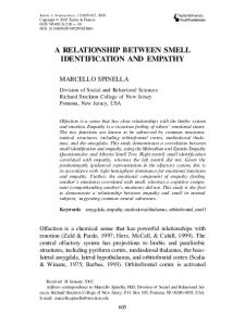
Second, as is illustrated in Figure 1, the trend in amphetamine

hospitalizations in California is non-linear over the extended period from 1993 to 1999. However, within the two time periods we examine, the trends leading up to the shock windows are roughly linear, which facilitates our identification strategy described below. We estimate the following interrupted time-series model to determine the effects of the supply shocks on methamphetamine consumption in California: (

)

(1)

4

These include the Methamphetamine Antiproliferation Act of 2000 and the Combat Methamphetamine Epidemic Act of 2005.

11

where At is the monthly number of amphetamine related hospitalizations, our measure of amphetamine use; shock;

is an indicator variable representing the period of the relevant supply

is a linear time trend; and

is the interaction between the shock

and trend variables, which we rescale to start at one at the beginning of the shock period. In this specification,

measures any level change in the dependent variable during the shock

period, and

measures any change in the trend of the dependent variable during

the shock period. Next, we estimate a similar interrupted time-series model to analyze the effects of the supply shock on risky sexual behavior in California: ( )

(2)

where St is the monthly number of syphilis diagnoses, our measure of risky sexual behavior, and all other variables are as defined above. Following the STI literature (e.g. Chesson, Harrison and Kassler 2000; Dee 2008; Francis and Mialon 2010), we also run specifications including a lagged dependent variable to account for the communicable nature of STIs. In addition to the California analysis, we use quarterly STI diagnosis rates collected by the CDC as a measure of risky sexual behavior for all 50 states and the District of Columbia.5 We estimate models similar to Equation (2), specifically: ( where

)

(3)

represents risky sexual behavior for state

at time ,

represent state fixed effects,

and all other variables are defined as above. When examining the 1995 shock window, we use the logged syphilis diagnosis rate for each state as our measure of risky sexual behavior. In the later time period surrounding the 1998 shock window, we have access to the number of

5

Monthly diagnoses are not available at the state level until after the end date of our shock periods.

12

chlamydia and gonorrhea diagnoses at the state and quarter level, so we also run models using these logged STI diagnosis rates as dependent variables. Each model is weighted by state population, and we adjust our standard errors to be robust to heteroskedasticity of an unknown form, including a within-state cluster correlation (Bertrand, Duflo and Mullainathan 2004). In this state panel setup, including a lagged dependent variable could lead to biased coefficients, as the lagged dependent variable is correlated with the mean of the dependent variable (Anderson and Hsiao 1982; Arellano and Bond 1991). Thus, in panel specifications including a lagged dependent variable we estimate GMM dynamic panel data models derived in Arellano and Bond (1991).

5. RESULTS 5.1. Summary Statistics Table 1 provides summary statistics for our samples.

The top two panels provide

statistics for the California sample, and the bottom two panels provide statistics for the U.S. states sample.

The numbers of observations in the California sample are 60 and 36,

corresponding to monthly observations over 5 and 3 years, respectively. During the analysis period for the 1995 shock window, the average number of primary syphilis diagnoses in each month is about 179, slightly higher among men (97) than among women (82). The monthly number of amphetamine-related hospitalizations is much higher at about 1,550 each month, and again the number is slightly higher for men than women. Mean amphetamine hospitalizations are only slightly lower, but syphilis diagnoses are about half as prevalent, during the analysis period for the 1998 shock window.

13

The numbers of observations in the U.S. states samples are 1020 and 612, corresponding to quarterly observations over 5 years and 3 years, respectively, for the 50 states and DC. The syphilis diagnosis rate in each quarter is about 0.55 per 100,000 people, also higher among men (0.84) than among women (0.26). As in California, syphilis is rarer during the analysis period for the 1998 supply shock window. However, we do have access to quarterly gonorrhea and chlamydia diagnoses over this period. While gonorrhea diagnosis rates are roughly equal at 31 per 100,000 people for men and women, the aggregate chlamydia diagnosis rate of 55 per 100,000 people masks rates that are four times as prevalent among women (88 per 100,000) as among men (19 per 100,000).

5.2. California Results We preview our California regression results by showing some suggestive graphical evidence. Figure 1 shows the trends of amphetamine-related hospitalizations and diagnoses of primary syphilis for California from 1993 to 1999. The line marked with +’s tracks amphetamine-related hospital admissions, and the line marked with x’s tracks primary syphilis diagnoses. The dashed, vertical, lines mark the August 1995 to September 1996 and the April 1998 to March 1999 methamphetamine supply shock windows. During the four months after July 1995, the start of the first supply shock window, amphetamine-related hospital admissions for both men and women dropped to less than 50 percent of their July 1995 value. By October 1996, the end of the first shock window, amphetamine-related hospitalizations had rebounded to roughly 75 percent of their pre-shock value for men and women combined and 70 percent of their pre-shock value for women. However, during the first shock window, syphilis diagnoses were relatively unchanged, continuing a slow trend downward that began in the early 1990s. Throughout the

14

second supply shock window, amphetamine hospitalizations fell by roughly 35 percent, but did not fully recover to their pre-shock-window levels thereafter. Notably, syphilis diagnoses continued their long-term downward trend before, during, and after the second shock window. Next, we show regression estimates of the effects of the supply shock windows on methamphetamine consumption in California. Table 2 displays these results, with the top panel displaying results for the 1995 shock window and the bottom panel displaying results for the 1998 shock window. We estimate models akin to Equation (1) in the left panel of Table 2. Pvalues from alternate Durbin-Watson tests, shown in the last row, suggest the presence of autocorrelation in our data. Thus, the right half of the table shows regressions including a lagged dependent variable. Similar to previous studies, we find that the 1995 supply shock window reduced amphetamine hospitalizations by about 17 percent.

The positive values of the

interaction coefficients suggest that the largest effect of the supply shock window happened in the first few months of the window, and this is borne out by Figure 1. The effects of the 1998 shock window are smaller, leading to a 10 percent decrease in amphetamine hospitalizations. The lack of significance of the interaction terms indicates that, unlike the 1995 shock window, the 1998 shock window resulted in a longer-lasting decrease in methamphetamine use. We turn now to estimating the effects of these supply shocks on risky sexual behavior in California, as proxied by syphilis diagnoses. In Figures 2 and 3, we show the graphical results of the models in Equation (2) for the two supply shock periods. The graphs show the total number, the number of male, and the number of female syphilis diagnoses along with the predictions generated from the interrupted time series regressions estimated for California at the month level. As the results indicate, there was little impact of either supply shock on syphilis diagnoses.

15

Tables 3 and 4 show our main results from estimating these regressions. Although most alternate Durbin-Watson statistics suggest that autocorrelation is not a problem, we include the lagged log number of syphilis diagnoses of the same gender in the second panel. In the last panel, we include the lagged log number of syphilis diagnoses of the opposite gender. As the symptoms for syphilis develop within 10 to 21 days, there may be a one month lag between changes in amphetamine consumption and changes in syphilis diagnoses. Therefore, we also estimate models with a one month lag between the dependent variable and the independent variables. These models are shown in the right-hand side columns of Tables 3 and 4. We estimate base models akin to Equation (2) for the 1995 supply shock in the top panel of Table 3. The coefficients for the shock window are either statistically insignificant or positive and statistically significant, as in some of the female specifications. The interaction terms, testing for differences in the trend of syphilis diagnoses during the shock period, are all very small and not statistically significant at conventional levels.6 In Table 4, we show results for the 1998 supply shock window. Unlike in Table 3, many of the coefficients for the initial effect of the shock are large, positive, and statistically significant, although these coefficients lose much of their statistical significance when syphilis diagnoses are forwarded by one month in the right half of the table. In addition to the initial positive effects of the supply shock, many of the interaction terms are negative and statistically significant. Since we rescale the interaction term to begin at a value of one in the first month of the shock period, the total effect of the shock 6

We tested the robustness of our results to variations in the 1995 shock period. Dobkin and Nicosia (2009) find that the price effects of the supply shock lasted only four months (August 1995 to November 1995) while amphetamine hospital admissions were affected for 18 months (August 1995 to January 1997). Additionally, Cunningham and Finlay (2012) empirically estimate the start and end dates for the 1995 shock as September 1995 to February 1996. Thus, we re-estimated the models in Tables 2 and 3 using these different time periods for the shock window. We find that the August 1995 to January 1997 and the September 1995 to February 1996 shock windows both led to large, statistically significant decreases in amphetamine hospitalizations, while the August 1995 to November 1995 shock window was not associated with reductions in amphetamine hospitalizations. Moreover, neither the August 1995 to January 1997 nor the September 1995 to February 1996 shock windows were associated with reductions in syphilis diagnoses. These results are available upon request.

16

during each month is given by the shock period coefficient plus the number of months since the shock period started multiplied by the interaction coefficient. Thus, the supply shock led to an initial increase in syphilis diagnoses followed by a downward trend in syphilis diagnoses.

5.3. State-Level Analysis Figure 4 shows some suggestive graphical evidence similar to that in Figures 2 and 3 for the effects of the 1995 supply shock measured at the national level. The figure shows total, male, and female syphilis diagnoses in the United States along with predictions generated from national-level interrupted time series regressions estimated at the quarterly level. The dashed, vertical, black lines mark the third quarter of 1995 to the third quarter of 1996 as the methamphetamine supply shock period. As the results indicate, there was little impact of the supply shock on syphilis diagnoses.

Table 5 shows our main results from estimating the

regressions in Equation Error! Reference source not found. for the 1995 supply shock and has the same general structure as Tables 3 and 4. The top part of the table shows models without any lagged STIs included as independent variables, the middle panel shows results from an ArellanoBond GMM model, and the bottom panel shows models adding in the lagged log rate of opposite sex STIs as an independent variable.7 In Table 5, the dependent variable is the logged syphilis diagnosis rate per 100,000 people, so the coefficients can be interpreted as semi-elasticities.8

7

The bias introduced by the lagged dependent variable decreases as the number of time periods increases, and as we have 20 periods in our data, the bias is likely to be small. Additionally, the Arellano-bond GMM utilizes increasingly many instruments in models with many time periods, raising concerns about over-identification (Roodman 2009). Thus, we also estimate a fixed effects OLS model including a lagged dependent variable. These results, available upon request, are very similar to the Arellano-Bond GMM models in that the coefficients corresponding to the shock period are small and not statistically significant. 8 Some states experience no syphilis diagnoses in a quarter, so we add one to each state’s number of syphilis diagnoses before computing our logged syphilis diagnosis rate. Given a relatively large number of zero diagnoses, we re-estimate our models using a fixed effects negative binomial model. These results, available upon request, are very similar to the OLS and dynamic panel results in that the 1995 supply shock did not have a negative effect on syphilis diagnoses, and in some cases had an initially positive effect on syphilis diagnoses.

17

The coefficients on the shock period are mostly positive, but not statistically significant, while the interaction terms, testing for differences in the trend of syphilis diagnoses during the shock period, are smaller, negative, and also not statistically significant. Finally, we examine the effect of the 1998 shock period on syphilis, gonorrhea, and chlamydia diagnoses at the state and quarter level. Figure 5 shows the actual and predicted United States syphilis diagnoses, where the prediction is generated from national-level interrupted time series regressions estimated at the quarterly level, and Table 6 shows results for regressions estimating Equation (3) and has the same structure as Table 5. In Figure 5, syphilis diagnoses are steadily decreasing before, during, and after the shock period, though the shock period appears to lead to an initial decrease in syphilis diagnoses in the national level prediction. However, when we estimate the model using our state-level data we find that the 1998 shock period generally did not lead to statistically significant changes in syphilis diagnoses.9 As syphilis diagnoses are increasingly rare in the late 1990s, our graphical results and regression results could be underpowered. An advantage of examining the 1998 supply shock period is the availability of additional diagnosis information for chlamydia and gonorrhea, much more common STIs.

Figure 6 shows actual and predicted United States chlamydia and

gonorrhea diagnoses during the 1998 supply shock period, and Tables 7 and 8 show regression results for logged gonorrhea rates and logged chlamydia rates. As is evident in Figure 6, both gonorrhea and chlamydia diagnoses continue on a steady upward trend before, during, and after the supply shock. In Tables 7 and 8, the 1998 supply shock window is associated with a small and statistically significant increase in gonorrhea and chlamydia diagnoses. Some specifications

9

Here again, we also estimate our models using a fixed effects negative binomial model, with results indicating no statistically significant negative effects of the 1998 supply shock window on syphilis diagnoses.

18

also show marginally statistically significant negative interaction terms, consistent with an initial increase in STI transmissions followed by a decrease back to the initial trend before the shock.10

6. CONCLUSION In this paper, we attempt to estimate the causal relationship between methamphetamine use and risky sexual behavior and STIs. To identify a causal relationship, we focus on large supply shocks to the methamphetamine market that occurred in May 1995 and October 1997. In our first set of results, we focus on the state of California since data on amphetamine-related hospital admissions and syphilis diagnoses are available at the monthly level for California and the methamphetamine epidemic was concentrated in the Western United States and particularly in California over the period we analyze (SAMHSA 2004). Using an interrupted time series approach, we find evidence that the supply shocks significantly reduced methamphetamine use, but no evidence that they reduced syphilis diagnoses. In additional analysis, we use state-level quarterly data on syphilis, gonorrhea, and chlamydia diagnoses, and again, we find no evidence that the shocks reduced diagnoses of STIs. Interestingly, we find some evidence, albeit evidence that is not strongly robust, that the 1995 shock was initially associated with an increase in syphilis among women in California and that the 1997 shock was initially associated with increases in gonorrhea and chlamydia in women across states. One possible explanation is that the higher methamphetamine prices following the shocks led some women to trade sex for drugs. Medical and epidemiologic research has long associated drug use, especially crack cocaine, with prostitution (Marx et al. 1991; Sterk 1999;

10

Here again we also estimate fixed effects OLS models including a lagged dependent variable. These results, available upon request, are also very similar to the Arellano-Bond GMM models in that the coefficients corresponding to the shock period are either small and not statistically significant or positive and statistically significant in the case of gonorrhea.

19

2000). As noted earlier, previous medical research estimates that heterosexual women who use methamphetamine are 6.7 times more likely to have received money or drugs for sex than heterosexual women who do not use methamphetamine (Molitor et al. 1998). Semple et al. (2011) report that 31 percent of females enrolled in a sexual risk reduction intervention in San Diego traded sex for methamphetamine in the past two months, while (Cheng et al. 2009) report that 34 percent of female methamphetamine users in San Diego have ever traded methamphetamine for sex. Other studies find that between 15 and 22 percent of women methamphetamine users recently exchanged sex for money (Semple, Grant and Patterson 2004). Moreover, methamphetamine use is very high among female sex workers (Patterson et al. 2006; Rusch et al. 2010; Kang et al. 2011). Examining this possible association is an interesting avenue for future research. One concern is that our estimates of the effects of the methamphetamine supply shocks on syphilis may be under-powered because syphilis diagnoses are not sufficiently common in the mid-to-late 1990s. However, the coefficients and standard errors in Tables 3-6 suggest that large decreases in syphilis diagnoses over the shock periods are highly unlikely. Also, while syphilis diagnoses were steadily declining during the 1990s, gonorrhea and chlamydia rates were steadily rising. The differing trends suggest that these three types of STIs measure different aspects of risky sexual behavior, and our analysis indicates that none were negatively associated with the supply shocks. It is also possible that while no negative relationship between methamphetamine and risky sexual behavior existed during the mid-to-late 1990s, a negative relationship developed more recently. However, medical and public health literature studying methamphetamine use and risky sexual behavior consistently found a negative correlation between the two in the mid-

20

to-late 1990s (Molitor et al. 1998; Molitor et al. 1999; Halkitis, Parsons and Stirratt 2001; Koblin et al. 2003a; Thiede et al. 2003; Colfax et al. 2004). Over the past decade, many states have enacted laws restricting methamphetamine precursors, and these laws may provide another source of exogenous variation in methamphetamine use. Unfortunately, however, there is little evidence suggesting that these more recent supply interdictions have been effective in reducing methamphetamine consumption (Dobkin, Nicosia and Weinberg 2013). Our results suggest that policies to reduce methamphetamine use may not reduce the prevalence of STIs. This is troubling, as methamphetamine use is increasingly targeted as a means of decreasing STIs among gay and bisexual men and other high-risk populations. Efforts to reduce STIs may be better centered around other policies, such as those that increase access to health care, increase screening of at-risk populations, help to find and treat partners of infected persons, and provide information on sexual health.

21

References Anderson, D. M. (2010). "Does information matter? The effect of the Meth Project on meth use among youths." Journal of Health Economics 29(5): 732-742. Anderson, T. W. and C. Hsiao (1982). "Formulation and estimation of dynamic models using panel data." Journal of Econometrics 18(1): 47-82. Arellano, M. and S. Bond (1991). "Some tests of specification for panel data: Monte Carlo evidence and an application to employment equations." Review of Economic Studies 58(2): 277-297. Bacchetti, P. and A. R. Moss (1989). "Incubation period of AIDS in San Francisco." Nature 338(6212): 251-253. Bertrand, M., E. Duflo and S. Mullainathan (2004). "How much should we trust differences-indifferences estimates?" Quarterly Journal of Economics 119(1): 249-275. Brewer, D. D., M. R. Golden and H. H. Handsfield (2006). "Unsafe sexual behavior and correlates of risk in a probability sample of men who have sex with men in the era of highly active antiretroviral therapy." Sexually Transmitted Diseases 33(4): 250-255. Cave, D. (2012). "Mexico Seizes Record Amount of Methamphetamine." New York Times, February 9, 2012. Retrieved November, 2013, from http://www.nytimes.com/2012/02/10/world/americas/mexico-seizes-15-tons-ofmethamphetamine.html. Centers for Disease Control and Prevention (2001). "Outbreak of syphilis among men who have sex with men--Southern California, 2000." Morbidity and Mortality Weekly Report 50(7): 117-120. Centers for Disease Control and Prevention. (2007). "Methamphetamine use and risk for HIV/AIDS." from http://www.cdc.gov/hiv/resources/factsheets/meth.htm. Centers for Disease Control and Prevention (2011). Sexually transmitted disease surveillance 2010. Atlanta, U.S. Department of Health and Human Services. Centers for Disease Control and Prevention. (2013a). "Chlamydia - CDC Fact Sheet." Retrieved 11/06/2013, from http://www.cdc.gov/std/chlamydia/STDFact-Chlamydia.htm. Centers for Disease Control and Prevention. (2013b). "Gonorreah - CDC Fact Sheet." Retrieved 11/06/2013, from http://www.cdc.gov/std/gonorrhea/stdfact-gonorrhea.htm. Cheng, W. S., et al. (2009). "Differences in sexual risk behaviors among male and female HIVseronegative heterosexual methamphetamine users." American Journal of Drug and Alcohol Abuse 35(5): 295-300.

22

Chesson, H., P. Harrison and W. J. Kassler (2000). "Sex under the influence: The effect of alcohol policy on sexually transmitted disease rates in the United States." Journal of Law and Economics 43(1): 215-238. Colfax, G., et al. (2004). "Substance use and sexual risk: a participant- and episode-level analysis among a cohort of men who have sex with men." American Journal of Epidemiology 159(10): 1002-1012. Corsi, K. F. and R. E. Booth (2008). "HIV sex risk behaviors among heterosexual methamphetamine users: literature review from 2000 to present." Current Drug Abuse Reviews 1(3): 292-296. Cunningham, J. K. and L. M. Liu (2003). "Impacts of federal ephedrine and pseudoephedrine regulations on methamphetamine-related hospital admissions." Addiction 98(9): 12291237. Cunningham, S. and K. Finlay (2012). "Parental substance abuse and foster care: Evidence from two methamphetamine supply shocks." Economic Inquiry 51(1): 764-782. Dee, T. S. (2008). "Forsaking all others? The effects of same-sex partnership laws on risky sex." Economic Journal 118(530): 1055-1078. Dobkin, C. and N. Nicosia (2009). "The war on drugs: methamphetamine, public health, and crime." American Economic Review 99(1): 324-349. Dobkin, C., N. Nicosia and M. Weinberg (2013). "Are supply-side drug control efforts effective? Evaluating OTC regulations targeting methamphetamine precursors." Working Paper: 152. Elifson, K. W., H. Klein and C. E. Sterk (2006). "Predictors of sexual risk-taking among new drug users." Journal of Sex Research 43(4): 318-327. Francis, A. M. and H. M. Mialon (2010). "Tolerance and HIV." Journal of Health Economics 29(2): 250-267. Gonzales, R., L. Mooney and R. A. Rawson (2010). "The methamphetamine problem in the United States." Annual Review of Public Health 31: 385-398. Gonzalez Castro, F., et al. (2000). "Cocaine and methamphetamine: differential addiction rates." Psychology of Addictive Behaviors 14(4): 390-396. Grossman, M., R. Kaestner and S. Markowitz (2004). "Get high and get stupid: The effect of alcohol and marijuana use on teen sexual behavior." Review of Economics of the Household 2(4): 413-441.

23

Grossman, M. and S. Markowitz (2005). "I did what last night?! Adolescent risky sexual behaviors and substance use." Eastern Economic Journal 31(3): 383-405. Halkitis, P. N., J. T. Parsons and M. J. Stirratt (2001). "A double epidemic: crystal methamphetamine drug use in relation to HIV transmission among gay men." Journal of Homosexuality 41(2): 17-35. Handsfield, H. H. and J. Schwebke (1990). "Trends in sexually transmitted diseases in homosexually active men in King County, Washington, 1980-1990." Sexually Transmitted Diseases 17(4): 211-215. Hser, Y. I., et al. (2008). "Contrasting trajectories of heroin, cocaine, and methamphetamine use." Journal of Addictive Diseases 27(3): 13-21. Hunt, D., S. Kuck and L. Truitt (2006). Methamphetamine use: lessons learned. Cambridge, MA, National Institute of Justice. Kang, D., et al. (2011). "Commercial sex venues, syphilis and methamphetamine use among female sex workers." AIDS Care 23 Suppl 1: 26-36. Koblin, B. A., et al. (2003a). "High-risk behaviors among men who have sex with men in 6 US cities: baseline data from the EXPLORE Study." American Journal of Public Health 93(6): 926-932. Koblin, B. A., et al. (2003b). "High-risk behaviors among men who have sex with men in 6 US cities: baseline data from the EXPLORE Study." American Journal of Public Health 93(6): 926-932. Lakdawalla, D., N. Sood and D. Goldman (2006). "HIV breakthroughs and risky sexual behavior." Quarterly Journal of Economics 121(3): 1063-1102. Levine, W. C., et al. (1998). "Increase in endocervical CD4 lymphocytes among women with nonulcerative sexually transmitted diseases." Journal of Infectious Diseases 177(1): 167174. Mansergh, G., et al. (2006). "Methamphetamine and sildenafil (Viagra) use are linked to unprotected receptive and insertive anal sex, respectively, in a sample of men who have sex with men." Sexually Transmitted Infections 82(2): 131-134. Marx, R., et al. (1991). "Crack, sex, and STD." Sexually Transmitted Diseases 18(2): 92-101. McBride, D., et al. (2008). The Relationship between state methamphetamine precursor laws and trends in small toxic lab (STL) seizures. Washington, DC, U.S. Department of Justice.

24

Molitor, F., et al. (1999). "Methamphetamine use and sexual and injection risk behaviors among out-of-treatment injection drug users." American Journal of Drug and Alcohol Abuse 25(3): 475-493. Molitor, F., et al. (1998). "Association of methamphetamine use during sex with risky sexual behaviors and HIV infection among non-injection drug users." Western Journal of Medicine 168(2): 93-97. Nonnemaker, J., M. Engelen and D. Shive (2011). "Are methamphetamine precursor control laws effective tools to fight the methamphetamine epidemic?" Health Economics 20(5): 519-531. Office of National Drug Policy Control (2001). What America's users spend on illegal drugs: 1988–2000. Washington, DC, Executive Office of the President. Patterson, T. L., et al. (2006). "Comparison of sexual and drug use behaviors between female sex workers in Tijuana and Ciudad Juarez, Mexico." Substance Use and Misuse 41(10-12): 1535-1549. Rawson, R. A., et al. (2002). "Drugs and sexual effects: role of drug type and gender." Journal of Substance Abuse Treatment 22(2): 103-108. Rolfs, R. T., et al. (1997). "A randomized trial of enhanced therapy for early syphilis in patients with and without human immunodeficiency virus infection. The Syphilis and HIV Study Group." New England Journal of Medicine 337(5): 307-314. Roodman, D. (2009). "How to do xtabond2: An introduction to difference and system GMM in Stata." Stata Journal 9(1): 86. Rusch, M. L., et al. (2010). "Distribution of sexually transmitted diseases and risk factors by work locations among female sex workers in Tijuana, Mexico." Sexually Transmitted Diseases 37(10): 608-614. SAMHSA (2004). NSDUH 2002-2004 sample based prevalence estimates, Office of Applied Studies. Semple, S. J., I. Grant and T. L. Patterson (2004). "Female methamphetamine users: social characteristics and sexual risk behavior." Women and Health 40(3): 35-50. Semple, S. J., et al. (2011). "Correlates of trading sex for methamphetamine in a sample of HIVnegative heterosexual methamphetamine users." Journal of Psychoactive Drugs 43(2): 79-88. Shoptaw, S. and C. J. Reback (2007). "Methamphetamine use and infectious disease-related behaviors in men who have sex with men: implications for interventions." Addiction 102 Suppl 1: 130-135.

25

Spinola, S. M., et al. (1996). "Haemophilus ducreyi elicits a cutaneous infiltrate of CD4 cells during experimental human infection." Journal of Infectious Diseases 173(2): 394-402. Sterk, C. E. (1999). Fast lives: women who use crack cocaine. Philadelphia, PA, Temple University Press. Sterk, C. E. (2000). Tricking and tripping: prostitution in the era of AIDS. Putnam Valley, NY, Social Change Press. Subcommittee on Crime of the Committee of the Judiciary (1995). Rising scourge of methamphetamine in America, House of Representatives, 104th Congress, First Session. Taylor, M. M., et al. (2007). "Methamphetamine use and sexual risk behaviours among men who have sex with men diagnosed with early syphilis in Los Angeles County." International Journal of STD and AIDS 18(2): 93-97. Thiede, H., et al. (2003). "Regional patterns and correlates of substance use among young men who have sex with men in 7 US urban areas." American Journal of Public Health 93(11): 1915-1921. U.S. v. Prather (2000). 205 F.3d 1265, United States Court of Appeals, Eleventh Circuit. United States Drug Enforcement Agency (1997). Temporary Exemption From Chemical Registration for Distributors of Pseudoephedrine and Phenylpropanolamine Products. F. Register. 62: 53959-53960. Wong, W., et al. (2005). "Risk factors for early syphilis among gay and bisexual men seen in an STD clinic: San Francisco, 2002-2003." Sexually Transmitted Diseases 32(7): 458-463.

26

Figure 1 Syphilis Diagnoses and Meth-Related Hospital Admissions California 1993 to 1999

01/93

300 100 200 Cases of Syphilis Meth Admissions Syphilis Diagnoses

0

Meth-Related Hosp. Admits 0 500 1000 1500 2000

Total

01/94

01/95

01/96

01/97

01/98

01/99

01/00

01/98

01/99

01/00

01/98

01/99

01/00

Month & Year

01/93

200 50 100 150 Cases of Syphilis

Meth Admissions Syphilis Diagnoses

0

Meth-Related Hosp. Admits 0 500 1000

Males

01/94

01/95

01/96

01/97

01/93

50 100 Cases of Syphilis

150

Females

Meth Admissions Syphilis Diagnoses

0

Meth-Related Hosp. Admits 0 500 1000

Month & Year

01/94

01/95

01/96

01/97

Month & Year

Notes: Data from the California Department of Public Health and the California Office of Statewide Health Planning and Development. The lines marked with +'s represent the total number of amphetamine-related hospital admissions in California in each month, and the lines marked with x's represent the total number of syphilis diagnoses in California in each month. The vertical dashed lines mark August 1995 to September 1996 and April 1998 to March 1999, the time periods of the supply shocks.

27

Figure 2 Actual and Predicted Syphilis Diagnoses California 1993 to 1997

0

Syphilis Diagnoses 50 100 150 200 250 300

Total

01/94

01/95 01/96 Month & Year

01/97

01/98

01/97

01/98

01/97

01/98

Males

0

Syphilis Diagnoses 50 100 150

200

01/93

01/93

01/94

01/95 01/96 Month & Year

0

Syphilis Diagnoses 50 100

150

Females

01/93

01/94

01/95 01/96 Month & Year

Notes: Data from the California Department of Public Health. The lines marked with x's represent the number of syphilis diagnoses in California in each month, and the unmarked lines represent the predicted number of syphilis diagnoses from a regression of logged syphilis counts on a linear time trend, an indicator variable for the period of the amphetamine supply shock, an interaction term between the time trend and shock period, quarterly fixed effects, and a constant. The vertical dashed lines mark August 1995 to September 1996, the time period of the supply shock.

28

Figure 3 Actual and Predicted Syphilis Diagnoses California 1997 to 1999

0

Syphilis Diagnoses 50 100

150

Total

01/97

01/98

01/99

01/00

01/99

01/00

01/99

01/00

Month & Year

0

Syphilis Diagnoses 20 40 60

80

Males

01/97

01/98 Month & Year

0

10

Syphilis Diagnoses 20 30 40 50

60

Females

01/97

01/98 Month & Year

Notes: Data from the California Department of Public Health. The lines marked with x's represent the number of syphilis diagnoses in California in each month, and the unmarked lines represent the predicted number of syphilis diagnoses from a regression of logged syphilis counts on a linear time trend, an indicator variable for the period of the amphetamine supply shock, an interaction term between the time trend and shock period, quarterly fixed effects, and a constant. The vertical dashed lines mark April 1998 to March 1999, the time period of the second supply shock.

29

Figure 4 Actual and Predicted Syphilis Diagnoses United States 1993 to 1997

0

Cases of Syphilis 1000 2000

3000

Total

93-1

94-1

95-1 96-1 Year & Quarter

97-1

98-1

97-1

98-1

97-1

98-1

0

Cases of Syphilis 500 1000 1500

2000

Males

94-1

95-1 96-1 Year & Quarter

Females

0

Cases of Syphilis 200 400 600

800

93-1

93-1

94-1

95-1 96-1 Year & Quarter

Notes: Data from the National Center for Health Statistics. The lines marked with x's represent the total number of syphilis diagnoses in the United States in each quarter, and the unmarked lines represent the predicted number of syphilis diagnoses from a regression of logged syphilis counts on a linear time trend, an indicator variable for the period of the amphetamine supply shock, an interaction term between the time trend and shock period, quarterly fixed effects, and a constant. The vertical dashed lines mark August 1995 to September 1996, the time period of the supply shock.

30

Figure 5 Actual and Predicted Syphilis Diagnoses United States 1997 to 1999

0

Cases of Syphilis 600 200 400

800

Total

97-1

98-1

99-1

00-1

99-1

00-1

99-1

00-1

Year & Quarter

0

Cases of Syphilis 200 400

600

Males

97-1

98-1 Year & Quarter

0

Cases of Syphilis 50 100 150

200

Females

97-1

98-1 Year & Quarter

Notes: Data from the National Center for Health Statistics. The lines marked with x's represent the total number of syphilis diagnoses in the United States in each quarter, and the unmarked lines represent the predicted number of syphilis diagnoses from a regression of logged syphilis counts on a linear time trend, an indicator variable for the period of the amphetamine supply shock, an interaction term between the time trend and shock period, quarterly fixed effects, and a constant. The vertical dashed lines mark April 1998 to March 1999, the time period of the second supply shock.

31

Figure 6 Actual and Predicted Gonorrhea and Chlamydia Diagnoses United States 1997 to 1999

100000

Gonorrhea

Chlamydia

98-1

99-1

00-1

97-1

Year & Quarter

Males

Males

Cases of Gonorrhea 20000 40000

99-1

00-1

99-1

00-1

99-1

00-1

0

0 97-1

98-1

Year & Quarter

Cases of Chlamydia 10000 20000 30000

60000

97-1

Total

0

0

Cases of Gonorrhea 50000

Cases of Chlamydia 50000 100000 150000 200000

Total

98-1

99-1

00-1

97-1

98-1

Year & Quarter

Year & Quarter

150000

Females

97-1

0

0

Cases of Chlamydia 50000 100000

Cases of Gonorrhea

50000

Females

98-1

99-1

00-1

97-1

Year & Quarter

98-1 Year & Quarter

Notes: Data from the National Center for Health Statistics. The lines marked with x's represent the total number of STI diagnoses in the United States in each quarter, and the unmarked lines represent the predicted number of STI diagnoses from a regression of logged STI counts on linear time trend, an indicator variable for the period of the amphetamine supply shock, an interaction term between the time trend and shock period, quarterly fixed effects, and a constant. The vertical dashed lines mark April 1998 to March 1999, the time period of the second supply shock.

32

Table 1 Summary Statistics Total Mean

Std. Dev

Mean

Males Std. Dev

Females Mean Std. Dev

California Sample 1993 to 1997 Syphilis Diagnoses Amphetamine Hospitalizations N

179.10 1553.00 60

62.60 311.20

97.10 823.20 60

32.30 166.20

82.00 729.80 60

31.40 149.40

California Sample 1997 to 1999 Syphilis Diagnoses Amphetamine Hospitalizations N

92.30 1481.40 36

23.10 254.00

51.70 792.20 36

13.40 137.50

40.60 689.20 36

11.60 120.80

State Level Sample 1993 to 1997 Syphilis Rate N

0.54 1020

0.91

0.84 1020

1.42

0.26 1020

0.46

State Level Sample 1997 to 1999 Syphilis Rate Gonorrhea Rate Chlamydia Rate N

0.23 31.51 54.69 612

0.27 20.32 17.75

0.36 31.93 19.41 612

0.42 22.34 7.70

0.10 30.97 88.26 612

0.14 18.96 29.28

Notes: Data from the California Department of Public Health, the California Office of Statewide Health Planning and Development, the U.S. Census, and the National Center for Health Statistics.

33

Table 2 Interrupted Time Series Regression Results of Effects of Methamphetamine Supply Shocks on Amphetamine Hospitalizations in California

1995 Shock Shock 95: 8/95-9/96 Shock x Trend Linear Trend N Adjusted R-Squared Durbin P-Value 1997 Shock Shock 98: 4/98-3/99 Shock x Trend Linear Trend N Adjusted R-Squared Durbin P-Value

Total

Base Model Male

Female

Including Lagged Dependent Variable Total Male Female

-0.208 ** (0.086) -0.003 (0.011) 0.007 *** (0.001) 60 0.44 0.00

-0.229 ** (0.086) -0.002 (0.012) 0.007 *** (0.001) 60 0.45 0.00

-0.183 * (0.087) -0.005 (0.011) 0.007 *** (0.001) 60 0.41 0.00

-0.171 *** (0.050) 0.016 *** (0.006) 0.001 (0.001) 60 0.83 n/a

-0.177 *** (0.056) 0.015 ** (0.006) 0.001 (0.001) 60 0.78 n/a

-0.169 *** (0.048) 0.014 ** (0.006) 0.001 (0.001) 60 0.79 n/a

-0.099 * (0.052) -0.006 (0.009) -0.011 *** (0.001) 36 0.77 0.03

-0.121 ** (0.051) -0.006 (0.010) -0.010 *** (0.001) 36 0.76 0.09

-0.075 (0.058) -0.006 (0.010) -0.012 *** (0.001) 36 0.73 0.02

-0.101 *** (0.029) 0.007 (0.006) -0.003 (0.002) 36 0.90 n/a

-0.121 *** (0.037) 0.006 (0.008) -0.005 ** (0.002) 36 0.83 n/a

-0.077 ** (0.035) 0.005 (0.008) -0.003 (0.002) 36 0.87 n/a

Notes: Data from the California Department of Public Health. The dependent variable in all specifications is the logged number of amphetamine hospitalizations. Coefficients represent semi-elasticities, and coefficients pertaining to indicator variables are transformed by exp(β)-1. Standard errors, shown in parentheses, are calculated from a robust variance-covariance matrix. In addition to the coefficients shown, all models include quarter fixed effects. The Lagged Dependent Variable regressions also include the lagged logged number of amphetamine hospitalizations as a regressor. Stars denote statistical significance: * Significant at 10%; ** significant at 5%; *** significant at 1%.

34

Table 3 Interrupted Time Series Regression Results of Effects of Methamphetamine Supply Shock on Syphilis Transmission in California Using August 1995 to September 1996 Shock Window

No Lagged Syphilis Shock 95: 8/95-9/96 Shock x Trend Linear Trend N Adjusted R-Squared Durbin P-Value Same Sex Lagged Syphilis Shock 95: 8/95-9/96 Shock x Trend Linear Trend N Adjusted R-Squared

Total

Base Model Male

Female

Total

0.049 (0.042) 0.000 (0.004) -0.018 *** (0.001) 60 0.88 0.5043

-0.005 (0.057) 0.002 (0.006) -0.017 *** (0.001) 60 0.85 0.87

0.114 ** (0.058) -0.002 (0.006) -0.02 *** (0.001) 60 0.83 0.5043

0.032 (0.051) 0.003 (0.004) -0.018 *** (0.001) 60 0.90 0.6544

-0.028 (0.060) 0.007 (0.007) -0.017 *** (0.001) 60 0.87 0.1656

0.103 (0.079) -0.001 (0.007) -0.02 *** (0.001) 60 0.84 0.8278

0.040 (0.044) 0.000 (0.004) -0.014 *** (0.004) 60 0.89

-0.005 (0.057) 0.002 (0.006) -0.016 *** (0.003) 60 0.85

0.103 * (0.061) -0.002 (0.006) -0.016 *** (0.004) 60 0.84

0.027 (0.049) 0.003 (0.004) -0.016 *** (0.004) 60 0.90

-0.028 (0.061) 0.007 (0.007) -0.018 *** (0.003) 60 0.87

0.094 (0.082) -0.001 (0.007) -0.018 *** (0.004) 60 0.84

-0.021 (0.065) 0.002 (0.007) -0.011 *** (0.003) 60 0.87

0.112 * (0.060) -0.002 (0.006) -0.017 *** (0.004) 60 0.83

-0.047 (0.060) 0.008 (0.007) -0.013 *** (0.003) 60 0.87

0.103 (0.079) -0.001 (0.007) -0.019 *** (0.004) 60 0.84

Opposite Sex Lagged Syphilis Shock 95: 8/95-9/96 Shock x Trend Linear Trend N Adjusted R-Squared

Forwarded by One Month Male Female

Notes: Data from the California Department of Public Health. The dependent variable in all specifications is the logged number of syphilis diagnoses. Coefficients represent semi-elasticities, and coefficients pertaining to indicator variables are transformed by exp(β)-1. Standard errors, shown in parentheses, are calculated from a robust variance-covariance matrix. In addition to the coefficients shown, all models include quarter fixed effects. The lagged syphilis regressions also include the lagged logged number of syphilis diagnoses (either same gender or opposite gender) as a regressor. Stars denote statistical significance: * Significant at 10%; ** significant at 5%; *** significant at 1%.

35

Table 4 Interrupted Time Series Regression Results of Effects of Methamphetamine Supply Shock on Syphilis Transmission in California Using April 1998 to March 1999 Shock Window

No Lagged Syphilis Shock 98: 4/98-3/99 Shock x Trend Linear Trend N Adjusted R-Squared Durbin P-Value Same Sex Lagged Syphilis Shock 98: 4/98-3/99 Shock x Trend Linear Trend N Adjusted R-Squared

Total

Base Model Male

Female

Total

0.208 ** (0.102) -0.038 ** (0.016) -0.015 *** (0.003) 36 0.61 0.09

0.131 (0.125) -0.031 (0.019) -0.015 *** (0.004) 36 0.49 0.06

0.309 ** (0.142) -0.045 ** (0.019) -0.017 *** (0.004) 36 0.56 0.22

0.127 (0.102) -0.030 ** (0.013) -0.013 *** (0.003) 36 0.67 0.31

0.129 (0.135) -0.031 (0.018) -0.013 *** (0.004) 36 0.45 0.39

0.128 (0.112) -0.028 ** (0.014) -0.015 *** (0.003) 36 0.74 0.45

0.282 ** (0.145) -0.046 ** (0.020) -0.020 *** (0.005) 36 0.62

0.211 (0.157) -0.041 * (0.023) -0.022 *** (0.004) 36 0.52

0.325 ** (0.172) -0.047 ** (0.021) -0.018 *** (0.005) 36 0.54

0.145 (0.122) -0.033 * (0.018) -0.015 *** (0.003) 36 0.66

0.154 (0.154) -0.036 (0.023) -0.016 *** (0.004) 36 0.45

0.109 (0.122) -0.026 * (0.015) -0.014 *** (0.003) 36 0.74

0.155 (0.171) -0.034 (0.026) -0.016 *** (0.005) 36 0.48

0.306 ** (0.148) -0.045 ** (0.018) -0.017 *** (0.006) 36 0.54

0.123 (0.154) -0.030 (0.022) -0.013 *** (0.004) 36 0.43

0.127 (0.113) -0.028 * (0.014) -0.015 *** (0.004) 36 0.73

Opposite Sex Lagged Syphilis Shock 98: 4/98-3/99 Shock x Trend Linear Trend N Adjusted R-Squared

Forwarded by One Month Male Female

Notes: Data from the California Department of Public Health. The dependent variable in all specifications is the logged number of syphilis diagnoses. Coefficients represent semi-elasticities, and coefficients pertaining to indicator variables are transformed by exp(β)-1. Standard errors, shown in parentheses, are calculated from a robust variance-covariance matrix. In addition to the coefficients shown, all models include quarter fixed effects. The lagged syphilis regressions also include the lagged logged number of syphilis diagnoses (either same gender or opposite gender) as a regressor. Stars denote statistical significance: * Significant at 10%; ** significant at 5%; *** significant at 1%.

36

Table 5 State-Level OLS and Dynamic Panel Data Regression Results of Effects of Methamphetamine Supply Shock on Syphilis Transmission Using Q3 1995 to Q2 1996 Shock Window Total

Base Model Male

Female

Total

0.042 (0.087) -0.016 (0.022) -0.080 *** (0.008) 1020 0.56

0.064 (0.103) -0.023 (0.026) -0.078 *** (0.008) 1020 0.53

0.057 (0.092) 0.002 (0.026) -0.076 *** (0.010) 1020 0.47

0.035 (0.067) -0.019 (0.018) -0.077 *** (0.008) 1020 0.55

0.043 (0.072) -0.025 (0.021) -0.074 *** (0.007) 1020 0.52

0.119 (0.083) -0.022 (0.024) -0.074 *** (0.010) 1020 0.46

Dynamic Panel Data Model Shock 95: Q3/95-Q2/96 -0.101 (0.059) Shock x Trend 0.018 (0.018) Linear Trend -0.043 *** (0.013) N 1020 ABond Z-Stat (1) -3.13 ABond Z-Stat (2) 1.52 Num Inst. 26

-0.049 (0.074) 0.006 (0.019) -0.046 *** (0.013) 1020 -2.61 0.52 26

-0.077 (0.061) 0.021 (0.020) -0.042 *** (0.016) 1020 -2.17 0.97 26

-0.027 (0.074) 0.010 (0.020) -0.037 *** (0.013) 1020 -2.94 1.42 26

0.022 (0.078) -0.005 (0.021) -0.042 *** (0.013) 1020 -2.59 0.53 26

0.016 (0.088) 0.004 (0.023) -0.037 ** (0.017) 1020 -2.31 1.21 26

0.055 (0.100) -0.023 (0.026) -0.052 *** (0.007) 1020 0.60

0.057 (0.096) 0.001 (0.027) -0.045 *** (0.006) 1020 0.53

0.026 (0.065) -0.026 (0.020) -0.050 *** (0.008) 1020 0.58

0.092 (0.086) -0.012 (0.026) -0.043 *** (0.006) 1020 0.53

No Lagged Syphilis Shock 95: Q3/95-Q2/96 Shock x Trend Linear Trend N R-Squared

Opposite-Sex Lagged Syphilis Shock 95: Q3/95-Q2/96 Shock x Trend Linear Trend N R-Squared

Forwarded by One Month Male Female

Notes: Data from the National Center for Health Statistics and the U.S. Census. The dependent variable in all specifications is the logged rate of syphilis diagnoses per 100,000 people. Coefficients represent semi-elasticities, and coefficients pertaining to indicator variables are transformed by exp(β)-1. Standard errors, shown in parentheses, are clustered at the state level, except in the dynamic panel data model, where they are calculated from a robust variance-covariance matrix. In addition to the coefficients shown, all models include state and quarter fixed effects. The Base Model and Opposite Sex Lagged STI regressions are weighted by state population, while the Dynamic Panel Data regressions are estimated using an Arrelano-Bond dynamic panel data model with one lag of the dependent variable and are not weighted by state population. Stars denote statistical significance: * Significant at 10%; ** significant at 5%; *** significant at 1%.

37

Table 6 State-Level OLS and Dynamic Panel Data Regression Results of Effects of Methamphetamine Supply Shock on Syphilis Transmission Using Q2 1998 to Q1 1999 Shock Window

No Lagged Syphilis Shock 98: Q2/98-Q1/99 Shock x Trend Linear Trend Num Adjusted R-Squared Dynamic Panel Data Shock 98: Q2/98-Q1/99 Shock x Trend Linear Trend N ABond Z-Stat (1) ABond Z-Stat (2) Num Inst

Total

Base Model Male

Female

Total

-0.047 (0.07) 0.017 (0.03) -0.030 *** (0.01) 612 0.06

-0.025 (0.09) 0.003 (0.03) -0.025 ** (0.01) 612 0.04

-0.019 (0.13) 0.022 (0.04) -0.032 ** (0.01) 612 0.04

0.080 (0.12) -0.038 (0.03) -0.027 *** (0.01) 612 0.09

0.089 (0.15) -0.050 (0.04) -0.020 * (0.01) 612 0.07

0.113 (0.17) -0.022 (0.05) -0.030 ** (0.01) 612 0.04

0.010 (0.10) 0.010 (0.04) -0.024 *** (0.01) 510 -4.951 1.652 16

0.017 (0.10) -0.008 (0.04) -0.019 ** (0.01) 510 -4.895 0.594 16

-0.084 (0.07) 0.048 * (0.03) -0.024 ** (0.01) 510 -4.873 0.043 16

0.173 * (0.10) -0.057 (0.03) -0.024 *** (0.01) 561 -5.211 2.051 16

0.231 ** (0.12) -0.082 ** (0.04) -0.018 ** (0.01) 561 -5.262 0.86 16

0.025 (0.09) -0.001 (0.03) -0.022 ** (0.01) 561 -4.622 -0.39 16

-0.008 (0.09) -0.005 (0.03) -0.021 ** (0.01) 561 0.06

-0.03 (0.14) 0.029 (0.05) -0.024 (0.02) 561 0.04

0.091 (0.16) -0.052 (0.04) -0.017 * (0.01) 612 0.08

0.118 (0.17) -0.022 (0.05) -0.026 * (0.01) 612 0.06

Opposite-Sex Lagged Syphilis Shock 98: Q2/98-Q1/99 Shock x Trend Linear Trend Num Adjusted R-Squared

Forwarded by One Month Male Female

Notes: Data from the National Center for Health Statistics and the U.S. Census. The dependent variable in all specifications is the logged rate of syphilis diagnoses per 100,000 people. Coefficients represent semi-elasticities, and coefficients pertaining to indicator variables are transformed by exp(β)-1. Standard errors, shown in parentheses, are clustered at the state level. In addition to the coefficients shown, all models include state and quarter fixed effects. The Base Model and Opposite Sex Lagged STI regressions are weighted by state population, while the Dynamic Panel Data regressions are estimated using an Arrelano-Bond dynamic panel data model with one lag of the dependent variable and are not weighted by state population. Stars denote statistical significance: * Significant at 10%; ** significant at 5%; *** significant at 1%.

38

Table 7 State-Level OLS and Dynamic Panel Data Regression Results of Effects of Methamphetamine Supply Shock on Gonorrhea Transmission Using Q2 1998 to Q1 1999 Shock Window

No Lagged Gonorrhea Shock 98: Q2/98-Q1/99 Shock x Trend Linear Trend Num Adjusted R-Squared Dynamic Panel Data Shock 98: Q2/98-Q1/99 Shock x Trend Linear Trend N

Total

Base Model Male

Female

Total

0.037 (0.03) -0.002 (0.01) 0.007 ** (0.00) 612 0.27

0.041 (0.04) -0.005 (0.01) 0.007 ** (0.00) 612 0.28

0.030 (0.04) 0.002 (0.01) 0.006 * (0.00) 612 0.20

0.086 ** (0.04) -0.021 (0.01) 0.007 ** (0.00) 612 0.26

0.087 ** (0.04) -0.026 * (0.02) 0.008 ** (0.00) 612 0.25

0.088 ** (0.04) -0.017 (0.01) 0.005 (0.00) 612 0.21

0.047 (0.04) -0.004 (0.02) 0.003 (0.00) 510

0.000 (0.07) 0.016 (0.03) 0.000 (0.00) 510

0.073 * (0.04) -0.015 (0.01) 0.003 (0.00) 510

0.122 *** (0.04) -0.035 ** (0.01) 0.002 (0.00) 561

0.139 *** (0.05) -0.043 *** (0.01) 0.003 (0.00) 561

0.118 *** (0.05) -0.031 * (0.02) 0.002 (0.00) 561

0.045 (0.04) -0.007 (0.01) 0.007 ** (0.00) 561 0.26

0.026 (0.04) 0.004 (0.01) 0.006 * (0.00) 561 0.21

0.085 ** (0.04) -0.027 * (0.01) 0.007 ** (0.00) 612 0.26

0.085 ** (0.04) -0.016 (0.01) 0.005 (0.00) 612 0.21

Opposite-Sex Lagged Gonorrhea Shock 98: Q2/98-Q1/99 Shock x Trend Linear Trend Num Adjusted R-Squared

Forwarded by One Month Male Female

Notes: Data from the National Center for Health Statistics and the U.S. Census. The dependent variable in all specifications is the logged rate of gonorrhea diagnoses per 100,000 people. Coefficients represent semi-elasticities, and coefficients pertaining to indicator variables are transformed by exp(β)-1. Standard errors, shown in parentheses, are clustered at the state level. In addition to the coefficients shown, all models include state and quarter fixed effects. The Base Model and Opposite Sex Lagged STI regressions are weighted by state population, while the Dynamic Panel Data regressions are estimated using an Arrelano-Bond dynamic panel data model with one lag of the dependent variable and are not weighted by state population. Stars denote statistical significance: * Significant at 10%; ** significant at 5%; *** significant at 1%.

39

Table 8 State-Level OLS and Dynamic Panel Data Regression Results of Effects of Methamphetamine Supply Shock on Chlamydia Transmission Using Q2 1998 to Q1 1999 Shock Window Total No Lagged Chlamydia Shock 98: Q2/98-Q1/99 Shock x Trend Linear Trend Num Adjusted R-Squared Dynamic Panel Data Shock 98: Q2/98-Q1/99 Shock x Trend Linear Trend N

Linear Trend Num Adjusted R-Squared

Female

Total

Forwarded by One Month Male Female

0.000 (0.03) 0.012 (0.01) 0.020 *** (0.00) 612 0.32

-0.023 (0.04) 0.020 (0.02) 0.034 *** (0.01) 612 0.34

0.000 (0.03) 0.011 (0.01) 0.017 *** (0.00) 612 0.27

0.052 * (0.03) -0.006 (0.01) 0.018 *** (0.00) 612 0.25

0.041 (0.05) -0.004 (0.02) 0.032 *** (0.00) 612 0.27

0.051 * (0.03) -0.005 (0.01) 0.016 *** (0.00) 612 0.21

0.043 (0.03) -0.005 (0.01) 0.020 *** (0.00) 510

-0.002 (0.07) 0.002 (0.02) 0.020 *** (0.01) 510

0.041 (0.03) -0.003 (0.01) 0.018 *** (0.00) 510

0.073 ** (0.03) -0.016 (0.01) 0.020 *** (0.00) 561

0.074 ** (0.04) -0.019 (0.01) 0.027 *** (0.00) 561

0.076 ** (0.03) -0.016 (0.01) 0.018 *** (0.00) 561

-0.005 (0.04) 0.009 (0.02) 0.030 *** (0.01) 561 0.27

-0.002 (0.04) 0.012 (0.01) 0.016 *** (0.00) 561 0.22

0.041 (0.04) -0.005 (0.01) 0.030 *** (0.00) 612 0.28

0.051 * (0.03) -0.005 (0.01) 0.016 *** (0.00) 612 0.21

Opposite-Sex Lagged Chlamydia Shock 98: Q2/98-Q1/99 Shock x Trend

Base Model Male

Notes: Data from the National Center for Health Statistics and the U.S. Census. The dependent variable in all specifications is the logged rate of chlamydia diagnoses per 100,000 people. Coefficients represent semi-elasticities, and coefficients pertaining to indicator variables are transformed by exp(β)-1. Standard errors, shown in parentheses, are clustered at the state level. In addition to the coefficients shown, all models include state and quarter fixed effects. The Base Model and Opposite Sex Lagged STI regressions are weighted by state population, while theDynamic Panel Data regressions are estimated using an Arrelano-Bond dynamic panel data model with one lag of the dependent variable and are not weighted by state population. Stars denote statistical significance: * Significant at 10%; ** significant at 5%; *** significant at 1%.

40