JOURNAL OF APPLIED PHYSICS 100, 104906 共2006兲

The scaling laws of transport properties for fractal-like tree networks Peng Xu and Boming Yua兲 Department of Physics, Huazhong University of Science and Technology, 1037 Luoyu Road, Wuhan 430074, People’s Republic of China

共Received 15 May 2006; accepted 11 September 2006; published online 27 November 2006兲 The scaling laws of transport properties are very important for understanding the transport mechanisms of the fractal-like tree networks, which have received extensive attention recently. In this paper, we analyze the transport properties including electrical conductivity, heat conduction, convective heat transfer, laminar flow, and turbulent flow in the networks and also derive the scaling exponents of the transport properties in the networks. We show that the scaling laws are different for different transport processes and the scaling exponents are sensitive to microstructures of the networks. The models and results we present here may shed light on the transport mechanisms of the networks such as the natural systems, nanotube networks, microelectronic cooling networks, organisms, fracture networks in oil/water reservoirs, seepage flow in porous networks/media, etc., and might provide guidance for design of composites with the tree structures. © 2006 American Institute of Physics. 关DOI: 10.1063/1.2392935兴 I. INTRODUCTION

The tree network structures arise extensively in circulatory systems of plants and mammals, communications, social cooperation networks, economic systems, river basins, oil/ water reservoirs, power supply systems of cities, microelectronic cooling systems, etc.1,2 The transport properties 共electrical, thermal, fluid flow, etc.兲 in the tree networks, the design, optimization, and application of the tree networks have received considerable attention recently.3–19 Since Murray’s law3 for cardiovascular system in 1926, various and numerous subsequent researches have focused on the investigation of the networks. Many researchers use this tree network model to explain the mechanisms of natural transports.7–9,12,15 Some others design and optimize the networks and apply the tree networks to various engineering fields such as oil/water reservoirs, power supply systems of a city, microelectronic cooling systems, etc. For example, Bejan and co-workers4–6 developed “constructal theory” by optimizing the access between one point and a finite volume. Cheng and Chen11 designed a rectangular shape fractal-tree nets fixed on the top and bottom of matrix wafer for the cooling of a microelectronic chip. Yu and Li19 investigated the effective thermal conductivity of composites with embedded self-similar H-shaped fractal-like tree networks. They found that the fractal-like tree networks play an important role and can significantly reduce the thermal conductivity. This structure might be applied for designing insulating or conducting structures such as space equipments. The self-similar fractal-tree network can be space filling,20 which has been shown significantly more error 共variability兲 tolerant than other structures and therefore has an evolutionary advantage.21 The scaling laws of transport properties of the fractal-like tree network are very important and may shed light on the natural network structures. a兲

Author to whom correspondence should be addressed; electronic mail: [email protected]

0021-8979/2006/100共10兲/104906/8/$23.00

Neuman22 showed that the hydraulic conductivity K⬘ in porous media scales with the support volume V by K⬘ ⬃ Va, where a is the scaling exponent and takes on specific value 1 / 2. Winter and Tartakovsky23 demonstrated that when a pore network in porous media can be represented by a collection of hierarchical trees, scalability of the pore geometry leads to the 1 / 2-power scaling law. While West et al.7–9 derived the allometric scaling law which is a quarter-power scaling law. Allometric laws are widely recognized as powerlaw relations between geometric and functional 共e.g., flow兲 parameters of living bodies. From a purely theoretical standpoint, Bejan24 found that the total heat current convected by a double tree is proportional to the total volume raised to power 3 / 4. In this paper, we focus on the transport properties of the fractal-like tree networks and study their scaling laws, including those of electrical conductivity, heat conduction, convective heat transfer, laminar flow, and turbulent flow. These might be useful for understanding the transport mechanisms of the tree structures such as the natural systems, nanotube networks, microelectronic cooling networks, organisms, fracture networks in oil/water reservoirs, seepage flow in porous networks/media, etc. II. FRACTAL-LIKE TREE NETWORK

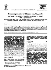
Figure 1 displays a typical self-similar tree structure and the kth branching level with n 共=2兲 branches. Since the present work deals with the self-similar tree networks with finite volume branches, there is a possible smallest element/ unit because the daughter branches may touch mother stems after finite repeats. Therefore, the structures in this paper are called fractal-like tree networks. If, however, the volume of all branches is neglected or stems are assumed to be infinitely thin, the self-similar tree structures are fractals.20 Generally speaking, the tree/branched network 共see Fig. 1兲 is composed of N branches from level 0 to levels m 共total number of branching levels兲. A typical branch with branching angle ␪ at some intermediate level k 共k = 0 , 1 , 2 , . . . , m兲

100, 104906-1

© 2006 American Institute of Physics

Downloaded 28 Nov 2006 to 211.67.26.127. Redistribution subject to AIP license or copyright, see http://jap.aip.org/jap/copyright.jsp

104906-2

J. Appl. Phys. 100, 104906 共2006兲

P. Xu and B. Yu m

m

k=0

k=0

V = 兺 NkVk = 兺 nk␲共dk/2兲2lk = Vmnm

1 − 共n␥␤2兲−共m+1兲 , 1 − 共n␥␤2兲−1 共3兲

where Vm is the volume of a terminal branching tube. Consequently, the dimensionless volume can be obtained by V+ =

1 − 共n␥␤2兲−共m+1兲 V = nm . 1 − 共n␥␤2兲−1 Vm

共4兲

In the following discussion, we follow the assumption by West et al.7 that the final branch of the network 共such as the capillary in the circulatory system兲 is a size-invariant unit. That is, the terminal units 共capillaries兲 are invariant and the parameters 共lm, dm, vm, ⌬pm, Rm, etc.兲 of the terminal branch are independent of body size. The fractal branching network presented here should be viewed as an idealized representation, in which we ignore complications such as tapering of vessels and nonlinear effects. These play only a minor role in determining the properties of the entire network and could be incorporated in more detailed analysis of specific systems. For convenience, we only consider the transports along the tubes of the network and neglect the transports in the matrix material.

III. ELECTRICAL CONDUCTIVITY FIG. 1. 共a兲 A typical self-similar tree structure 共Ref. 10兲, 共b兲 the kth branching level with n共=2兲 branches, and 共c兲 a fractal-like tree network.

has length lk and diameter dk, and each tube branches into nk smaller daughter branches at the next level. In order to characterize the architecture of the tree/branched network, we introduce scale factors ␥k ⬅ lk+1 / lk and ␤k ⬅ dk+1 / dk. In this paper, we focus on the tree/branched network with fractal characteristics; thus we shall invoke the selfsimilar fractal results by West et al.,7 i.e., ␥k = ␥, ␤k = ␤, and nk = n which are all independent of k. It is easy to get lk = l0␥k = lm␥k−m

and

dk = d0␤k = dm␤k−m ,

共1兲

where l0 and d0 are the length and diameter of the 0th branching level while lm and dm are the length and diameter of the terminal branching level. According to the fractal characteristics of the structure,20 we have n = ␥−Dl = ␤−Dd ,

In this section, we will derive the scaling law between the electrical conductivity and the volume of the network. The electrical resistance of a kth single tube is Rk = ␳lk / Ak = 4␳lk / ␲d2k , where ␳ is the resistivity of a material. The electrical resistance of the entire network is given by m

R=兺

k=0

共5兲

The effective resistivity of the network can be obtained m lk from ␳e = RAe / le, where the equivalent length le = 兺k=0 −共m+1兲 −1 = lm关1 − ␥ 兴 / 共1 − ␥ 兲, and the equivalent cross-sectional 2 / 4兲nm共1 area of the network is defined as Ae = V / le = 共␲dm −1 −共m+1兲 2 −共m+1兲 2 −1 兴关1 − 共n␥␤ 兲 兴 / 关1 − 共n␥␤ 兲 兴. Then − ␥ 兲 / 关1 − ␥ the effective resistivity of the network can be expressed as

␳e = ␳

共2兲

where Dl is the fractal dimension of tube length distribution, and Dd is the fractal dimension for diameter distribution 共also called diameter exponent兲. Fractal dimensions Dl and Dd are generally limited between 1 and 3, and the value Dd = 3 is an optimized result known as Murray’s law. Then, for n = 2, ␥ and ␤ are in the ranges of 0.5–0.7937. The total number of branches at level k is Nk = nk and the total number of branches of the whole network is N m Nk = 共1 − nm+1兲 / 共1 − n兲. For convenience, we assume = 兺k=0 that every branching tube is smooth cylinder. Therefore, the total volume of the network can be obtained as

m

4␳lk Rk Rm 1 − 共n␤2/␥兲m+1 =兺 = . Nk k=0 ␲nkd2k nm 1 − n␤2/␥

冋

1 − ␥−1 1 − ␥−共m+1兲

册

2

1 − 共n␥␤2兲−共m+1兲 1 − 共n␤2/␥兲m+1 . 1 − 共n␥␤2兲−1 1 − n ␤ 2/ ␥ 共6兲

The effective electrical conductivity 共EEC兲 of the network can be obtained as

␴e = =

1 ␳e

冋

1 1 − ␥−共m+1兲 ␳ 1 − ␥−1

册

2

1 − 共n␥␤2兲−1 1 − n ␤ 2/ ␥ . 2 −共m+1兲 1 − 共n␥␤ 兲 1 − 共n␤2/␥兲m+1 共7兲

The dimensionless EEC of the network is

Downloaded 28 Nov 2006 to 211.67.26.127. Redistribution subject to AIP license or copyright, see http://jap.aip.org/jap/copyright.jsp

104906-3

␴+ = =

J. Appl. Phys. 100, 104906 共2006兲

P. Xu and B. Yu

␴e ␴

冋

1 − ␥−共m+1兲 1 − ␥−1

册

2

1 − 共n␥␤2兲−1 1 − n ␤ 2/ ␥ , 共8兲 1 − 共n␥␤2兲−共m+1兲 1 − 共n␤2/␥兲m+1

where ␴ = 1 / ␳ is the electrical conductivity of material of the network. It can be clearly seen from Eqs. 共7兲 and 共8兲 that the EEC of the network is equal to the material electrical conductivity of the network at ␤ = n−1/2 共Dd = 2, area-preserving constraint兲, i.e., ␴e = ␴. Due to Eq. 共3兲 and n␥␤2 ⬍ 1, for m Ⰷ 1 the total volume V is approximately proportional to 共␥␤2兲−共m+1兲. As n␤2 / ␥ ⬎ 1, the total electrical resistance is approximately proportional to 共␤2 / ␥兲m+1, and the EEC is proportional to a constant. From Eqs. 共3兲 and 共5兲, we get ln共␤2/␥兲 ln R =− , ln V ln共␥␤2兲

共9兲

which means that the total electrical resistance R of the fractal branched network is proportional to Va, where the scaling exponent a = −ln共␤2 / ␥兲 / ln共␥␤2兲. According to Eq. 共2兲, the scaling exponent can also be expressed as a = 共Dd − 2Dl兲 / 共Dd + 2Dl兲. The employment of the volumepreserving 共space-filling fractal system ␥ = n−1/3兲 and areapreserving 共␤ = n−1/2兲 conditions7–9 from one generation to the next, which correspond to fractal dimensions Dl = 3 and Dd = 2, respectively, results in a = −1 / 2. Thus, the scaling law R ⬃ V−1/2 holds, which means that the −1 / 2-power scaling law exists between the electrical resistance and the volume under the volume- and area-preserving conditions. However, when n␤2 / ␥ ⬍ 1, the total electrical resistance is approximately proportional to 共1 / n兲m and the effective electrical conductivity is approximately proportional to 共n␤2 / ␥兲m+1. Therefore, − m ln n ln n ln R = 2 ⬵ ln V − 共m + 1兲ln共␥␤ 兲 ln共␥␤2兲 and

ln共n␤2/␥兲 ln ␴e =− . ln V ln共␥␤2兲

共10兲

Equation 共10兲 indicates that the electrical resistance and the EEC are proportional to Va and Vb, respectively, where the scaling exponents a = ln n / ln共␥␤2兲 and b = −ln共n␤2 / ␥兲 / ln共␥␤2兲. And the scaling exponents can also be and b = 共Dd − 2Dl written as a = −DlDd / 共Dd + 2Dl兲 + DlDd兲 / 共Dd + 2Dl兲. IV. HEAT CONDUCTION

With the increasing miniaturization of electronic equipments, a lot of investigations were involved in heat transfer in the tree networks.11,19,24,25 Xu et al.25 analyzed the heat conduction through “Y” shaped fractal-like tree networks and obtained the expression for thermal conductivity in the networks. The network is assumed to be composed of the material of high thermal conductivity ␭, which is much higher than that of the material around the channels. So, heat conduction along the channels is assumed and in other directions is neglected. This means that the one dimensional heat

flow model is applied. The total thermal resistance of the entire network can be obtained by the thermal-electrical analogy as25 m

R=兺

k=0

Rk Rm 1 − 共n␤2/␥兲m+1 = . N k n m 1 − n ␤ 2/ ␥

共11兲

And then the effective thermal conductivity 共ETC兲 is obtained by equating that of the network with an equivalent single tube as ␭e = ␭

冋

1 − ␥−共m+1兲 1 − ␥−1

册

2

1 − 共n␥␤2兲−1 1 − n ␤ 2/ ␥ . 1 − 共n␥␤2兲−共m+1兲 1 − 共n␤2/␥兲m+1 共12兲

The dimensionless ETC is written as ␭+ = =

␭e ␭

冋

1 − ␥−共m+1兲 1 − ␥−1

册

2

1 − 共n␥␤2兲−1 1 − n ␤ 2/ ␥ . 1 − 共n␥␤2兲−共m+1兲 1 − 共n␤2/␥兲m+1 共13兲

Equation 共13兲 shows that the ETC reaches its greatest value, which is equal to the thermal conductivity of the tube material at the area-preserving condition, i.e., ␤ = n−1/2 共Dd = 2兲. Compared with Eqs. 共8兲 and 共13兲, it is seen that the ETC and the EEC of the network have the same form, so the scaling law of the heat conduction is the same as that of electrical conductivity, and this is expected.

V. CONVECTIVE HEAT TRANSFER

The effective convective heat transfer coefficient of the whole fractal-like tree network is derived in this section. The flow through each tube is assumed to be laminar and fully developed both thermally and hydrodynamically, and the Nusselt number remains constant through each level of branches. Thus, the convective heat transfer coefficient of the higher-level branching will increase with hk+1 / hk = dk / dk+1 = 1 / ␤; consequently, hk = hm␤m−k .

共14兲

The heat flux through the network is assumed to be uniform and varies from one level to another. Therefore, a fully developed flow with constant heat flux in uniform cross section yields a constant temperature different ⌬T between the wall surface and bulk flow. Consequently, the total convective heat transfer rate is m

Q = 兺 NkhkSk⌬T = nmQm k=0

1 − 共n␥兲−共m+1兲 , 1 − 共n␥兲−1

共15兲

where Sk = ␲dklk is the heat transfer area at the kth branching level and Qm = hm␲dmlm⌬T is the convective heat transfer rate at the mth branching level. The total heat transfer area S of the network is given by

Downloaded 28 Nov 2006 to 211.67.26.127. Redistribution subject to AIP license or copyright, see http://jap.aip.org/jap/copyright.jsp

104906-4

J. Appl. Phys. 100, 104906 共2006兲

P. Xu and B. Yu m

m

S = 兺 N kS k = 兺 n k␲ d kl k = n mS m k=0

k=0

1 − 共n␥␤兲−共m+1兲 . 1 − 共n␥␤兲−1

共16兲

Then the effective convective heat transfer coefficient of the whole network can be calculated from he = Q / S⌬T, i.e., he = hm

1 − 共n␥兲−共m+1兲 1 − 共n␥␤兲−1 . 1 − 共n␥兲−1 1 − 共n␥␤兲−共m+1兲

共17兲

The dimensionless of he can be easily found to be h+ =

he 1 − 共n␥兲−共m+1兲 1 − 共n␥␤兲−1 = . hm 1 − 共n␥兲−1 1 − 共n␥␤兲−共m+1兲

共18兲

Generally, n␥ ⬎ 1 and m Ⰷ 1, then as n␥␤ ⬎ 1, he is approximately proportional to a constant. While as n␥␤ ⬍ 1, he and S are approximately proportional to 共n␥␤兲m+1 and 共␥␤兲−共m+1兲, respectively. Thus he is proportional to Sb⬘, where the scaling exponent b⬘ = −ln共n␥␤兲 / ln共␥␤兲. Because the total volume V is approximately proportional to 共␥␤2兲−共m+1兲 for n␥␤2 ⬍ 1 关see Eq. 共3兲兴, he is proportional to Vb, where the scaling exponent b = −ln共n␥␤兲 / ln共␥␤2兲. Due to Eq. 共2兲 the scaling exponents can also be expressed in terms of the fractal dimensions as b⬘ = DlDd / 共Dl + Dd兲 − 1 and b = 共DlDd − Dd − Dl兲 / 共Dd + 2Dl兲. VI. FLUID FLOW A. Laminar flow

Let us first consider the case of incompressible fully developed laminar flow. The viscous resistance for flow in a single tube is given by the Poiseuille formula Rk = 128 ␮lk / 共␲d4k 兲, where ␮ is the viscosity of fluid. Then the total flow resistance of the network can be expressed as m

R=兺

k=0

Rk Rm 1 − 共n␤4/␥兲m+1 = . N k n m 1 − n ␤ 4/ ␥

共19兲

Then, using the method applied in literatures,26,27 we can derive the effective permeability of the network

冋

Ke = Km nm

1 − 共1/␥兲m+1 1 − n␤4/␥ 1 − 1/␥ 1 − 共n␤4/␥兲m+1

册

1/2

1 , T

共20兲

where Km is the permeability of the mth branching level and T is the tortuosity of the network 共for example, T for the = 共1 − ␥m+1兲 / 兵共1 − ␥兲关1 + ␥共1 − ␥m兲cos ␪ / 共1 − ␥兲兴其 fractal-like tree network between one point and a straight line兲.26 The dimensionless form of the effective permeability can then be expressed as K+ =

冋

1 − 共1/␥兲m+1 1 − n␤4/␥ Ke = nm 1 − 1/␥ 1 − 共n␤4/␥兲m+1 Km

册

1/2

1 . T

共21兲

As m Ⰷ 1 and n␤4 / ␥ ⬍ 1, a good approximation to Eq. 共19兲 is R = Rm / 共1 − n␤4 / ␥兲nm, and because Rm is invariant, R ⬃ n−共m+1兲. But as n␤4 / ␥ ⬎ 1, R ⬃ 共␤4 / ␥兲m+1. The total volume V ⬃ 共␥␤2兲−共m+1兲 for n␥␤2 ⬍ 1. So, the total flow resistance of the network R is proportional to Va, where the scaling exponents a = ln n / ln共␥␤2兲 as n␤4 / ␥ ⬍ 1 and a = −ln共␤4 / ␥兲 / ln共␥␤2兲 as n␤4 / ␥ ⬎ 1. The scaling exponents can also be expressed as the functions of fractal dimensions,

a = −DlDd / 共Dd + 2Dl兲 and a = 共Dd − 4Dl兲 / 共Dd + 2Dl兲. West et al.7–9 obtained the famous allometric scaling law by assuming n␤4 / ␥ ⬍ 1 and gave the power law R ⬃ V−3/4 at the volume- and area-preserving limitations. Our result is consistent with the allometric scaling law as n␤4 / ␥ ⬍ 1. It has been shown26,27 that when m Ⰷ 1, the tortuosity T approaches different asymptotic values for different branching angles ␪. This implies that the tortuosity and the branching angle ␪ have no effect on the scaling law of permeability as m Ⰷ 1. As n␤4 / ␥ ⬍ 1 and m Ⰷ 1, the effective permeability of the network Ke is proportional to 共n / ␥兲共m+1兲/2, and as n␤4 / ␥ ⬎ 1 and m Ⰷ 1, Ke is proportional to ␤−2共m+1兲 关see Eq. 共20兲兴; while the total volume V is proportional to 共␥␤2兲−共m+1兲 for n␥␤2 ⬍ 1 关see Eq. 共3兲兴. Therefore, the scaling law of permeability with the support volume can be written as Ke ⬃ Vb ,

共22兲

where the scaling exponents b = −共1 / 2兲ln共n / ␥兲 / ln共␥␤2兲 as n␤4 / ␥ ⬍ 1 and b = 2 ln ␤ / ln共␥␤2兲 as n␤4 / ␥ ⬎ 1. The scaling exponents with fractal dimensions are b = 共1 / 2兲Dd共1 + Dl兲 / 共Dd + 2Dl兲 and b = 2Dl / 共Dd + 2Dl兲. It can be clearly seen that the scaling exponent b is independent of the branching angle ␪, i.e., although the permeability is strongly related to branching angle ␪, the scaling laws of the permeability are independent of the branching angle ␪ when m Ⰷ 1. According to the area-preserving relation the scaling exponent b = 1 / 2, i.e., Ke ⬃ V1/2, which is the same as that by Neuman22 and Winter and Tartakovsky.23 This means that the 1 / 2-power scaling law exists between the permeability and the volume under area-preserving condition. It is worth pointing out that our simple model yields the 1 / 2-power scaling law only under the area-preserving condition, whereas the same conductivity scaling arises under both the pore area and the pore length preserving conditions from one level to another in Winter and Tartakovsky’s complicated model with subtrees.23 B. Turbulent flow

For the fully rough turbulent flow, the pressure drop over a kth branching tube of mean velocity vk yields ⌬Pk = f

lk ␳v2k , dk 2

共23兲

where ␳ is the density of fluid and the Darcy friction factor f is essentially constant in the fully rough turbulent limit, which is independent of Reynolds number or flow rate. Since ˙ 2, the the pressure drop ⌬Pk is proportional to the flow rate m 28 flow resistance is Rk =

⌬Pk 8f lk = , ˙ 2 ␳␲2 d5k m

共24兲

˙ = ␳vkAk. The total flow resistance of the network can where m be written as m

R=兺

k=0

Rk Rm 1 − 共n2␤5/␥兲m+1 = . N2k n2m 1 − n2␤5/␥

共25兲

From the conservation of mass, we have

Downloaded 28 Nov 2006 to 211.67.26.127. Redistribution subject to AIP license or copyright, see http://jap.aip.org/jap/copyright.jsp

104906-5

J. Appl. Phys. 100, 104906 共2006兲

P. Xu and B. Yu

Q = n mv m␲

2 dm d2k = n kv k␲ , 4 4

共26兲

vk = vmnm−k␤2共m−k兲 .

共27兲

According to Eq. 共23兲 and with the aid of Eq. 共27兲, the total pressure drop of the network can be expressed as m

⌬P = 兺 ⌬Pk = k=0

␳ flmvm2 1 − 共n2␤5/␥兲m+1 1 − n 2␤ 5/ ␥ 2dm

共28a兲

1 − 共n2␤5/␥兲m+1 . 1 − n 2␤ 5/ ␥

共28b兲

The mean flow velocity of the network can be derived from Eq. 共27兲, m

v=

N kv kl k 兺 k=0

= vm

冒兺 m

N kl k

k−0

1 − 共␤2/␥兲m+1 1 − 共n␥兲−1 . 1 − ␤2/␥ 1 − 共n␥兲−共m+1兲

共29兲

The network can be equivalent to a single tube; thus, le ␳v2 , de 2

⌬P = f

共30兲

where the equivalent length le = lm关1 − ␥−共m+1兲兴 / 共1 − ␥−1兲, and de is the diameter of the equivalent single tube. Inserting Eqs. 共28兲 and 共29兲 into Eq. 共30兲 gives 1 − 共1/␥兲m+1 1 − n2␤5/␥ de = dm 1 − 1/␥ 1 − 共n2␤5/␥兲m+1 ⫻

冋

1 − 共␤2/␥兲m+1 1 − 共n␥兲−1 1 − ␤2/␥ 1 − 共n␥兲−共m+1兲

册

2

.

共31兲

Compared with the apparent Darcy law Q = 共K / ␮兲A共dP / dL兲, the effective permeability of the network for fully rough turbulent flow can be obtained by K e = n mK m ⫻

冋

1 − 1/␥ 1 − 共n2␤5/␥兲m+1 Ke = nm 1 − 共1/␥兲m+1 1 − n2␤5/␥ Km ⫻

and therefore

=⌬Pm

K+ =

1 − 1/␥ 1 − 共n2␤5/␥兲m+1 1 − 共1/␥兲m+1 1 − n2␤5/␥

1 − ␤2/␥ 1 − 共n␥兲−共m+1兲 1 − 共␤2/␥兲m+1 1 − 共n␥兲−1

册

4

,

共32兲

where Ke is the effective permeability of the network, and Km = 2␮dm / ␳ f vm is the permeability of the terminal single tube. In the above analysis, we have neglected the tortuousness of the network in derivation of the effective permeability. Usually the permeability is related to the tortuosity T.29,30 However, as discussed above, since the tortuosity T has no influence on the scaling exponent as m Ⰷ 1, T is assumed to be 1.0 for simplicity. The dimensionless effective permeability of the network can be easily obtained as

冋

1 − ␤2/␥ 1 − 共n␥兲−共m+1兲 1 − 共␤2/␥兲m+1 1 − 共n␥兲−1

册

4

.

共33兲

It can be clearly seen from Eqs. 共32兲 and 共33兲 that Ke = Km at m = 0 or n = 1 and ␤ = 1 共i.e., a single tube兲, and this is in accord with the practical situation. As m Ⰷ 1 and n2␤5 / ␥ ⬍ 1, a good approximation to Eq. 共25兲 is that the total flow resistance R of the network is proportional to n−2共m+1兲. But, as n2␤5 / ␥ ⬎ 1, R ⬃ 共␤5 / ␥兲m+1. While the total volume of the network is approximately proportional to 共␥␤2兲−共m+1兲 for n␥␤2 ⬍ 1. Therefore, R is proportional to Va, where the scaling exponents a = 2 ln n / ln共␥␤2兲 or a = −2DlDd / 共Dd + 2Dl兲 as n2␤5 / ␥ ⬍ 1 and a = −ln共␤5 / ␥兲 / ln共␥␤2兲 or a = 共Dd − 5Dl兲 / 共Dd + 2Dl兲 as n2␤5 / ␥ ⬎ 1. Thus, the network exhibits the −3 / 2 power law between flow resistance and volume at the volume-preserving and areapreserving conditions for fully rough turbulent flow, and this is different from the −3 / 4 power law for laminar flow. While for the effective permeability, since ␥ ⬍ 1, ␤2 / ␥ ⬍ 1, and n␥ ⬎ 1, generally, the effective permeability of the network Ke ⬃ 共n␥兲m+1 as n2␤5 / ␥ ⬍ 1. But as n2␤5 / ␥ ⬎ 1, Ke ⬃ 共n3␤5兲m+1. That means that the effective permeability of the network is proportional to Vb, where the scaling exponents b = −ln共n␥兲 / ln共␥␤2兲 as n2␤5 / ␥ ⬍ 1 and b = −ln共n3␤5兲 / ln共␥␤2兲 as n2␤5 / ␥ ⬎ 1. Invoking Eq. 共2兲 gives the exponents b = Dd共Dl − 1兲 / 共Dd + 2Dl兲 and b = 共3Dd − 5兲 / 共Dd + 2Dl兲, respectively. As ␥ = n−1/3 共space-filling fractal system兲 and ␤ = n−1/2 共area-preserving relation兲, Ke ⬃ V1/2 for turbulent flow, which is the same as that for laminar flow only under the area-preserving condition 共␤ = n−1/2兲. VII. RESULTS AND DISCUSSIONS

The scaling laws for different transport properties are summarized in Table I. The electrical conductivity and heat conduction in the fractal-like tree network have the same scaling law. That is, as n␤2 / ␥ ⬎ 1, the EEC 共or ETC兲 is proportional to a constant and the total resistance R ⬃ Va, where the scaling exponent a = −ln共␤2 / ␥兲 / ln共␥␤2兲. Under volumeand area-preserving relations, R ⬃ V−1/2. When n␤2 / ␥ ⬍ 1, the resistance and the EEC 共or ETC兲 are proportional to Va and Vb, respectively, where the scaling exponents a = ln n / ln共␥␤2兲 and b = −ln共n␤2 / ␥兲 / ln共␥␤2兲. For convective heat transfer, as n␥␤ ⬎ 1, he is proportional to a constant; as n␥␤ ⬍ 1, he is proportional to Sb⬘ and Vb, respectively, where the scaling exponents b⬘ = −ln共n␥␤兲 / ln共␥␤兲 and b = −ln共n␥␤兲 / ln共␥␤2兲. For the laminar fluid flow, the resistance and effective permeability scale with the support volume by R ⬃ Va and Ke ⬃ Vb, respectively. In the case of laminar flow, the scaling exponent between resistance and the volume is a = ln n / ln共␥␤2兲 as n␤4 / ␥ ⬍ 1 and is a = −ln共␤4 / ␥兲 / ln共␥␤2兲 as n␤4 / ␥ ⬎ 1. The −3 / 4 power law exists between the flow resistance and the volume under the volume- and areapreserving relations. This is consistent with the famous allometric scaling law presented by West et al.7 The scaling exponent between effective permeability and the volume is

Downloaded 28 Nov 2006 to 211.67.26.127. Redistribution subject to AIP license or copyright, see http://jap.aip.org/jap/copyright.jsp

104906-6

J. Appl. Phys. 100, 104906 共2006兲

P. Xu and B. Yu

TABLE I. Scaling laws for transport properties in the fractal branched networks. 关The scaling exponents can also be expressed by the fractal dimensions of the network as discussed above via Eq. 共2兲.兴 Electrical and heat conductivity n␤2 / ␥ ⬎ 1 R ⬃ Va ln共␤ / ␥兲 2

a=−

n␥␤ ⬎ 1

n␥␤ ⬍ 1

n␤4 / ␥ ⬍ 1

n␤4 / ␥ ⬎ 1

n 2␤ 5 / ␥ ⬍ 1

n 2␤ 5 / ␥ ⬎ 1

R ⬃ Va

he ⬃ C

he ⬃ Vb

R ⬃ Va

R ⬃ Va

R ⬃ Va

R ⬃ Va

ln n ln共␥␤2兲 ␴e ⬃ Vb

b=−

Turbulent flow

n␤2 / ␥ ⬍ 1

a=

ln共␥␤2兲 ␴e ⬃ C

Laminar flowa

Convective heat transfer

ln共n␤2 / ␥兲 ln共␥␤ 兲 2

b=−

ln共n␥␤兲

ln共␥␤2兲 h e ⬃ S b⬘

b⬘ = −

ln共n␥␤兲 ln共␥␤兲

ln n ln共r␤2兲 Ke ⬃ Vb

a=

b=−

ln共␤ / ␥兲 4

a=−

ln共␥␤2兲 Ke ⬃ Vb

ln共n / ␥兲 2 ln共␥␤ 兲 2

b=

2 ln ␤ ln共␥␤2兲

2 ln n ln共r␤2兲 Ke ⬃ Vb

a=

b=−

ln共n␥兲 ln共␥␤ 兲 2

a=−

ln共␤5 / ␥兲

ln共␥␤2兲 Ke ⬃ Vb

b=−

ln共n3␤5兲 ln共␥␤2兲

Our results R ⬃ V−3/4 at ␥ = n−1/3 and ␤ = n−1/2 is the same as the result of Ref. 7, Ke ⬃ V1/2 at ␤ = n−1/2 is consistent with the conclusion of Refs. 22 and 23.

a

b = −共1 / 2兲ln共n / ␥兲 / ln共␥␤2兲 as n␤4 / ␥ ⬍ 1 and is b = 2 ln ␤ / ln共␥␤2兲 as n␤4 / ␥ ⬎ 1. The relation Ke ⬃ V1/2 under the area-preserving condition 共␤ = n−1/2 or Dd = 2兲 is consistent with that by Winter and Tartakovsky.23 For the turbulent flow, the scaling exponents are different. The scaling exponents a = 2 ln n / ln共␥␤2兲 and b = −ln共n␥兲 / ln共␥␤2兲 as n2␤5 / ␥ ⬍ 1, a = −ln共␤5 / ␥兲 / ln共␥␤2兲 and b = −ln共n3␤5兲 / ln共␥␤2兲 as n2␤5 / ␥ ⬎ 1. The same power scaling law Ke ⬃ V1/2 is found under volume- and areapreserving conditions 共␥ = n−1/3, ␤ = n−1/2兲. In addition, the scaling exponents can also be expressed in terms of fractal dimensions as discussed above. Generally, the total number of branching levels m Ⰷ 1 in the natural branched network 共for example, the bronchial tree of mammals has about 16 branching levels兲. So n = 2 and 10艋 m 艋 30 are employed for numerical calculations in this work. The results are shown in Figs. 2–5. Figure 2 shows the scaling laws of electrical conductivity and heat conduction at different length and diameter ratios. As shown in Fig. 2共a兲,

FIG. 2. The scaling laws at different length and diameter ratios: 共a兲 The electrical resistance vs the supporting volume R+ ⬃ 共V+兲a, and 共b兲 The electrical conductivity vs the support volume ␴+ ⬃ 共V+兲b.

the fitting constants a for the electrical resistance or the thermal resistance versus the supporting volume are −0.495 at ␥ = 2−1/3 and ␤ = 2−1/2, −0.165 at ␥ = 0.6 and ␤ = 0.7, and −0.362 at ␥ = 0.6 and ␤ = 0.5, respectively. While the scaling exponents a predicted by our model are −1 / 2, −0.165, and −0.365 at different microstructures. The predicted scaling exponents b between the EEC or ETC and the supporting volume are −0.096 and −0.193 at ␥ = 0.6 and ␤ = 0.5, and ␥ = 0.7 and ␤ = 0.5, while the fitting constants b = −0.099 and −0.193, respectively, see Fig. 2共b兲. Figure 3 indicates that the effective convective heat transfer coefficient he is proportional to Sb⬘ and Vb. The fitting constants are −0.316 and −0.211 for ␥ = ␤ = 0.6, −0.200 and −0.143 for ␥ = 0.6 and ␤ = 0.7, and −0.206 and −0.131 for ␥ = 0.7 and ␤ = 0.6; while the predicted scaling exponents b⬘ are −0.322, −0.201, and −0.201, and b are −0.214, −0.142, and −0.127, respectively. Figure 4 presents the scaling laws for laminar flow at ␥

FIG. 3. The scaling laws at different length and diameter ratios: 共a兲 The effective convective heat transfer coefficient vs the surface h+ ⬃ 共S+兲b⬘, and 共b兲 the effective convective heat transfer coefficient vs the supporting volume h+ ⬃ 共V+兲b.

Downloaded 28 Nov 2006 to 211.67.26.127. Redistribution subject to AIP license or copyright, see http://jap.aip.org/jap/copyright.jsp

104906-7

J. Appl. Phys. 100, 104906 共2006兲

P. Xu and B. Yu

FIG. 6. The scaling law between the effective permeability and the supporting volume K+ ⬃ 共V+兲b at ␥ = 2−1/3 and ␤ = 2−1/2 for 1 艋 m 艋 30, the fitting constants are b = 0.496 共⬇1 / 2兲 for laminar flow and b = 0.508 共⬇1 / 2兲 for turbulent flow.

FIG. 4. The scaling laws at different length and diameter ratios: 共a兲 The laminar flow resistance vs the supporting volume R+ ⬃ 共V+兲a, and 共b兲 the effective permeability vs the supporting volume K+ ⬃ 共V+兲b.

= 2−1/3 and ␤ = 2−1/2, ␥ = 2−1/3 and ␤ = 2−1, ␥ = 2−1 and ␤ = 2−1/3, and ␥ = 2−1/2 and ␤ = 2−1/3, respectively. The fitting constants for flow resistance and volume are a = −0.747共⬇−3 / 4兲, −0.429共⬇−3 / 7兲, −0.200共=−1 / 5兲, and −0.686共⬇−5 / 7兲, and those for effective permeability and volume are b = 0.499共⬇1 / 2兲, 0.287共⬇2 / 7兲, 0.3999共⬇2 / 5兲, and 0.554共⬇4 / 7兲, respectively. While the scaling exponents

predicted by our model are a = −3 / 4, −3 / 7, −1 / 5, and −5 / 7; b = 1 / 2, 2 / 7, 2 / 5, and 4 / 7, respectively. Figure 5 is for the case of turbulent flow, the fitting constants for flow resistance are a = −1.480 共⬇−3 / 2兲 at ␥ = 2−1/3 and ␤ = 2−1/2, a = −0.3999 共⬇−2 / 5兲 at ␥ = 2−1 and ␤ = 2−1/3, and a = −0.983 共⬇−1兲 at ␥ = 2−1/2 and ␤ = 2−1/3 关Fig. 5共a兲兴. While our predicted scaling exponents are a = −3 / 2, −2 / 5, and −1, respectively. Figure 5共b兲 indicates the scaling laws between the effective permeability for turbulent flow and the volume 共Ke ⬃ Vb兲 at different microstructures, and the fitting constants are b = 0.5095 共⬇1 / 2兲 at ␥ = 2−1/3 and ␤ = 2−1/2, b = 0.2842 共⬇2 / 7兲 at ␥ = 2−1/3 and ␤ = 2−1, and b = 1.0602 共⬇8 / 7兲 at ␥ = 2−1/2 and ␤ = 2−1/3, respectively. The predicted scaling exponents are b = 1 / 2, 2 / 7, and 8 / 7, respectively. It is evident from Figs. 2–5 that the scaling exponents depend on the microstructures and are very sensitive to the microstructures 共␥ , ␤兲. Note that the result of Ke ⬃ V1/2 under the volume- and area-preserving relations for laminar and turbulent flows is correct even for small m 共see Fig. 6兲. VIII. CONCLUDING REMARKS

We have derived and summarized the electrical conductivity, heat conduction, convective heat transfer, laminar flow and turbulent flow, as well as their scaling laws in the fractallike tree networks. It is shown that the scaling laws are different for different transport properties and are very sensitive to the microstructures of the networks. The models and results we present here may be helpful for understanding the transport properties in the network structures such as the natural systems, nanotube networks, microelectronic cooling networks, organisms, fractures in oil/water reservoirs, seepage flow in porous networks/media, etc., and might provide guidance for design of composites with tree structures. ACKNOWLEDGMENT

This work was supported by the National Natural Science Foundation of China through Grant No. 10572052. N. MacDonald, Tree and Networks in Biological Models 共Wiley, Chichester, 1983兲. 2 F. Cramer, Chaos and Order 共VCH-Weinheim, Germany, 1993兲. 3 C. D. Murray, Proc. Natl. Acad. Sci. U.S.A. 12, 207 共1926兲. 4 G. A. Ledezma, A. Bejan, and M. R. Errera, J. Appl. Phys. 82, 89 共1997兲. 1

FIG. 5. The scaling laws at different length and diameter ratios: 共a兲 The turbulent flow resistance vs the supporting volume R+ ⬃ 共V+兲a, and 共b兲 the effective permeability vs the supporting volume K+ ⬃ 共V+兲b.

Downloaded 28 Nov 2006 to 211.67.26.127. Redistribution subject to AIP license or copyright, see http://jap.aip.org/jap/copyright.jsp

104906-8

J. Appl. Phys. 100, 104906 共2006兲

P. Xu and B. Yu

M. Neagu and A. Bejan, J. Appl. Phys. 86, 1136 共1999兲. A. Bejan, Shape and Structure, From Engineering to Nature 共Cambridge University Press, Cambridge, UK, 2000兲. 7 G. B. West, J. H. Brown, and B. J. Enquist, Science 276, 122 共1997兲. 8 G. B. West, J. H. Brown, and B. J. Enquist, Nature 共London兲 400, 664 共1999兲. 9 J. H. Brown, G. B. West, and B. J. Enquist, Scaling in Biology 共Oxford University, Oxford, UK, 2000兲. 10 S. Bohn, B. Andreotti, S. Douady, J. Munzinger, and Y. Couder, Phys. Rev. E 65, 061914 共2002兲. 11 Y. P. Cheng and P. Chen, Int. J. Heat Mass Transfer 45, 2643 共2002兲. 12 K. A. McCulloh, J. S. Sperry, and F. R. Adler, Nature 共London兲 421, 939 共2003兲. 13 S. N. Dorogovtsev and J. F. F. Mendes, Evolution of Networks: From Biological Nets to the Internet and the WWW 共Oxford University, Oxford, 2003兲. 14 M. Durand, Phys. Rev. E 70, 046125 共2004兲. 15 B. Mauroy, M. Filoche, E. R. Weibel, and B. Sapoval, Nature 共London兲 427, 633 共2004兲. 16 S. M. Senn and D. Poulikakos, J. Appl. Phys. 96, 842 共2004兲.

L. Gosselin and A. Bejan, J. Appl. Phys. 98, 104903 共2005兲. M. Durand, Phys. Rev. E 73, 016116 共2006兲. 19 B. M. Yu and B. W. Li, Phys. Rev. E 73, 066302 共2006兲. 20 B. B. Mandelbrot, The Fractal Geometry of Nature 共Freeman, New York, 1982兲. 21 M. F. Shlesinger and B. J. West, Phys. Rev. Lett. 67, 2106 共1991兲. 22 S. P. Neuman, Geophys. Res. Lett. 21, 349 共1994兲. 23 C. L. Winter and D. M. Tartakovsky, Geophys. Res. Lett. 28, 4367 共2001兲. 24 A. Bejan, Int. J. Heat Mass Transfer 44, 699 共2001兲. 25 P. Xu, B. M. Yu, M. J. Yun, and M. Q. Zou, Int. J. Heat Mass Transfer 49, 3746 共2006兲. 26 P. Xu, B. M. Yu, Y. J. Feng, and Y. J. Liu, Physica A 369, 884 共2006兲. 27 P. Xu, B. M. Yu, Y. J. Feng, and M. Q. Zou, Phys. Fluids 18, 078103 共2006兲. 28 A. Bejan, L. A. O. Rocha, and S. Lorente, Int. J. Therm. Sci. 39, 949 共2000兲. 29 J. Bear, Dynamics of Fluid in Porous Media 共Elsevier, New York, 1972兲. 30 F. A. L. Dullien, Porous Media: Fluid Transport and Pore Structure 共Academic, New York, 1979兲.

5

17

6

18

Downloaded 28 Nov 2006 to 211.67.26.127. Redistribution subject to AIP license or copyright, see http://jap.aip.org/jap/copyright.jsp