The Spill-Over E¤ects of Con‡ict on Economic Growth in Neighbouring Countries in Africa Olaf J. de Groot Bocconi University and IEP This version: 13 November 2007

Abstract In this article, the in‡uence of con‡ict on the economies of neighbouring countries is discussed. The results from previous papers showed a strong negative e¤ect for an entire area around a country su¤ering from con‡ict, but this paper reaches a di¤erent conclusion. The paper uses more recent data and adjusts the methodology employed in previous papers. Additionally, a new type of contiguity matrix is constructed and used in the actual analysis. The …nal analysis consists of a large number of regressions and concludes that con‡ict actually has two opposing e¤ects. Firstly, like con‡ict countries themselves, directly contiguous countries actually su¤er from the negative e¤ects of proximate con‡ict. Secondly, however, there is also a positive spill-over of con‡ict which a¤ects non-contiguous countries and this e¤ect is larger for countries that are closer to the con‡ict country. The results from the paper predominantly hold for the most violent kind of con‡ict. Keywords: Con‡ict; Economic Growth; Spatial Econometrics; Africa JEL code: D74, O40

1

Introduction

Many have written about the in‡uence of con‡ict on economic growth. The conclusion is clear-cut: con‡ict is bad for growth in the short term1 (e.g. Collier, 1999 and Koubi, 2005). For long-run analyses, the phoenix e¤ect (Organski and Kugler, 1980) Address of the author: Olaf J. de Groot, Bocconi University, Via Sarfatti 25, 20136, Milan, Italy. e-mail: [email protected]. 1 It has long been hypothesised that the causality between growth and con‡ict runs both ways. In their excellent paper, Miguel et al. (2004) use an Instrumental Variable approach to show that negative growth shocks indeed increases the probability of con‡ict for a sample of African countries.

1

is occasionally cited as a reason why little evidence has been found that con‡ict negatively a¤ects growth. According to the theory of the phoenix factor, post-con‡ict nations actually grow faster than their peaceful counterparts. This appears to be a simple example of the conditional convergence theorem (Barro and Sala-i-Martin, 1992), which states that countries with a lower GDP, ceteris paribus, grow faster. After all, a country that has lost considerably from an episode of con‡ict has already proven to possess the potential ability for a certain amount of growth: it merely needs to recover its lost resources and enjoy the conditional convergence. Outside the …eld of economics, political scientists and others have performed substantial research on the actual spill-over e¤ects of con‡ict itself. They have addressed whether con‡ict is likely to spill over and what the external conditions are that make con‡ict more likely to infect proximate states (e.g. Sambanis, 2002). It seems reasonable to say that particular types of con‡ict are more likely to spill over, while other types of con‡ict are less likely to do so. In Africa, particularly, due to its colonial history, tribal con‡icts are relatively common. These tend to spill over easily, because particular tribes may be distributed over two or more countries. On the other hand, civil war that is caused by speci…c local conditions is much less likely to a¤ect the probability of con‡ict in neighbouring countries. The relationship between con‡ict in one country and economic growth in nearby countries, however, has not often been researched2 . One paper that addresses the in‡uence of regional political instability, de…ned as coups and revolutions, …nds a signi…cantly negative e¤ect for neighbouring countries (Ades and Chua, 1997). The only papers I am aware of that address the spill-over e¤ects of actual con‡ict on growth in contiguous countries are by Murdoch and Sandler (2002a, 2002b, 2004), who have researched exactly this topic. The results of Murdoch and Sandler are discussed in the following section, in which I also argue that an alternative speci…cation of the basic model may yield improved results. In the section that follows, a model is presented that o¤sets some of the shortcomings of Murdoch and Sandler. The data used in the analysis are presented in the fourth section and the results of the analysis can be found in the …fth section. The sixth and …nal section wraps up the …ndings and discusses some of the implications that result from the conclusions.

2

Literature overview

As mentioned earlier, Murdoch and Sandler have published a number of papers on this topic. All of their papers basically use the same model, which is an augmented Solow growth model, as was described by Mankiw et al. (1992). These latter authors 2

This does not imply that the role of spatial e¤ects itself is not often analysed. Research on the relationship between growth and geography is done thorougly in many di¤erent settings. Abreu et al. (2004) give a clear overview of the di¤erent econometric techniques used in the …eld

2

argued that Solow’s (1956) model was correct in its intentions, but disregarded the possibility that equilibrium growth resulted from increased human capital and only focused on physical capital and labour growth rates instead. Using the common production function with diminishing returns to scale for all inputs, Mankiw et al. set up a new model to be used for growth analysis. Murdoch and Sandler use this basic model and add a number of externalities which may also be able to in‡uence the growth rate. In their papers, they argue that domestic and adjacent con‡ict are two sources that may have a negative in‡uence on growth rates. While the authors assert that some of the problems caused by con‡ict work through the classical channels, by in‡uencing the levels of capital and labour growth, they add that there might be other, unobserved, channels through which con‡ict in‡uences growth. The di¤erent papers vary in time periods, the sample of countries and contiguity de…nitions and a clear evolution in the papers is visible. For each paper, the authors choose to analyse the data in both a long term style, creating a cross-section dataset, and a short term one, where a panel dataset can be used. In the latter case, the unit of observation is a 5-year period and most of the discussions of the results focus on these analyses. The long term regressions yield little in terms of concrete results, which is attributed to the phoenix e¤ect, as mentioned earlier. With regards to the country sample, two of Murdoch and Sandler’s papers (2002a and 2004) use worldwide samples, whereas the third paper (2002b) distinguishes di¤erent geographical regions and reports separate results for each of these regions. This paper is particularly interesting for the current analysis, because it is possible to make a direct comparison between the results they …nd for Africa and the results from the current paper. The de…nition of contiguity is one of the other things where the di¤erent papers distinguish themselves from each other. The …rst paper uses only direct contiguity, in which countries are required to actually share a border in order for them to be considered contiguous. The second paper, on the other hand, uses the Gleditsch and Ward (2001) dataset on minimal distances between nations to construct new types of contiguity matrices. While varying the maximum distance from 0 to 800 km in steps of 50 km, they use dummy variables to indicate whether a country is within a particular range. This provides the authors with 17 di¤erent contiguity matrices for each region and they report the results with the highest explanatory power. The third paper uses a similar method, but only for the minimum distances of 100, 300 and 800 km. In each paper, Murdoch and Sandler come to the conclusion that in the short run, civil con‡ict indeed has a negative e¤ect on economic growth in neighbouring countries. In the third paper, Murdoch and Sandler conclude that the e¤ect of con‡ict is felt over an 800 km minimal distance, while the 2002b paper concludes that di¤erent regions have di¤erent relevant minimal distances3 . 3

For Africa, 100 km minimal distance is the optimal distance, for Latin America it is 300 km or 0 km, depending on the de…nition of con‡ict, for Asia it is 600 km or 500 km and for the pooled

3

The papers by Murdoch and Sandler have signi…cant merit, as these are the …rst publications that address the issue of neighbouring countries su¤ering from the spillover e¤ects of con‡ict. However, a number of issues should be addressed in order to improve the results of these papers. First of all, there are some practical issues to be considered with regards to the data used by the authors. Some of the underlying datasets have recently been updated and extended beyond 19954 , some contain signi…cant errors and, occasionally, the coding of the data by Murdoch and Sandler seems to have been somewhat imprecise5 . In addition to the aforementioned data concerns, I would like to point out two theoretical improvements, which may strengthen the original results. The …rst point that is addressed in this paper is the rigidity of Murdoch and Sandler’s theoretical model with respect to the direction of the spill-over e¤ects. As a result of their model selection, the spill-over e¤ect is required to be unidimensional, while the following section of this paper will put forward a number of arguments in favour of a model in which two di¤erent types of contiguity matrices are to be used in a single regression. This adaptation leads to the possibility that some neighbours are in‡uenced positively, whereas others are in‡uenced negatively. This also leads to the second potential improvement of the theoretical model. The employment of a minimal distance dataset is an excellent idea, but by deciding to use dummy variables a lot of relevant information is lost. In order to encompass all possible information, a new type of contiguity matrix is introduced in order to deal with exactly this drawback.

3

Model

The basic model used in this paper is the same as the one used by Murdoch and Sandler in their papers. In summary, this is a basic Solow (1956) model, augmented in order to include human capital (Mankiw et al., 1992). As a result, the inputs for the Cobb Douglas production function are capital (K), labour (L) and human capital (H) and the function looks as follows: Y (t) = K(t) H(t) [A(t)L(t)]1

(1)

In this model and are the elasticities of output with respect to capital and human capital respectively and their sum is greater than 0, but less than 1. A(t) represents the exogenously determined e¤ectiveness of labour. The production function Latin American and Asian sample the optimal minimal distance is 700 km. 4 Particularly, Murdoch and Sandler use the Penn World Tables (PWT) 5.7, but it is now possible to use the more recent version PWT 6.2 (Heston et al., 2006) or the World Development Indicators (Worldbank, 2007). 5 When interpreting the dataset used for Murdoch and Sandler (2004), several examples can be found of data that are internally inconsistent.

4

in equation 1 displays constant returns to scale and diminishing marginal returns for all inputs and satis…es the Inada conditions. Thanks to the constant returns to scale, it is possible to express production in production per e¤ective worker, by dividing the left- and right-hand sides of equation 1 by AL: (2)

y(t) = k(t) h(t)

K H Y , k = AL and h = AL . where y = AL The next step is to transform equation 2 into an equation that shows how changes in the parameters in‡uence production. These so-called transition equations are derived in Mankiw et al. (1992) and look as follows:

k(t) = sk y(t)

(n + g + )k(t)

(3)

h(t) = sh y(t)

(n + g + )h(t)

(4)

where a ( ) on top of a variable signi…es the change in that variable. Furthermore, s is the savings rate for physical and human capital (k and h respectively), n is the rate of growth of the labour stock, g is the exogenously given rate of technological progress and is the depreciation rate of capital. Theoretically, it is now possible to determine the long-run growth rate of an economy, as has been done by Mankiw et al. (1992) and others: gr = b0 + b1 ln(sk ) + b2 ln(sh )

b3 ln(n + g + )

b4 ln y(0)

(5)

In equation 5, ln refers to the natural logarithm, y(0) is the original level of income per capita and bi are the coe¢ cients that are theoretically supposed to capture the output elasticities and other in‡uences. Equation 5 shows the di¤erent ways economic growth is in‡uenced. The investments in physical and human capital both exercise a positive in‡uence on growth, while population growth, exogenous technological progress and capital depreciation decrease economic growth by diluting the amount of capital available per e¤ective worker. Finally, the initial level of income per capita’s in‡uence on the growth rate is found in the conditional convergence theorem (Barro, 1992). Countries that start out with a higher level of income have more di¢ culty to grow, as a result of the diminishing marginal returns on all inputs. Empirically, equation 5 can be parameterised in the following way: gr =

0

+

1

ln(y0) +

2

ln(inv) +

3

ln(sch) +

4

ln(n + g + )

(6)

where gr is the growth of income per capita, y0 is the initial income level and inv is the investment in physical capital. Mankiw et al. point out that it is unclear 5

whether the investment in human capital or the level of schooling is most relevant, but the latter is considered to yield the most optimal results. Following their reasoning, this paper adopts a measure for the level of educational attainment in the population, referred to as sch. This paper, however, deals with the in‡uence of con‡ict on economic growth and especially the in‡uence of con‡ict in neighbouring countries on economic growth. In order to perform such an analysis, one should have some idea about the in‡uence con‡ict may exercise. In their di¤erent publications, Murdoch and Sandler have always focused on the negative e¤ects of con‡ict. These e¤ects appear obvious for host countries, but they hypothesise that neighbouring countries would su¤er from similar obstacles. There are, on the other hand, several e¤ects resulting from con‡ict that may positively a¤ect countries close to a con‡ict country. Before setting up the rest of the model, I discuss some of the features that potentially in‡uence economic growth in three di¤erent types of nations: host nations, directly contiguous nations (primary neighbours) and nations that are near to a con‡ict nation, but not directly contiguous (secondary neighbours). The …rst channel through which con‡ict may exercise in‡uence on economic growth is capital. This potential in‡uence may take di¤erent forms and the di¤erent nation categories may therefore respond di¤erently to con‡ict. The primary manner through which con‡ict and capital may in‡uence growth is the actual destruction of capital stock as a result of con‡ict. This negative e¤ect particularly concerns host nations, but even primary neighbours are possible victims of collateral damage in the form of capital stock destruction. Secondary neighbours, on the other hand, are unlikely to su¤er from such collateral damage. The in‡uence of investment on the state of the economy is unclear. The increased investment in e.g. weapons may in fact stimulate the economy in the very short run6 , but in the medium-to-long run the positive e¤ects disappear. Whether or not a positive e¤ect takes place also depends on whether investments are auxiliary or whether they crowd out investments in more productive assets. As the incentives to invest in these unproductive assets decrease in distance from the con‡ict, the investments are likely to be lower for neighbouring states and less crowding out may take place, particularly for secondary neighbours. When outside actors, such as NGOs are responsible for the increase in unproductive investments (e.g. refugee encampments), a fully positive e¤ect may even be expected from these investments. The third and possibly most in‡uential impact that con‡ict has on the capital growth rate is the signal given by con‡ict to potential investors. There are few industries that actually bene…t from con‡ict7 and the great majority 6 Baker (2007) shows that, for the United States, the increased military expenditure stimulates the economy during the …rst six years after increasing spending to …nance the Iraq war. After the initial boost, the negative e¤ects resulting from increased in‡ation and interest rates outweigh the bene…ts. 7 One of the …rst industries that comes to mind is the weapon industry, but as Guidolin and La Ferrara (2005) show, the diamond industry is another industry that may actually bene…t from the presence of (civil) con‡ict.

6

of …rms will in fact actively try to avoid investing in a country su¤ering from con‡ict. For primary neighbours, this e¤ect may be present as well, especially if investors fear the possibility of a con‡ict spill-over into neighbouring countries. However, it is interesting to consider the motivation for a particular investor to invest in a certain country. One of the motivations could be the desire to invest in a particular region and, if that is the case, this may actually bene…t primary and secondary neighbours. The net e¤ect of the capital channel on primary neighbours is ambiguous, but secondary neighbours may possibly bene…t from con‡ict through the capital channel. The second channel through which con‡ict may in‡uence economic growth in a host country or its neighbours is through labour. The primary arguments are similar to those regarding the previous channel (capital), as the most in‡uential problems are likely to be the destruction of productive labour and the assignment of labour to less-productive activities (e.g. soldiering). In a similar vein as in the capital channel, primary neighbours may to some extent display the same e¤ect as host nations, but there is little rationale to assume that secondary neighbours would also have an incentive to reassign workers to unproductive activities, such as border protection. In addition to these e¤ects, there is also the in‡uence of refugees. Primary neighbours are likely to su¤er the bulk of the refugees, which negatively in‡uences economic growth, particularly when these refugees are unskilled and poor, which is typically the case for refugees. Those refugees, on the other hand, who make their way through a primary neighbour and into a secondary neighbour are a di¤erent story altogether. These are more likely to have a high level of human or physical capital and are possibly not planning to return to their country of origin soon. For this reason, secondary neighbours could be hypothesised to actually bene…t from any refugees that reach their countries. The third channel through which con‡ict may turn out to be a problem is the potential spill-over e¤ects of con‡ict itself (discussed in Sambanis, 2002). However, as mentioned earlier, while there is some evidence that primary neighbours are at risk of getting involved in neighbouring con‡ict, it is not rational to expect secondary neighbours to su¤er from such a predicament. Finally, the last channel through which con‡ict distortions may have a negative e¤ect is associated with trade. In a host country, both domestic and international trade are likely to be disrupted, which causes harm to economic growth. Primary neighbours may also su¤er from the diversion of trade ‡ows with the host country, but the necessary substitution of trade partners may in fact bene…t the secondary neighbours to some extent. Longo and Sekkat (2001) report that there is very little intra-African trade integration, but the little trade that does occur is predominantly among direct neighbours, so the secondary neighbours are less likely to su¤er from their own diversion of trade ‡ows, but could bene…t from the diversion of trade of primary neighbours. Most of Africa’s trade concerns trade with developed nations, however. When, due to con‡ict, these nations may have to switch trading partners, neighbouring countries, which are likely to have similar resources, are advantageous 7

candidates. This would be a potentially bene…cial phenomenon for both primary and secondary neighbours. In summary, it is fairly obvious that host countries are likely to experience a negative growth shock as a result of con‡ict and that primary neighbours might also su¤er from a negative spill-over, at least in the short run. Secondary neighbours, on the other hand, are less likely to su¤er a similar predicament and may in fact bene…t from the occurrence of con‡ict. For this reason, I augment the testable equation 6 to include three con‡ict elements. First of all, the variable conf has to be added to catch host-country e¤ects. Additionally, there have to be two di¤erent variables to catch the e¤ect of con‡ict in primary and secondary neighbour-states. In order to catch spatial spill-over e¤ects of con‡ict, I set up di¤erent kinds of contiguity matrices8 , some of which are familiar and some of which are new. Technically, a contiguity or weights matrix W consists of a square matrix with all nations along the horizontal and vertical axes and with the matrix elements eij consisting of some distance measure between i and j, normalised over rows: ij

eij = X

(7) ij

i

The most basic version of a W -matrix is the direct contiguity matrix, in which ij is a binary value that takes the value 1 if countries i and j share a border and 0 if they do not. This contiguity matrix is referred to as Wdum . In the second commonly used contiguity matrix, which I call Wbor , ij takes the value of the border length shared between countries i and j. These two W -matrices are appropriate for picking up any primary-neighbour e¤ect and I use them as such. In order to pick up e¤ects from secondary neighbours, it is necessary to include some kind of distance measure. The …rst measure that is commonly used is the simple distance matrix, Wdist , in which ij takes the value of the inverse distance between the centre points of countries i and j. Theoretically, however, there should be a boundary on which spatial e¤ects can still be expected to be present and for this reason I enforce a maximum distance on which any e¤ect may still take place9 . Finally, I want to make use of the minimal-distance data, which measures the distance of closest approach between two countries. A dataset reporting these data was originally set up by Gleditsch and Ward (2001) and Murdoch and Sandler (2002b, 2004) used these data to set up dummy variables that take a value 1 whenever the minimum distance falls within a particular boundary. In my opinion, this was a poor choice of representation of the minimal-distance data as considerable information is lost on the actual distance between countries. The minimal-distance data, 8

Anselin (1988) thoroughly discusses all the relevant characteristics of performing spatial econometric analyses and setting up di¤erent types of contiguity matrices. 9 In my analysis, I use “average distance between all country-pairs”as a cut-o¤ point, after which distances are de facto set to in…nity.

8

however, can not be used in the same way as the distance between centre points, as the lowest minimal distance is 0 km (direct contiguity). I therefore propose a new type of contiguity matrix, which I shall refer to as Wmdcut , where cut stands for the minimal-distance cut-o¤ used. The elements of this new contiguity matrix take the form of equation 7, where ij = [(cut + 50) (mindistij j mindistij < cut)] and mindistij is the distance of closest approach between i and j. The cut-o¤ value cut is increased in steps of 50 km, from 100 to 950 km, leading to a total of 18 different minimal-distance contiguity matrices. This measure of contiguity enables me to incorporate the minimal-distance data and to retain a continuous measure at the same time. Compared to Wdist , these new contiguity matrices unfortunately have one shortcoming. As Wdist contains inverse distances, there is non-linearity in the suspected spatial relationship. Wmdcut , on the other hand, is completely linear. In order to see to this problem, I suggest another type of contiguity matrix, which uses (mindistij j mindistij < cut)]2 in order to construct its elements. ij = [(cut + 50) This …nal contiguity matrix is referred to as Wmscut . Appendix A shows two examples to clarify how contiguity matrices are set up. As can be perceived, two di¤erent types of contiguity matrices are created. The matrices for primary contiguity include Wdum and Wbor , while the measures of secondary contiguity include Wdist , Wmdcut and Wmscut , with cut 2 f100; 950g:These, together with an actual con‡ict indicator, are added to equation 6 to arrive at: gr =

+ 1 ln(invit ) + 2 ln(schit ) + + 5 (confit ) + 6 Wprim (confit ) + 0

ln(nit + git + it ) + 7 Wsec (confit ) + "it

3

4

ln(y0it ) (8)

In this equation, the subscripts i and t stand for the country and time period10 . Furthermore, gr is the growth rate of a country, inv is the level of investment, sch is the level of schooling, n is the growth rate of the working population, g is the exogenous rate of technological progress and is the depreciation rate. y0 is the initial level of income per capita, Wprim is a weights matrix of primary contiguity, Wsec is a weights matrix for secondary contiguity, conf is a measure of con‡ict, i are coe¢ cients and " is an error term. The regression includes period-…xed e¤ects in order to account for the speci…c occurrences of region-wide shocks, such as the oil crises. As a result of the set-up, including the spatial e¤ects, it is not feasible to include country-…xed e¤ects. Elhorst (2003) clearly explains the so-called incidental parameter problem, which makes it impossible to estimate consistent coe¢ cients when there is a small …xed number of time periods, and a relatively large N.

4

Data

10

Equation 8 is the equation used in a panel data setting. For the long-run regressions, the variables are no longer time-dependent.

9

As previous work has con…rmed, con‡ict in‡uences nations mostly in the short term. The long-term in‡uence is limited due to the phoenix e¤ect and the conditional convergence theory. In this paper, I therefore mostly focus on the short-term consequences of con‡ict on economic growth. The period 1960-2000 is divided into 8 …ve-year periods and I perform a panel analysis on these periods and a sample of African nations. The long-run regressions are included in the results section, but are not the main focus of this paper11 . The data actually used in this analysis are taken from a range of sources. Most individual variables are updated versions of the variables used by Murdoch and Sandler (2004), but in this paper, I limit my scope to Africa only, whereas Murdoch and Sandler considered a worldwide sample. The dependent variable, gr, is de…ned as (ln(y5) ln(y1)), and thus represents the total growth rate over the entire period. The data source for this variable is the World Development Indicators (Worldbank, 2007). The level of investment, inv, is taken from the Penn World Table 6.2 (Heston, Summers and Aten, 2006) and refers to the average annual share of investment per period. Mankiw et al. (1992) argue that one can either use the level of human capital attainment or the amount of human capital accumulation over a period and I choose to use the former in this analysis. In fact, I utilise the data collected by Barro and Lee (2000)12 and measure the percentage of population over 25 which has attained at least some secondary schooling. For each individual period, the level of schooling is observed in year 0 of the appropriate period and used in the analysis. Working population growth n is also derived from the World Development Indicators13 , where I use the average of the logarithmic di¤erence between start- and end-years of a period: n = (ln(pop5) 5 ln(pop1)) . The variables (g + ) are assumed to be 0.05 in total for all countries, as is assumed by Mankiw et al. (1992) as well. Unfortunately, as is often the case in analyses of economic growth in Africa, data availability is limited. This is a signi…cant problem, particularly if a bias can be expected in the set of countries for which data are available and it seems straightforward that this is indeed the case. Particularly, countries which su¤er from con‡ict are more likely not to be reporting data. Therefore, I try and combine the available data with data from other sources, in order to prevent the loss of the valuable data that are available14 . The rule of thumb, used in constructing this dataset is that, when for an observation only one piece of data is missing, there is a reliable alternative source 11

As is explained later, the long-run growth regressions only refer to the period 1970-2000, due to data availability problems. 12 Barro-Lee dataset is available for download from http://www.cid.harvard.edu/ciddata/ciddata.html. 13 The World Development Indicators (2007) provide information on population sizes for each year, as well as the percentage of the population that is in the working age range (15-65). The multiplication of these two variables is used as the working population size. 14 When, for a particular country, there is information available on con‡ict, growth, population size and schooling, it seems such a waste to simply discard all this valuable information, simply because investment data are not available from the exact same source as for all the other countries.

10

available15 and it is possible to make a reliable estimation with the information available, the information is imputed. This way, a considerably larger dataset is created and more reliable results can be achieved. As a robustness check, it is obviously to be considered whether these imputed values signi…cantly in‡uence the results. Conf is a measure of con‡ict. For this measure, I am using di¤erent speci…cations in order to assess whether there are di¤erences in the results depending on the con‡ict type I employ. From the UCDP/PRIO Armed Con‡icts Dataset 416 I construct three con‡ict databases using di¤erent types of con‡ict. The …rst one, all, contains all con‡icts included in the dataset17 , the second, violent, contains only those con‡icts in the highest con‡ict intensity category18 and the third de…nition, civil, includes only intra-national con‡ict19 . Finally, I also set up another con‡ict measure, used only to test the outcomes of the regressions using the previous de…nitions. This fourth con‡ict measure is a civil con‡ict indicator on basis of the data from the Correlates of War (COW) project20 . All four con‡ict indicators are utilised in two di¤erent ways. I set up databases with dummies re‡ecting whether or not any con‡ict is recorded in a particular …veyear period, but, in line with Murdoch and Sandler, I also test for con‡ict duration. In order to do this, a variable is created that contains the number of months a country was in con‡ict during each …ve-year period. The …nal data needed for my regression analysis concerns geographical data to construct the di¤erent W -matrices. For direct contiguity and border length, I use the information from the CIA World Fact Book (CIA, 2006)21 . In addition to that, the CIA also provides information about the coordinates of the centre points of countries. 15

For economic growth, the Penn World Table 6.2 (Heston, Summers and Aten, 2006) is used as an alternative source (21 cases) or extrapolation of the WDI data (1 case). For the investment data, the Penn World table 5.7 is used as an alternative source (10 cases). Finally, the education data are supplemented with the other data collected by Barro and Lee (2000): Education attainment for people over 15 (7 cases) and United Nations (2007) data on literacy rates (70 cases). 16 The UCDP/PRIO Armed Con‡icts Dataset 4 is available for download from http://new.prio.no/CSCW-Datasets. 17 In order to be included in the UCDP/PRIO dataset, con‡ict is de…ned as “a contested incompatibility that concerns government and/or territory where the use of armed force between two parties, of which at least one is the government of a state, results in at least 25 battle-related deaths” (Harbom and Högbladh, 2006). 18 The low intensity category is de…ned as “between 25 and 999 battle-related deaths in a given year”, while a con‡ict falls in the high-intensity category if there are more than 1000 battle-related deaths in a given year (Harbom and Högbladh, 2006). 19 The UCDP/PRIO dataset de…nes four types of con‡ict: Extrasystemic armed con‡ict, interstate armed con‡ict, internal armed con‡ict and internationalized internal armed con‡ict (Harbom and Högbladh, 2006). For my variable on civil con‡ict, I consider only the con‡icts de…ned as “internal armed con‡ict”. 20 The data from the COW project are available on http://www.correlatesofwar.org/. 21 As often in spatial econometrics, islands present a problem. I deal with the issue on a caseby-case basis and propose that for the dummy-contiguity the following combinations are indicated as direct neighbours: Comoros-Madagascar, Comoros-Mozambique, Madagascar-Mozambique, Madagascar-Mauritius, Seychelles-Madagascar, Cape Verde-Senegal and Sao Tomé and Principe-

11

Using those, I calculate the distances between di¤erent nations. For the cut-o¤ in the bounded distance W -matrix, I use the average distance between all country-pairs. Finally, Murdoch and Sandler used the Gleditsch and Ward (2001) dataset as a source for the minimal-distance data, but there are a considerable number of inconsistencies and problems in that dataset, so I have chosen to set up a new dataset. Using the same labour-intensive strategy as Gleditsch and Ward, I use the freely available computer programme Google Earth22 to …nd the minimal distances between country pairs.

5

Results

5.1

Short-run results

The …rst regression of which the results should be discussed is a very basic Mankiw et al. (1992) style regression, which includes only values for schooling, investment, labour growth and initial level of income. This result is shown in column 1 of table 1. Investment, schooling and the convergence term behave according to expectation, even though y0 is not actually signi…cant. Labour growth, on the other hand, unexpectedly shows a positive sign, but as the values are not signi…cant, this should not pose much of a problem. The next step, also shown in table 1, analyses the in‡uence of host-country con‡ict. For each con‡ict-type, I run regressions with the number of con‡ict months and with a con‡ict dummy. In table 1, only the results for the violent con‡ict type are shown, because these regressions give the most clear-cut results. Column 2 shows the result when the number of con‡ict months is included as an explanatory variable. This does not appear to in‡uence the results at all and the con‡ict variable is insignificant. As can be seen in column 3 of table 1, this changes when a con‡ict dummy is implemented as an explanatory variable: this yields a signi…cant result, implying that the occurrence of con‡ict within a nation’s borders during a 5-year period decreases the 5-year growth rate by approximately 6.6 percentage points. The control variables still behave according to expectation, so this is not something to get worried about. However, one could criticise the fact that Africa is considered as one region, even though there are a large di¤erences in many respects between northern Africa and Africa south of the Sahara. To evaluate whether this is indeed a relevant consideration, a dummy for northern Africa, called north is added and the result is shown Gabon. As for border lengths, I employ several formulas. The assumed border length in‡uence of coastlinei i on j, when i is either a coastal nation or an island and j is an island is ij = 100 distance ; ij the border length in‡uence of an island i on coastal nation j is Pdistanceij coastlinej , (distancejk coastlinek ) k

22

ij

= coastlinei

where k stands for all the islands that are within reach of j.

Google Earth can be downloaded from http://earth.google.com.

12

P coastlinej borderlengthj

in columns 4 and 5. These results add some signi…cance to the control variables and increase the impact of the con‡ict dummy, but most of the results remain unchanged. The next step is a virtual replication of the Murdoch and Sandler results, albeit with di¤erent data. In order to do this, I run 156 regressions for each type of con‡ict, varying Wconf , whether con‡ict-years is used or a con‡ict dummy and the inclusion of a northern Africa dummy. The results for the violent con‡ict type are displayed in table 2, in which columns 1, 3 and 5 are the optimal regressions without a northern Africa dummy and columns 2, 4 and 6 are the optimal regressions with a northern Africa dummy. To determine which of the contiguity matrices is to be used, the R2 is used to determine the most optimal …t. The reported results are not very strong. The control variables retain their desired outcomes, and host-country con‡ict is usually negative and signi…cant. The spill-over e¤ects of con‡ict on neighbouring countries’ growth rates, on the other hand, is only (marginally) signi…cant once. Overall, the regressions appear to indicate that host-country con‡ict has a negative impact of 4-5 percentage points, for the all and civil con‡ict indicators, while the violent con‡ict indicator leads to an e¤ect of 6.5-8.0 percentage points decrease in the …ve-year growth rate. Two other things should be noted from table 2. First, all the regressions are optimised when using the con‡ict dummy, instead of the number of months in con‡ict, which should imply that it is the presence and not the duration of con‡ict that does most of the damage. Second, all of the regressions arrive at Wdist as their preferred contiguity matrix out of the 21 possible options. While the results in table 2 are interesting, the di¤erence between this and the results reported by Murdoch and Sandler (2002b) are noteworthy. The spill-over e¤ects are not nearly as visible as they are in their analysis. In columns 1 and 2, table 3 shows the relevant parts of table IV of the Murdoch and Sandler (2002b) paper. The following columns use the civil and violent con‡ict indicators, in combination with the distance measure reported in the original study as yielding the optimal result (100 km), in order to see the di¤erence. It is obvious that, while the host-country con‡ict indicator has the same sign, the spill-over e¤ects do not. The current analysis does not yield any signi…cant results, whereas Murdoch and Sandler at least found signi…cant results for the con‡ict dummy. As explained in the previous section, I now introduce an additional kind of con‡ict spill-over e¤ect. Columns 1 and 2 of table 4 contain the results for the general con‡ict type. Column one contains the result with a dummy con‡ict variable, the second column uses the number of con‡ict months and the last two columns repeat this with a north dummy included. The di¤erent columns report the optimal result of the 74 possible speci…cations (varying between dummy and borderlength primary spill-overs and trying out 37 di¤erent kinds of secondary spill-over matrices), which is de…ned as the result with the highest R2 . It is clearly visible that the levels of investment and schooling are signi…cant determinants for economic growth. Population growth, on the other hand, is never signi…cant and is actually of the wrong sign. The convergence term is not signi…cant 13

either, but it is at least of the correct sign. The host-country con‡ict indicator is only signi…cant when a north dummy is included and when the dummy con‡ict variable is applied, but the spill-over terms are highly signi…cant in all speci…cations. Additionally, it should be noted that every speci…cation is optimised at the samedistance measures: dummies for the primary neighbours and the 250 km minimum distance measure. In order to calculate the impact con‡ict has on the growth rates in neighbouring states, one has to take into account the fact that each country has several neighbours and the con‡ict impact should thus be spread over all of these. For primary neighbours, this implies that the primary spill-over e¤ect a¤ects them only by 1 = 0:245 of the total in‡uence, so that means that through this channel, a con4:08 1 ‡ict leads to an average of 4:08 ( 0:366) = 0:090 = 9:0 percentage points of growth reduction. However, the secondary spill-over e¤ect, e¤ects both secondary and primary neigbours, so that should be added to the …rst e¤ect in order to arrive at reasonable estimates for the total e¤ect. The amount of in‡uence a primary nation picks up from the secondary e¤ect depends on the number of nations that fall within the given boundary and on the number of primary nations. In the case of the 250 km cut-o¤, there are, in addition to the 4:08 primary neighbours, an average of 1:30 secondary nations, who are an average minimum distance of 168 kilometers away. The 300 0:421 = 0:090 = 9:0 in‡uence on a primary nation is equal to 300 4:08+1:30 (300 168) percentage points. Combining the primary and secondary e¤ects leads to the conclusion that primary nations actually have a bene…t from con‡ict of 0:1 percentage points23 . Secondary neighbours, who only enjoy the secondary e¤ect, have a positive (300 168) 0:421 = 0:040 = 4:0 percentage points. When looking at e¤ect of 300 4:08+1:30 (300 168) the con‡ict-months and taking into account the average number of con‡ict months of 30:4, the primary nations receive 6:1 + 5:6 = 0:5 percentage points and secondary neighbours bene…t by 2:5 percentage points. The results for the civil con‡ict type are similar to those for the general con‡ict type, as is shown in columns 3 and 4 table 4. It becomes more interesting, however, when discussing the results for the violent con‡ict-type in the …nal columns of table 4. The levels of investment and schooling are once again very relevant. For interpretation purposes, the impact of an increase of one standard deviation in average investment leads to between coef ln(inv + inv ) ln inv = 0:044 (ln (19:7) ln (10:52)) = 0:012 = 1:2 and 0:049 (ln (19:7) ln (10:52)) = 0:013 = 1:3 percentage points of additional growth during a 5-year period. The education variable implies an increase of coef ln(sch + sch ) ln sch = 0:040 (ln (52:7) ln (32:3)) = 0:008 = 0:8 percentage points per 5-year period for a one standard deviation increase in average schooling. For the violent con‡ict type, the number of con‡ict months is again not signi…cant in the host country. The dummy variable, on the hand, is signi…cant and says that the existence of con‡ict leads to a growth reduction of 8:0 percentage points. The spill-over e¤ects are highly signi…cant and imply the following for primary neigh1 300 bours using the con‡ict dummy variable: 4:08 ( 0:607) + 300 4:08+1:30 0:655 = (300 168) 23

The di¤erence is due to rounding.

14

0:008 = 0:8 percentage points. For secondary neighbours, 0:655 = 0:062 = 6:2 percentage points are gained. Using con‡ict months and taking into account the average violent con‡ict length of 32:9 months, primary neighbours su¤er by ( 0:044) + 0:041 = 0:003 = 0:3 percentage points and secondary neighbours by 1:8 percentage points.

( 0:149) + 0:141 = (300 168) 300 4:08+1:30 (300 168)

5.2

Short-run robustness checks

In order to …nd out whether any of the results found previously were the result of a spurious correlation, a number of robustness checks are executed, as presented in table 5. In the …rst two columns, the con‡ict indicator is changed to the Correlates of War (COW) indicator, which was also employed by Murdoch and Sandler. As can be seen, most of the control variables are of the expected sign and often signi…cant. The second column, however, shows that the con‡ict indicator has little explanatory power, both for domestic con‡ict and con‡ict spill-overs from neighbours. The …rst column, using the con‡ict dummy, also does not achieve signi…cance for home-country con‡ict. For primary neighbours, the total impact is implied to be 0:175+0:136 = 0:039 = 3:9 percentage points, while secondary neighbours bene…t by a total of 6:0 percentage points per …ve-year period. In the third column all observations where one of the data points had to be estimated are dropped. As a result, the number of observations drops from 300 to 191 and the control variables generally lose their level of signi…cance. Of the di¤erent con‡ict-related indicators, only the secondary neighbour spill-over e¤ect is still signi…cant, but all other indicators at least have the expected sign. Another possibility for a robustness check is explored in the two …nal columns, in which certain observations are dropped. In the fourth column all observations are dropped where jgrj > 1, to leave out countries which were hit by extremely large or small shocks. After analysing the impact of di¤erent countries, the …nal column covers the results of the analysis when Botswana is dropped. The aforementioned columns show that control variables remain signi…cant and the variables of interest also continue to be signi…cant and of the expected sign. Column 4 implies 0:4 percentage points for primary neighbours and +3:1 percentage points for secondary neighbours, while the sixth column actually predicts +0:4 percentage points for primary neighbours and +2:1 percentage points for secondary ones.

5.3

Long-run results

While this paper mainly focuses on the short-term e¤ects that con‡ict may have on economic growth, the long-term e¤ects should also be examined. Previously, Murdoch and Sandler (2002a, 2002b and 2004) concluded that there was little long-run in‡uence of con‡ict. As mentioned earlier, the phoenix e¤ect (Organski and Kugler, 1980) has 15

often been cited as an argument why there should not be much long-run in‡uence. In this section, however, I will re-examine these results. The analysis is performed in a very similar way as discussed in the short-run section, except that a cross-section instead of panel data OLS regression can be run. One important problem is the fact that data availability during the 1960s is particularly limited. For that reason, the long-run analysis will not cover 1960-2000, but instead cover 1970-2000, which increases the number of observations from 23 to 39. The procedure followed for the short-run results are the same as well. The following tables contain the unidimensional spill-overs in columns 1 (for a con‡ict dummy) and 2 (for the number of con‡ict months). Following that, columns 3 (dummy) and 4 (months) contain the results when there are 2 types of spill-over. Finally, the last 2 columns (5 and 6) include a dummy for northern Africa. Table 6 contains the results for the all con‡ict type, table 7 shows the civil con‡ict type and …nally, table 8 represents the violent con‡ict type. In table 6 we can see that the results do not look promising. Even the control variables do not reach signi…cance often. It is interesting to see that in none of the cases the host-con‡ict variable was signi…cant. This could be interpreted as support for the theory that the phoenix e¤ect indeed exists, because the regressions in the previous section have shown some evidence for damage to countries’economies in the short run. The spill-over e¤ects take on the expected signs, but only achieve signi…cance in the case of columns 3 and particularly 4. The di¤erence between these regressions and the regressions in columns 5 and 6, however, is striking. It is clear that the north dummy variable absorbs all the signi…cance that was found in the terms, so it is safe to say that the signi…cance found in regressions 3 and 4 was most likely spurious24 . As for table 7, the results possibly look even worse. None of the variables of interest ever become signi…cant, although they do mostly have the expected signs. Possibly, these results can be interpreted as support for the phoenix factor hypothesis as well, but further testing would be necessary to conclude that without doubt. Finally, table 8 actually reveals some interesting results. As before, host-country violent con‡ict again turns out to have a negative, but insigni…cant in‡uence. Once again, this can be taken as evidence that con‡ict-a¤ected countries actually bene…t from the post-war growth increase known as the phoenix e¤ect. However, it is interesting to see that the neighbouring countries are signi…cantly a¤ected by the con‡ict, nonetheless. It has been theorised that neighbouring countries do not enjoy a phoenix e¤ect like the actual con‡ict countries because the type of damage is di¤erent (or the neighbours actually bene…t). Additionally, neighbouring countries may not receive aid the way the actual con‡ict countries do, as they are not seen as con‡ict victims by the international community. To see the in‡uence of an additional con‡ict, it is 24

Just to complete the analysis of column 4, the implication of the signi…cant termsise that primary neighbours actually have a weighted in‡uence of 0.0 percentage points, which is the sum of -42.9 for the …rst term and +42.9 for the second. Secondary neighbours, on the other hand receive a positive pay-o¤ of 15.0 percentage points.

16

necessary to look at the sum of the two di¤erent in‡uencing terms. In the case of column 5 (using a con‡ict-dummy variable), the model uses dummy spill-overs for the direct neighbours and applies the secondary e¤ect for countries that have a distance of closest approach of maximally 250 kilometers. On average, a = 4:08 primary neighbours and 69 = 1:30 secondary neighbours, who country has 216 53 53 11577 are on average 69 = 168 kilometers away. The primary e¤ect of 2:523 thus gives 1 ( 2:523) = 0:619. However, the primary a negative e¤ect per neighbour of 4:08 300 neighbours also enjoy a share of the secondary e¤ect: 4:08 300+1:30 2:763 = (300 168) 0:594, adding these two factors together gives a total bene…t for primary neigbours of 0:619 + 0:594 = 0:025 = 2:5 percentage points. Secondary neighbours are only a¤ected by the second term and these thus receive a positive in‡uence of (300 168) = 0:262 = 26:2 percentage points for the average non-contiguous 4:08 300+1:30 (300 168) neighbour within a 250 kilometer minimum distance over a thirty-year period. The calculations regarding the size of the in‡uence in column 6 are complicated by the fact that the optimal results are achieved with the squared minimum distance factor. Even with the 150 kilometer minimum distance, the average nation still only has 4.08 direct neighbours, but it also has 0.42 secondary neighbours. E [(200 )2 ] = 13984 km2 for secondary neighbours and 40000 km2 for primary neighbours. Of course, it is also necessary to take into account the length of an average violent con‡ict, which is 82.5 months during the whole thirty-year period. The in‡uence on primary neighbours consists of two elements again, of which the …rst element takes 1 1 ( 3:990) = 0:808, while the second element takes the the value 82:5 100 4:08 40000 value 82:5 PE[(200 = 0:782, leading to a cumulative e¤ect of 0:808 + 0:782 = 2 i) ] i

2:6 percentage points. The secondary neighbours bene…t from the con‡ict E [(200 ( i j i >0))2 ] P by 82:5 = 0:273 = 27:3 percentage points over the entire thirty-year E[(200 i )2 ] 0:026 =

i

period. The data clearly show that there is a similar e¤ect in the long run as there is in the short run, in which violent con‡ict (slightly) damages directly contiguous countries, whereas countries at greater distances actually benef. For the other types of con‡ict, the results are much less clear-cut.

6

Conclusion

This paper revisits the analyses of con‡ict spill-overs executed by Murdoch and Sandler in their di¤erent papers, but reaches a di¤erent conclusion altogether. Previous results provided evidence that, particularly in Africa, countries in the general neighbourhood of countries su¤ering from con‡ict were in‡uenced negatively as well. In this paper, on the other hand, I propose the hypothesis that proximate con‡ict is not necessarily all bad. In fact, it is suggested that there is a trade-o¤ e¤ect that bene…ts countries close to con‡ict, but punishes countries that are directly contiguous to it. This paper does not research the sources of the di¤erent spill-over e¤ects, but this 17

would be an interesting topic for future research. The question remains why the results in this paper di¤er so much from the previous analyses. In part, this is due to the fact that a lot of new data have been used and the sample of countries is di¤erent25 . This implies that the results found by Murdoch and Sandler would not hold with the updated data sources. In addition to this, the inclusion of a northern Africa dummy may have reduced the results of Murdoch and Sandler as well. The most important di¤erence between the previous analyses and the current one, however, is found in the contiguity matrix. Accounting for the possibility of a non-linear e¤ect has a strong impact on the results, which can be observed in the di¤erence between tables 2 and 4. The other modi…cation I propose in the usage of the contiguity matrix is the way the minimal-distance database is exploited. Using the minimal-distance data in the way suggested by Murdoch and Sandler reduces the amount of information contained in it considerably. The contiguity matrix this paper proposes is simple and continuous, which is important in order to retain the available information. The practical use of the current analysis is mainly found in the refutation of many of the policy recommendations made by Murdoch and Sandler in their previous papers. Their recommendations that aid providers should consider entire con‡ict regions and their call for an extended geographical scope of these aid providers is invalid when the results of the current research are taken into account. I do agree, however, that directly contiguous neighbours should be considered as victims of violent con‡ict, even when there is no actual con‡ict within their own borders. In fact, the long-run results seem to indicate that the primary neighbours are more likely to su¤er permanent damage than the host countries themselves. Another observation that can be derived from the results presented in this paper is that only major con‡ict matters. Smaller con‡icts seem to have little e¤ect, which should not really come as a surprise. One important thing should be noted, however. The analysis could be improved upon a lot if better data were available, particularly concerning education. Education really is the bottleneck of the current analysis, as there is simply very little good information available and further research into that subject is adamant if this analysis were to be generalised. Finally, it is also uncertain whether the conclusions from this paper can be generalised to other continents as well. Murdoch and Sandler did a larger-scale comparison between the di¤erent continents and concluded that e¤ects were most pronounced in Africa, which may imply that little result would be found if I performed a similar analysis for regions such as Latin America or Asia. 25

I have a total of 300 observations, from 47 countries, while the paper by Murdoch and Sandler (2002b) that separates between di¤erent geographical regions has 235 observations from approximately 35-38 countries. The 2004 paper does not distinguish between di¤erent regions, but includes 217 observations for Africa, from 37 di¤erent countries.

18

A

Shape of Contiguity Matrix W

In this appendix, an example will be given of the practical application of the contiguity matrix. As discussed in equation 7, the elements of a contiguity matrix are calculated as follows: eij = Xij , where ij is an operator for de…ning the distance between ij

i

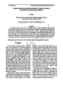
countries i and j. Of the several types of indicators used in the current study, I show examples of how to set up the relevant contiguity matrices for the border-length contiguity and for a minimal-distance contiguity matrix. For this, a simple sample geography is used, with the following shape:

B A

D

E

C

A.1

Border-lenth contiguity

When border-length contiguity is used, the transition matrix, which is the …rst step in creating a contiguity matrix and contains the elements ij , looks as follows: 2 3 2 3 A 0 1 1 0 0 2 7 6 4 7 B 6 1 0 2 1 0 6 7 6 7 7, so row-summing, P = 6 4 7, which makes it possible C 6 1 2 0 1 0 6 7 6 7 4 4 5 D 4 0 1 1 0 2 5 E 0 0 0 2 0 2 to arrive at the actual border-length contiguity matrix,3by dividing the transition 2 0 12 21 0 0 6 1 0 1 1 0 7 6 14 1 2 41 7 7 matrix of the sum of the rows: Wbor = 6 6 4 12 01 4 01 7. 4 0 0 2 5 4 4 0 0 0 1 0 The contiguity matrix now shows the size of the in‡uence of the di¤erent neighbours on the countries. 19

A.2

Minimum-distance contiguity

In the case of minimum-distance contiguity, ij = [(cut + ) (mindistij j mindistij < cut)], where is a pre-determined size, depending on what is practical. In the actual analysis, = 50, but in this example, = 0:5. The distance matrix between all the nations looks as2follows 3 A 0 0 2 3 B 6 0 0 1 7 6 0 7 6 C 6 0 0 0 1 7 7 D 4 2 0 0 0 5 E 3 1 1 0 Taking will look 3 as follows: 2 a cut-o¤ value3of 1:5 and 2 = 3 0:5, the transition 2 matrix A 0 2 2 0 0 4 0 12 21 0 0 7 6 7 6 2 0 2 2 1 7 B 6 6 2 0 2 2 1 7 P 6 7 7 6 72 2 7 27 71 7 7 7 7 6 C 6 =6 6 2 2 0 2 1 7, 6 7 7, so Wmd1:5 = 6 7 71 01 7 17 7 4 5 4 5 4 0 3 3 0 3 5 D 0 2 2 0 2 6 0 14 41 12 0 E 0 1 1 2 0 4 In this case, the weights are obviously di¤erent from the weights found when using the border-length contiguity. Finally, as an example, taking a cut-o¤ value of 2:5 and = 0:5,2the following happens: 2 3 3 3 2 A 0 3 3 1 0 7 0 73 37 17 0 7 6 6 3 0 3 3 2 7 7 B 6 11 11 11 7 6 3 0 3 3 2 7 P 6 11 7 6 11 7, 6 11 7, so Wmd2:5 = 6 3 3 0 3 2 7 C 6 3 3 0 3 2 = 11 11 11 7 6 7 6 6 11 7 4 10 5 4 1 3 3 0 3 5 D 4 1 3 3 0 3 5 10 10 10 10 0 72 27 37 0 E 0 2 2 3 0 7

References [1] Abreu, Maria, Henri L.F. de Groot and Raymond J.G.M. Florax (2004), “Space and Growth”, Tinbergen Institute Discussion Paper, TI 2004-129/3 [2] Ades, Alberto and Hak B. Chua (1997), “Thy Neighbour’s Curse: Regional Instability and Economic Growth”, Journal of Economic Growth, vol. 2, pp. 279-304 [3] Anselin, Luc (1988), Spatial Econometrics, Kluwer Academic Publishers, Dordrecht, the Netherlands [4] Barro, Robert J. and Sala-i-Martin, Xavier (1992), “Convergence”, Journal of Political Economy, vol. 100(2), pp. 223-251 [5] Barro, Robert J. and Jong-Wha Lee (2000), “International Data on Educational Attainment: Updates and Implications”, CID Working Paper, No. 42

20

[6] Baker, Dean (2007), “The Economic Impact of the Iraq War and Higher Military Spending”, CEPR Research Report [7] CIA (2006), The World Factbook, retrieved https://www.cia.gov/cia/publications/factbook/

December

2006,

from

[8] Collier, Paul (1999), “On the Economic Consequences of Civil War”, Oxford Economic Papers, vol. 51, pp. 168-183 [9] Elhorst, J. Paul (2003), “Speci…cation and Estimation of Spatial Panel Data Models”, International Regional Science Review, vol. 26(3), pp. 244-268 [10] Gleditsch, Nils Petter, Peter Wallensteen, Mickael Eriksson, Margareta Sollenberg and Håvard Strand (2002), “Armed Con‡ict 1946-2001: A New Dataset”, Journal of Peace Research, vol. 39(5), pp. 615-637 [11] Gleditsch, Kristian S. and Michael D. Ward (2001), “Measuring Space: A Minimum-Distance Database and Applications to International Studies”, Journal of Peace Research, vol. 38(6), pp. 739-758 [12] Guidolin, Massimo and Eliana La Ferrara (2005), “Diamonds Are Forever, Wars Are Not: Is Con‡ict Bad for Private Firms?”, Federal Reserve Bank of St. Louis Working Paper 2005-004C [13] Harbom, Lotta and Stina Högbladh (2006), UCDP/PRIO Armed Con‡ict Dataset Codebook, Uppsala Con‡ict Data Program (UCDP) and International Peace Research Institute, Oslo (PRIO) [14] Heston, Alan, Robert Summers and Bettina Aten (2006), Penn World Table Version 6.2, Center for International Comparisons of Production, Income and Prices at the University of Pennsylvania [15] Koubi, Vally (2005), “War and Economic Performance”, Journal of Peace Research, vol. 42(1), pp. 67-82 [16] Longo, Roberto and Khalid Sekkat (2001), “Obstacles to Expanding IntraAfrican Trade”, OECD Development Centre Working Paper No. 169 [17] Mankiw, N. Gregory, David Romer and David N. Weil (1992), “A Contribution to the Empirics of Economic Growth”, Quarterly Journal of Economics, vol. 107, pp. 31-77 [18] Miguel, Edward, Shanker Satyanath and Ernest Sergenti (2004), “Economic Shocks and Civil Con‡ict: An Instrumental Variable Approach”, Journal of Political Economy, vol. 112, pp. 725-753

21

[19] Murdoch, James C. and Todd Sandler (2002a), “Economic Growth, Civil Wars and Spatial Spillovers”, Journal of Con‡ict Resolution, vol. 46(1), pp. 91-110 [20] Murdoch, James C. and Todd Sandler (2002b), “Civil Wars and Economic Growth: A Regional Comparison”, Defence and Peace Economics, vol. 13(6), pp. 451-464 [21] Murdoch, James C. and Todd Sandler (2004), “Civil Wars and Economic Growth: Spatial Dispersion”, American Journal of Political Science, vol. 48(1), pp. 138-151 [22] Organski, A.F.K. and Jacek Kugler (1980), The War Ledger, University of Chicago Press [23] Sambanis, Nicholas (2002), “A Review of Recent Advances and Future Directions in the Quantitative Literature on Civil War”, Defence and Peace Economics, vol. 13(3), pp. 215-243 [24] Solow, Robert M. (1956), “A Contribution to the Theory of Economic Growth”, Quarterly Journal of Economics, vol. 25, pp. 65-94 [25] United Nations (2007) http://unstats.un.org

UNStats,

retrieved

March

2007,

from

[26] Worldbank (2007), World Development Indicators, retrieved February 2007, from http://go.worldbank.org/B53SONGPA0

22

Table 1: Baseline short-run regressions, using the violent con‡ict type 1 bench constant 0.171 (0.302) ln(inv) 0.057*** (0.019) ln(sch) 0.031** (0.013) ln(n + g + ) 0.120 (0.096) ln(y0) -0.010 (0.017) conf

confyears 0.169 (0.301) 0.057*** (0.019) 0.031** (0.013) 0.117 (0.095) -0.010 (0.017)

-0.033 (0.081)

conf months (x 100) north R2 N

2

0.147 300

0.147 300

3 4 violent con‡ict confdum confyears 0.148 0.220 (0.295) (0.307) 0.053*** 0.051*** (0.018) (0.019) 0.030** 0.039*** (0.026) (0.014) 0.100 0.117 (0.091) (0.094) -0.011 -0.022 (0.017) (0.020) -0.066* (0.038) -0.056 (0.083) 0.088*** (0.030) 0.161 0.162 300 300

5 confdum 0.203 (0.301) 0.045** (0.018) 0.039*** (0.014) 0.097 (0.090) -0.025 (0.020) -0.081** (0.039)

0.102*** (0.030) 0.181 300

Note: For each of these regressions, OLS regressions are used, with period …xed e¤ects and gr as dependent variable. White’s heteroskedasticity-adjusted standard errors are reported between brackets and * indicates signi…cance at the 10% level, while ** and *** indicate signi…cance at 5% and 1% levels respectively.

23

Table 2: Regressions using one type of con‡ict spill-over and varying over con‡ict type, spill-over type and the presence of a north-dummy 1

2

con‡ict type Wconf type constant

3

4

all dist dist 0.213 0.271 (0.309) (0.314) ln(inv) 0.053*** 0.045** (0.018) (0.018) ln(sch) 0.029** 0.038*** (0.013) (0.014) ln(n + g + ) 0.110 0.109 (0.098) (0.097) ln(y0) -0.011 -0.025 (0.017) (0.019) conf -0.035 -0.045** (0.022) (0.021) conf months (x 100) Wconf conf -0.094 -0.092 (0.082) (0.079) Wconf conf months

civil dist dist 0.211 0.264 (0.313) (0.318) 0.053*** 0.046** (0.018) (0.018) 0.031** 0.040*** (0.013) (0.014) 0.112 0.112 (0.099) (0.098) -0.012 -0.025 (0.017) (0.019) -0.043* -0.050** (0.025) (0.025)

-0.088 (0.077)

-0.078 (0.075)

0.096*** (0.029) 0.176 300

0.162 300

0.092*** (0.029) 0.178 300

north R2 N

0.158 300

5

6

violent dist dist 0.172 0.221 (0.300) (0.304) 0.054*** 0.047*** (0.018) (0.018) 0.032** 0.041*** (0.014) (0.014) 0.101 0.098 (0.092) (0.091) -0.012 -0.025 (0.017) (0.019) -0.066* -0.080** (0.039) (0.040)

-0.175* (0.102)

-0.152 (0.098)

0.168 300

0.098*** (0.030) 0.186 300

Note: For each of these regressions, OLS regressions are used, with period …xed e¤ects and gr as dependent variable. White’s heteroskedasticity adjusted standard errors are reported between brackets and * indicates signi…cance at the 10% level, while ** and *** indicate signi…cance at 5% and 1% levels respectively.

24

Table 3: Comparison of the relevant results between those of Murdoch and Sandler (2002b) and the current paper 1 2 con‡ict type M&S(2002b) Wconf type md100 md100 conf -0.084*** (0.031) conf months -0.121* (x 100) (0.071) Wconf conf -0.109** (0.047) Wconf conf months -0.151 (x100) (0.108) R2 0.21 0.18 N 235 235

3

4

civil md100 md100 -0.046* (0.024) -0.071 (0.062) 0.011 (0.040) 0.007 (0.077) 0.158 0.151 300 300

5

6

violent md100 md100 -0.068* (0.039) -0.034 (0.082) 0.035 (0.047) 0.014 (0.108) 0.162 0.147 300 300

Note: For each of these regressions, OLS regressions are used, with gr as dependent variable. White’s heteroskedasticity-adjusted standard errors are reported between brackets and * indicates signi…cance at the 10% level, while ** and *** indicate signi…cance at 5% and 1% levels respectively. The regressions 3-6 use the adopt the same distance (100k km) as Murdoch and Sandler (2002b)

25

Table 4: Short-run regressions, using two types of con‡ict measure and varying spill-over type and the types of con‡ict 1 type Wconf 1 type Wconf 2 type constant ln(inv) ln(sch) ln(n + g + ) ln(y0) conf conf months (x 100) Wconf 1 conf

2 all

dum md250 0.234 (0.302) 0.047*** (0.018) 0.032** (0.014) 0.116 (0.095) -0.022 (0.019) -0.042** (0.020)

dum md250 0.248 (0.304) 0.053*** (0.020) 0.038** (0.015) 0.114 (0.094) -0.028 (0.019)

-0.073 (0.059)

-0.366*** (0.127) Wconf 1 conf months -0.823*** (x 100) (0.296) Wconf 2 conf 0.421*** (0.139) Wconf 2 conf months 0.855*** (x 100) (0.299) north 0.094*** 0.097*** (0.029) (0.029) R2 0.200 0.191 N 300 300

3

4

civil dum dum md250 md250 0.261 0.238 (0.306) (0.306) 0.047*** 0.050** (0.018) (0.020) 0.033** 0.038** (0.014) (0.015) 0.118 0.112 (0.097) (0.094) -0.024 -0.026 (0.019) (0.020) -0.053** (0.023) -0.091 (0.061) -0.335** (0.133) -0.537** (0.264) 0.377*** (0.139) 0.561** (0.269) 0.094*** 0.095*** (0.029) (0.029) 0.195 0.177 300 300

5

6

violent dum bor md250 md250 0.215 0.262 (0.290) (0.308) 0.044** 0.049** (0.018) (0.019) 0.040*** 0.040*** (0.014) (0.014) 0.092 0.120 (0.086) (0.094) -0.031 -0.028 (0.019) (0.020) -0.080** (0.040) -0.060 (0.084) -0.607*** (0.194) -0.542*** (0.187) 0.655*** (0.199) 0.581*** (0.220) 0.112*** 0.099*** (0.028) (0.031) 0.210 0.180 300 300

Note: For each of these regressions, OLS regressions are used, with period …xed e¤ects and gr as dependent variable. White’s heteroskedasticity-adjusted standard errors are reported between brackets and * indicates signi…cance at the 10% level, while ** and *** indicate signi…cance at 5% and 1% levels respectively.

26

Table 5: Robustness checks for the short-run regressions, displaying results with Correlates of War data (columns 1 and 2), without estimated data (3), without extreme observations (4) and without Botswana (5) 1

2

3

CoW dum bor ms300 md450 0.229 0.242 (0.318) (0.315) ln(inv) 0.053*** 0.050*** (0.019) (0.019) ln(sch) 0.042*** 0.040*** (0.014) (0.014) ln(n + g + ) 0.106 0.114 (0.101) (0.097) ln(y0) -0.030 -0.024 (0.184) (0.020) conf -0.030 (0.042) conf months -0.113 (x 100) (0.072) Wconf 1 conf -0.714*** (0.260) Wconf 1 conf months 0.463 (x 100) (0.296) Wconf 2 conf 0.657** (0.269) Wconf 2 conf months -0.798* (x 100) (0.452) north 0.115*** 0.115*** (0.027) (0.033) R2 0.190 0.186 N 300 300 type Wconf 1 type Wconf 2 type constant

dum md250 0.225 (0.364) 0.039* (0.022) 0.032 (0.020) 0.130 (0.113) -0.013 (.025 -0.042 (0.031)

4 all dum md250 -0.053 (0.118) 0.034*** (0.013) 0.027** (0.013) 0.015 (0.032) -0.009 (0.015) -0.032** (0.015)

5 bor md250 0.259 (0.294) 0.039** (0.018) 0.032** (0.014) 0.107 (0.090) -0.027 (0.020) -0.045** (0.020)

-0.227 (0.139)

-0.302*** (0.106)

-0.182** (0.078)

0.299** (0.148)

0.327*** (0.117)

0.224** (0.094)

0.107*** (0.037) 0.220 191

0.087*** (0.025) 0.209 296

0.114*** (0.029) 0.183 292

Note: For each of these regressions, OLS regressions are used, with period …xed e¤ects and gr as dependent variable. White’s heteroskedasticity-adjusted standard errors are reported between brackets and * indicates signi…cance at the 10% level, while ** and *** indicate signi…cance at 5% and 1% levels respectively.

27

Table 6: Long-run regressions for general con‡ict type, varying over con‡ict spill-over type and the presence of a north dummy Wconf 1 type Wconf 2 type constant ln(inv) ln(sch) ln(n + g + ) ln(y0) conf

1 2 md400 md950 -3.008 (3.841) 0.409** (0.151) 0.193* (0.099) -0.575 (1.132) -0.087 (0.123) -0.043 (0.258)

-2.458 (3.844) 0.403** (0.165) 0.081 (0.116) -0.627 (1.336) -0.041 (0.119)

conf months (x 100) Wconf 1 conf

-0.032 (0.058)

Wconf 1 (x 100) Wconf 2 conf

0.177 (0.233)

0.960 (0.695) conf months

Wconf 2 conf months (x 100) north R2 N

0.243 39

0.204 39

3 4 dum dum md250 ms150 -3.890 -2.021 (3.715) (4.361) 0.337** 0.431** (0.143) (0.175) 0.163* 0.055 (0.090) (0.130) -0.775 -0.440 (1.315) (1.507) 0.009 -0.032 (0.132) (0.121) -0.050 (0.224) -0.019 (0.066) -3.566 (2.150) -1.937* (1.024) 4.535* (2.243) 2.006* (1.040)

0.302 39

0.284 39

5 dum ms250 -1.966 (3.692) 0.266* (0.140) 0.237** (0.099) -0.515 (1.326) -0.164 (0.141) -0.182 (0.229)

6 dum ms150 -1.377 (4.459) 0.332* (0.174) 0.122 (0.126) -0.435 (1.550) -0.136 (0.123)

-0.024 (0.059) -4.205 (3.053) -1.905 (1.172) 4.877 (3.003) 1.955 (1.185) 0.734*** 0.649*** (0.219) (0.214) 0.386 0.361 39 39

Note: For each of these regressions, OLS regressions are used, with period …xed e¤ects and gr as dependent variable. White’s heteroskedasticityadjusted standard errors are reported between brackets and * indicates signi…cance at the 10% level, while ** and *** indicate signi…cance at 5% and 1% levels respectively.

28

Table 7: Long-run regressions for civil con‡ict type, varying over con‡ict spillover type and the presence of a north dummy Wconf 1 type Wconf 2 type constant ln(inv) ln(sch) ln(n + g + ) ln(y0) conf

1 dum

2 md950

-2.976 (4.046) 0.415** (0.160) 0.094 (0.099) -0.904 (1.381) -0.039 (0.132) -0.169 (0.285)

-3.908 (4.127) 0.412** (0.169) 0.070 (0.117) -1.057 (1.443) 0.001 (0.119)

conf months (x 100) Wconf 1 conf

-0.017 (0.060)

Wconf 1 (x 100) Wconf 2 conf

0.274 (0.280)

-0.102 (0.572) conf months

Wconf 2 conf months (x 100) north R2 N

0.195 39

0.207 39

3 4 dum dum md200 md400 -3.526 -3.899 (3.803) (4.147) 0.437*** 0.458** (0.153) (0.193) 0.125 0.060 (0.098) (0.121) -0.863 -1.112 (1.344) (1.453) -0.005 -0.027 (0.131) (0.121) -0.058 (0.252) -0.042 (0.062) -4.073 (2.544) -0.668 (0.498) 4.164 (2.525) 0.898 (0.571)

0.247 39

0.263 39

5 dum ms250 -2.214 (3.697) 0.274* (0.140) 0.222** (0.097) -0.655 (1.318) -0.164 (0.142) -0.193 (0.241)

6 dum md250 -1.841 (4.58) 0.342* (0.185) 0.099 (0.124) -0.596 (1.598) -0.121 (0.126)

-0.052 (0.055) -3.991 (2.985) -0.921 (0.815) 4.568 (2.903) 1.009 (0.831) 0.903*** 0.646*** (0.296) (0.209) 0.371 0.330 39 39

Note: For each of these regressions, OLS regressions are used, with period …xed e¤ects and gr as dependent variable. White’s heteroskedasticityadjusted standard errors are reported between brackets and * indicates signi…cance at the 10% level, while ** and *** indicate signi…cance at 5% and 1% levels respectively.

29

Table 8: Long-run regressions for violent con‡ict type, varying over con‡ict spillover type and the presence of a north dummy Wconf 1 type Wconf 2 type constant ln(inv) ln(sch) ln(n + g + ) ln(y0) conf

1 2 md950 md950 -4.515 (4.197) 0.377** (0.162) 0.086 (0.107) -1.293 (1.477) 0.009 (0.112) -0.223 (0.175)

-3.632 (4.144) 0.426** (0.168) 0.071 (0.115) -0.986 (1.432) -0.017 (0.117)

conf months (x 100) Wconf 1 conf

0.007 (0.092)

Wconf 1 (x 100) Wconf 2 conf

0.366 (0.362)

0.584 (0.428) conf months

3 dum md300 -6.723 (4.005) 0.434** (0.162) 0.106 (0.111) -1.963 (1.394) 0.044 (0.111) -0.150 (0.168)

-2.132** (1.028)

-0.027 (0.079)

-3.749*** (0.775)

-3.990*** (0.843) 2.763** (1.301)

3.883*** (0.814)

0.212 39

0.308 39

6 dum ms150 -2.357 (3.732) 0.314* (0.154) 0.179* (0.100) -0.815 (1.288) -0.160 (0.108)

-2.523** (1.179)

2.773** (1.209)

0.244 39

5 dum md250 -4.831 (3.679) 0.304* (0.164) 0.184* (0.105) -1.597 (1.311) -0.084 (0.112) -0.214 (0.178)

-0.061 (0.094)

Wconf 2 conf months (x 100) north R2 N

4 dum ms150 -3.437 (3.781) 0.402** (0.162) 0.091 (0.114) -0.956 (1.296) -0.030 (0.112)

0.346 39

0.753*** (0.259) 0.390 39

4.000*** (0.869) 0.723*** (0.211) 0.440 39

Note: For each of these regressions, OLS regressions are used, with period …xed e¤ects and gr as dependent variable. White’s heteroskedasticity-adjusted standard errors are reported between brackets and * indicates signi…cance at the 10% level, while ** and *** indicate signi…cance at 5% and 1% levels respectively.

30